L型邊界且為非均質非等向水層的半解析解

國 立 交 通 大 學

環 境 工 程 研 究 所

碩 士 論 文

L 型邊界且為非均質非等向水層的半解析解

Transient groundwater flow in heterogeneous and

anisotropic aquifers with L-shaped boundaries

研 究 生：朱 韻 如

指 導 教 授：葉 弘 德 教授

L 型邊界且為非均質非等向水層的半解析解

Transient groundwater flow in heterogeneous and

anisotropic aquifers with L-shaped boundaries

研 究 生：朱韻如

Student：Yun-Ju Chu

指導教授：葉弘德

Advisor：Hund-Der Yeh

國 立 交 通 大 學

環 境 工 程 研 究 所

碩 士 論 文

A Thesis

Submitted to Institute of Environmental Engineering College of Engineering

National Chiao Tung University in Partial Fulfillment of the Requirements

for the Degree of Master of Science in Environmental Engineering June, 2012 Hsinchu, Taiwan

中 華 民 國 一 ○ 一 年 六 月

L 型邊界且為非均質非等向水層的半解析解

研究生：朱韻如

指導教授：葉弘德

國立交通大學環境工程研究所

摘 要

瞭解地下水層的水位空間分佈與水文地質參數，是評估地下水資源的開發量或整治 地下水污染的重要課題。以新竹含水層為案例，此含水層被斷層及河流圍繞，其形狀近 似為L形。本研究係建立數學模型，在定水頭邊界(河流)及不透水邊界(斷層)侷限下的L 形含水層，模擬地下水經多口井抽水後的暫態水力水頭分佈，此模型將考慮含水層的異 質性和非等向性。首先透過區域分割法建立數學模型，將該含水層分割成兩個子區域。 此模式考慮每個子區域各有不同的水力傳導係數，且各區域含水層皆具非等向性。藉由 分離變數法及考慮子區域間水位與流通量的連續條件，推導出Laplace域的半解析解。所 求得的解用來模擬L形含水層在抽水下的暫態水力水頭分佈；若L形含水層受汙染時，此 解可提供地下水流況資料，協助規劃地下水汙染物控制。此半解析解可更進一步描述梯 形含水層經抽水後的洩降分佈，本解亦可作為數值模式的驗核工具，分析數值模式在L 形凹角邊界處計算上可能產生的水位誤差。 關鍵詞：不規則邊界、非等向、沖積扇含水層、水力傳導係數、區域分割法

Transient groundwater flow in heterogeneous and

anisotropic aquifers with L-shaped boundaries

Student：Yun-Ju Chu

Advisor：Hund-Der Yeh

Institute of Environmental Engineering

National Chiao Tung University

ABSTRACT

Understanding groundwater flow distribution is important for evaluating groundwater resource and dealing with groundwater pollution problems. This study considers an aquifer bounded by faults and rivers in Hsinchu, Taiwan, and the aquifer can be approximately to have an L-shaped domain. A mathematical model is developed to describe the transient groundwater flow due to multiple pumping in an anisotropic, heterogeneous aquifer with an L-shaped domain with impermeable boundary and constant-head boundary representing the fault and the river, respectively. Method of domain decomposition is used to handle such an irregular boundary by dividing the aquifer into two sub-regions with different hydraulic conductivities. Taking into account the continuity conditions of hydraulic head and flux at the boundary between two sub-regions, the solution of the model in Laplace domain is then derived by the method of separation of variables. The semi-analytical solution can be used to assess the groundwater resources in transient pumping effect and provide flow information for pump-and-treat design if the aquifer has contamination. The solution can also be applied to delineate the hydraulic head distributions in aquifers with trapezoid boundary and to verify

the numerical solutions which might give inaccurate results at the corner of the irregular boundary.

Keywords: irregular boundary, anisotropy, alluvial aquifer, hydraulic conductivity, method of

誌

謝

首先誠摯的感謝指導教授葉弘德博士，老師悉心的教導使我得以深入探討地下水領 域專業且廣博的知識，每週定期討論並指點我正確的方向，使我在這些年中獲益匪淺。 老師對學問的嚴謹更是我輩學習的典範。其次感謝中央大學葉高次教授、陳瑞昇教授、 萬能科技大學楊紹洋教授於口試中提出之建議與意見，令通篇論文更顯完整。 感謝雅琪、彥如、其珊、珖儀、璟勝、佩蓉、昭志、國豪、裕霖等學長姐，家豪、 佳琪兩位好同窗，以及芷萱、欣慈、翊岷等學弟妹；平日於研究室中的生活點滴、討論 研究、趕作業的革命情感、令人期待的下午茶時光等……使兩年的研究生活像個溫馨的 大家庭。另特別感謝雅琪學姐給予細心的指導、井然有序的解惑，使本論文得以順利完 成，從學姐身上學習邏輯思考與寶貴經驗令我備感珍惜且終身受用。 感謝環工所諸位師長、全體同學，與大家共同參與的修課、活動仍記憶猶新；感謝 一直以來相知相惜的好朋友們，總能在我挫折時給予鼓勵；感謝其翰在背後的支持，總 是不辭辛勞聆聽我訴說研究室的每一天。 最後，謹以此文獻給我摯愛的家人，謝謝父母的教誨以及長期資助，使我成為現在 的自己，在此有說不完的感謝。

TABLE OF CONTENTS

摘要……….. i ABSTRACT………. ii 誌謝……….. iv TABLE OF CONTENTS………. v LIST OF TABLE………... vi

LIST OF FIGURES……….. vii

CHAPTER 1 INTRODUCTION………. 1

CHAPTER 2 MATHEMATICAL MODEL……… 4

2.1 Conceptual Model………..……… 4

2.2 Governing Equation and Related Boundary and Initial Condition ……….. 4

CHAPTER 3 NUMERICAL RESULTS………. 10

3.1 Steady-State Head Distribution………... 10

3.2 Spatial and Temporal Head Distribution... 11

3.3 Effect of Heterogeneity..……….……….….….….…... 11

3.4 Multi-Pumping/Injection Wells... 12

3.5 Trapezoid Aquifer………... 12

CHAPTER 4 CONCLUTIONS….……….. 14

REFERENCES………...……….. 15

APPENDIX A: STEADY STATE SOLUTIONS FOR AN L-SHAPED AQUIFER WITHOUT PUMPING ...…... 18

LIST OF TABLE

Table 1. Notations……….………... 24 Table 2. The constant-head boundaries and the anisotropic ratio of the hydraulic

LIST OF FIGURES

Figure 1. Map of an aquifer in Hsinchu, Taiwan..……..…...……..…..…..…..…………... 26 Figure 2. An L-shaped alluvial aquifer with two sub-regions………... 27 Figure 3. Steady-state hydraulic head distribution in the aquifer with anisotropic ratio of

(a) 1, (b) 2, (c) 0.5………... 28 Figure 4. Hydraulic head distributions in aquifers with Kx =Ky =520 m/day at time

(a) 2 hrs, (b) 2 days, (c) 7 days.………... 29 Figure 5. Transient hydraulic head distributions induce by pumping at t=7 days in (a) heterogeneous aquifer and (b) homogeneous aquifer………... 30 Figure 6. Hydraulic head distributions induced by two injection wells and one pumping

well at t =1 day……… 31 Figure 7. (a) A trapezoid aquifer (b) The head distribution induced by two pumping wells

CHAPTER 1 INTRODUCTION

Groundwater is an important water resource for agricultural, municipal and industrial uses. The planning and management of water resources through investigation of the groundwater flow is one of the major tasks of practicing engineers. The groundwater flow is highly dependent on the type and shape of the boundaries, especially when the aquifer domain has irregular shape. Most literatures dedicated to the development of analytical models for flow in finite aquifers were to investigate the problems with, for example, rectangular boundary [Chan et al., 1976; Chan et al., 1977; Daly and Morel-Seytoux, 1981; Latinopoulos, P., 1982; Corapcioglu et al., 1983; Latinopoulos, P., 1984; Latinopoulos, P., 1985], wedge-shaped boundary [Chan et al., 1978; Falade, 1982; Holzbecher, 2005; Yeh et al., 2006; Yeh et al., 2008; Chen et al., 2009; Sedghi et al., 2009; Sedghi et al., 2010], or triangle boundary [Asadi-Aghbolaghi et al., 2010]. However, it may not be uncommon that the boundaries of finite aquifers are irregular in real world. For irregular aquifer domain with variable boundary conditions, the solutions of the mathematical model are generally developed by numerical approaches such as finite element methods and finite difference methods. Taigbenu [2003] solved the problems for transient flow in multi-aquifer systems with arbitrarily domain geometry based on the Green element method (GEM). Recently, various computer codes based on either finite difference or finite element algorithms, such as AQUIFEM-N, BEMLAP, FEMWATER, FTWORK, MODFLOW, and SUTRA, were adopted to simulate a variety of groundwater flow problems [Loudyi et al., 2007]. When modeling a complex groundwater flow due to pumping/injection in heterogeneous aquifer with irregular domain boundary and various types of boundary conditions, numerical methods are more suitable than analytical models. However, numerical models usually require large amounts of hydrologic information as input data and CPU time for simulating complicated problems.

Besides, some numerical applications are restricted by criteria of spatial and temporal discretization for avoiding stability and/or numerical dispersion problems. Thus, deriving an analytical model for describing the groundwater distribution in an aquifer with irregular domain boundaries is also beneficial from a practical point of view.

Kuo et al. [1994] applied the image well theory and Theis’ equation to predict transient drawdown behavior in an aquifer with irregularly shaped boundaries. However, the number of the image wells should be increased if the aquifer has very irregular and asymmetric boundary because insufficient number of the image wells might result in divergence [Matthews et al., 1954]. Read and Volker [1993] presented analytical solutions for steady seepage through hillsides with arbitrarily flow boundaries. They used the least squares method for estimating the coefficients in a series expansion of the Laplace equation. The least squares estimators, nevertheless, are equivalent to those derived using orthogonal function, that is, the basis function must be orthogonal [Carrier and Pearson, 1991]. Li et al. [1996] generalized and extended the results of Read and Volker [1990; 1993] and Read [1993] for Laplacian porous-media flow problems involving arbitrarily boundary conditions. The solution procedure was obtained by means of an infinite series of orthonomal functions, and they introduced a method, called image-recharge method, to establish the recurrence relationship of the series coefficients. Currently, Patel et al. [2011] used the method of decomposition adopted from Adomian [1994] to develop similarly analytical models for simulating groundwater flow in aquifers with irregular boundaries. The magnitude of hydraulic head was however underestimated and some conditional restrictions are still required.

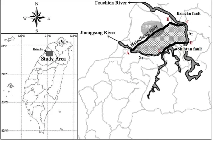
Complication may arise when the boundaries of aquifer domain are irregular. An aquifer in Hsinchu, Taiwan, sketched in Figure 1 is an example. The figure illustrates the plan view of faults and rivers within the aquifer, which may be considered as an L-shaped

aquifer. More detailed description about this aquifer is given in section 2.1. The shading area in this schema designates the study area, which is adjacent to the Hsinchu Science Park (HSP). There are many semiconductor, optoelectronics, and LCD (liquid crystal display) panel factories in the HSP. It was reported that the HSP had the problem of DNAPL (dense non-aqueous phase liquid) contamination in groundwater in the past. The purpose of study is to provide an analytical tool for simulating the flow field if the pump-and-treat method is adopted for pollution remediation. To simplify this problem, the shape of the aquifer within the study area is approximated by a region delineated in Figure 2. This thesis aims at developing an analytical model to describe the groundwater flow in such an aquifer with anisotropic and non-homogeneous hydraulic conductivities. The L-shaped aquifer is divided into two sub-regions that each has a rectangular domain with homogeneous hydraulic conductivity. In addition, two types of boundary conditions, i.e., constant-head boundaries and no-flow boundaries, are used to represent the physical reality and constrain the problem domain. The Laplace-domain solution of the model is obtained after solving the governing equation along with boundary and continuity conditions via the Fourier finite cosine transform and the Laplace transform. A steady-state solution before pumping is first developed to obtain the initial hydraulic head distribution in this L-shaped aquifer. Gaver-Stehfest algorithm is then taken to inverse Laplace-domain solution, and a series of transient hydraulic head distributions in time domain within the problem domain are obtained. These semi-analytical solutions can be used to predict various groundwater flow fields if different pump-and-treat schemes are considered in the remedial design for the L-shaped aquifer.

CHAPTER 2 MATHEMATICAL MODEL

2.1 Conceptual model

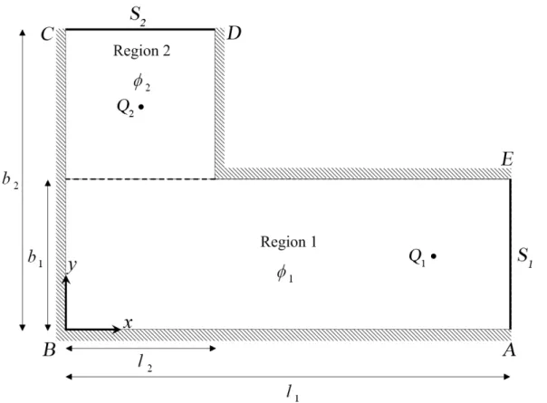
Figure 1 shows a schema for an aquifer in Hsinchu, which is situated in the northwest of Taiwan. The study area is confined by the Hsinchu fault in the north, the Hsincheng fault in the west, the Shihtan fault in the southeast, the Touchien River in the east, and the Jhonggang River in the south. Physically, faults and perennial rivers can be considered as impermeable boundaries and constant-head boundaries, respectively. To simplify this problem, the domain of the study area is approximated to be L-shaped, as delineated in Figure 2. The origin of the coordinate is at the intersection of boundary AB and boundary BC. The Hsincheng fault, the Hsinchu fault, and the Shihtan fault, which are separately represented as boundaries AB, BC, and DE, are considered as impermeable boundaries. The Jhonggang River and the Touchien River, which are respectively expressed as boundaries S and ₁ S , ₂

are considered as constant-head boundaries. This L-shaped aquifer is divided into two sub-regions, named regions 1 and 2 and the hydraulic heads in these two regions are expressed as φ₁=(x,y,t) and φ₂ =(x,y,t).

2.2 Governing equation and related boundary and initial condition

The governing equation describing the hydraulic head distribution in region 1 for the

k th well located at (x_1k,y_1k) with a pumping rate per unit width of Q_1k [L2 /T] is expressed as

∑

= − − − ∂ ∂ = ∂ ∂ + ∂ ∂ M k k k k s y x Q x x y y t S y K x K 1 1 1 1 1 1 2 1 2 1 2 1 2 1 δ( )δ( ) φ φ φ , 1 0≤ x≤l , 0≤ y≤b₁ (1)

and the hydraulic head distribution in region 2 for the kth well located at (x_2k,y_2k) with a pumping rate per unit width of Q_2k [L2/T] is

∑

= − − − ∂ ∂ = ∂ ∂ + ∂ ∂ N k k k k s y x Q x x y y t S y K x K 1 2 2 2 2 2 2 2 2 2 2 2 2 2 δ( )δ( ) φ φ φ , 2 0≤ x≤l , b₁ ≤ y≤b₂ (2) where subscripts 1 and 2 denote the regions 1 and 2, respectively, Ss[ ]

1 −

L is the specific storage, Kx[L/T] and Ky[L/T] are the hydraulic conductivities in x- and y-direction,

respectively. The Dirac delta function δ (⋅) [L−1] is defined in Table 1. The boundary conditions for region 1 can be expressed as:

1 1 =h φ , at x= , l1 0≤ y≤b1 (3) 0 1 = ∂ ∂ x φ , at x=0, 0≤ y≤b₁ (4) 0 1 = ∂ ∂ y φ , at y=0, 0≤x≤l1 (5) 0 1 = ∂ ∂ y φ , at y= , b₁ l₂ ≤ x≤l₁ (6) and the boundary conditions for region 2 are

0 2 = ∂ ∂ x φ , at x=0, b₁ ≤ y≤b₂ (7) 0 2 = ∂ ∂ x φ , at x= , l₂ b₁ ≤ y≤b₂ (8) 2 2 =h φ , at y= , b2 0≤x≤l2 (9)

The continuity requirements of hydraulic head and flux at y= are, respectively, b₁

) , ( ) , ( _{1 2 1} 1 x b φ x b φ = , at 0≤ x≤l₂ (10)

and 1 1 2 2 1 1 b y y b y y y K y K = = ∂ ∂ = ∂ ∂φ φ , at 0≤ x≤l₂ (11)

In order to express the solutions in dimensionless form, following dimensionless variables are introduced: φ₁* =(φ₁−h₁)/h₁ , φ₂* =(φ₂−h₁)/h₂ , t* =K_y1t/S_s1b₂2 ,

1 1 1 =Kx /Ky κ , κ2 =Kx2/Ky2, 1 * / l x x = , 2 * / b y y = , where φ and 1* * 2

φ stand for the dimensionless hydraulic heads for regions 1 and 2, respectively, *

t refers to the dimensionless time during the test, κ and ₁ κ represent the anisotropic ratio of hydraulic ₂ conductivity in region 1 and 2, respectively, x* and y denote the dimensionless coordinate *

variables, b₁* is the dimensionless y-direction distance from the origin to the outer boundary of region 1 (i.e. b₁* =b₁/ b₂), and l is the dimensionless x-direction distance from the origin ₂*

to the outer boundary of region 2 (i.e. l₂* =l₂ / l₁). In addition, Q and _1k* Q are lumped _2k*

parameters defined as b₂2Q_1k　/K_y1h₁ and b₂2Q_2k　/K_y2h₂, respectively.

A steady-state hydraulic head distribution should be obtained as an initial condition for solving the transient flow equation during Laplace transform. Detailed derivation for steady-state solutions for regions 1 and 2 before pumping are given in Appendix A, and the results are, respectively, expressed as

) cos( ) , ( ) , ( * 0 * 1 1 * * * 1 x y C E m y mx m m m λ φ

∑

∞ = ∆ =

(12) and ) cos( )) , ( ) , ( ( ) , ( * 0 * * 2 2 * * * 2 x y D F n y B n y nx n n n α φ

∑

∞ = + ∆ =

(13)

) 1 ( 2 1 2 * 2 0 , *₎ 2 * , ( =∆n − Ω y− n e h h h l y n B

(14) * 1 * 1 ) , (_{m y}* _e my _e my E = Ω + −Ω

(15) ) 2 ( *₎ 2 * 2 * , (_{n y} =_e−Ω ny −_eΩ n y − F

(16)

where the symbols ∆ , 1m ∆ , 2n λ , m α , n Ω , 1m Ω , and 2n ∆n,0 are defined in Table 1. The coefficients in C1m and D2n are solved simultaneously from following two equations

∫

∫

∑

∞ = ∆ ₌ ∆ = ₁ 0 * * 2 0 * * * 0 * * 1 2 1 2 1 2 2 1 ) ( cos ) cos( ) cos( ) , ( ' ) , ( ' * 2 * 1 * x dx dx x x y m E y n F h h K K D C m l n m n y _{y b} y m n n m λ α λ (17) and ) , ( ) , ( ) ( cos ) cos( ) cos( ) , ( ) , ( * 1 * 1 0 * 0 * 2 * 0 * * * 1 * 1 2 1 2 1 1 2 * 2 * 2 b n F b n B dx x dx x x b n F b m E h h C D m l n l n m n m m n − ∆ ∆ =

∑

∫

∫

∞ = α α λ

(18) with * * * ( , ) ) , ( ' y y m E y m E ∂ ∂ =

(19) * * * ( , ) ) , ( ' y y n F y n F ∂ ∂ =

(20)

Since the initial condition is available, the solution of hydraulic head for a heterogeneous, anisotropic aquifer with L-shaped domain can be obtained via finite cosine transform and Laplace transform. The derivations for transient solutions are given in Appendix B and the results of the dimensionless hydraulic heads in Laplace-domain for regions 1 and 2 are, respectively,

) cos( )) , , ( ~ ) , , ( ( ) , , ( ~ * * * 1 * 1 0 1 1 * * * 1 x y p T E i y p p i y p ix i i i φ λ φ =

∑

∞ ∆ + = (21) and ) cos( )) , , ( ) , , ( ( ) , , ( ~ * * 2 * 2 0 2 2 * * * 2 x y p T E j y p F j y p jx j j j α φ =

∑

∞ ∆ + =

(22) with * * ) , , ( * 1 y y _i i _e e p y i E = µ + −µ

(23) ) 2 ( * 2 * * ) , , ( = − jy − j y − e e p y j E θ θ

(24) ) ( )) ( sinh( ) cos( 1 ) , ( 2 1 ) , , ( ~ * 1 * 1 * * 1 * 1 * 1 0 2 1 2 * 1 , 1 * * 1 k M k k i k i k i m i m m i m m p y y H y y x Q p y m E C p y i − − + Ω − Λ ∆ =

∑

∑

= ∞ = µ λ µ µ φ 　　　　　

(25) ) , , ( ~ ) , 1 , ( ~ ) , , ( ( 1) ₂* * 2 1 2 * 2 0 , ) 1 ( * 2 * 2 * * p y j e h h h p l e p j p y j F =−φ _p θj −y +∆_j − θj y− +φ _p

(26) ) ( )) ( sinh( ) cos( 1 ) , ( ) , ( 2 ) ) 1 ( ( ) , , ( ~ * 2 * 1 * * 2 * 2 * 2 * 1 * 2 2 2 2 0 2 1 1 2 * 2 , 2 ) 1 ( 2 1 2 * 2 ) 1 ( 2 * 2 2 1 2 2 1 1 2 , * * 2 * * jj N k k j k j jj j n j n n y y s s j n j y y j y y s s o j p y y H y y x Q p b n F y n F D K K S S l e h h h p l e l h h h K K S S p y j j j − − + Ω − Λ ∆ + − + − − ∆ =

∑

∑

= ∞ = − − θ α θ θ θ φ θ θ 　　　　　 　　　　　

(27)

where p is the Laplace variable and the symbols α , j λ , i µ , i θ , j ∆j,0, ∆1i

,

∆2j

,

Λm,i, j

n,

Λ , and H(⋅) are described in Table 1.

The coefficients in Eqs. (21) and (22) are obtained via continuity conditions of hydraulic head and flux. They can be solved by following two equations simultaneously

* 1 * * 2 * 1 * * 2 * 1 * ) , , ( ' ) , , ( ' ~ ) ( cos ) cos( ) cos( ) , , ( ' ) , , ( ' ) ( cos ) cos( ) cos( ) , , ( ' ) , , ( ' * 1 * * 1 1 0 * * 2 0 * * * 0 * 1 * 2 1 2 1 2 1 2 1 0 * * 2 0 * * * 0 * 1 * 2 1 2 1 2 1 2 2 1 b y p i l j i j y _{y b} y i j i l j i j y _{y b} y i j j i p y i E p y i dx x dx x x p y i E p y j F h h K K dx x dx x x p y i E p y j E h h K K T T = ∞ = ₌ ∞ = ₌ − ∆ ∆ ∆ ∆ =

∫

∫

∑

∫

∫

∑

φ λ α λ λ α λ 　　 　＋　

(28) and ) , , ( ) , , ( ) ( cos ) cos( ) cos( ) , , ( ) , , ( ~ ) ( cos ) cos( ) cos( ) , , ( ) , , ( * 1 2 * 1 2 0 0 * * 2 0 * * * * 1 2 * 1 * 1 2 1 2 1 0 0 * * 2 0 * * * * 1 2 * 1 1 2 1 2 1 1 2 * 2 * 2 * 2 * 2 p b j E p b j F dx x dx x x p b j E p b i h h dx x dx x x p b j E p b i E h h T T i l j l j i p j i i l j l j i j i i j − ∆ ∆ + ∆ ∆ =

∑

∫

∫

∑

∫

∫

∞ = ∞ = α α λ φ α α λ 　　

(29) with * * 1 * 1 ) , , ( ) , , ( ' y p y i E p y i E ∂ ∂ =

(30) * * 2 * 2 ) , , ( ) , , ( ' y p y j E p y j E ∂ ∂ =

(31) * * 2 * 2 ) , , ( ) , , ( ' y p y j F p y j F ∂ ∂ =

(32) * * * 1 * * 1 ) , , ( ~ ) , , ( ' ~ y p y i p y i p p _∂ ∂ = φ φ

(33)

CHAPTER 3 NUMERICAL RESULTS

Following sections present the investigations of the head distribution in the L-shaped aquifer, the effect of anisotropy and heterogeneity of the problem domain, and transient pumping effect with multi-well locations in regard to the aquifer parameters for predicting flow field bounded by constant-head and no-flow boundaries.

3.1. Steady-state head distribution

Consider a hypothetical aquifer with two sub-regions. Region 1 has an area of 900 m

× 300 m while the area of region 2 is 300 m × 300 m. The heads at boundaries x=900 m and y=600 m are respectively kept at h₁=85 m and h₂ =80 m, specific storage is 4

10−

1 −

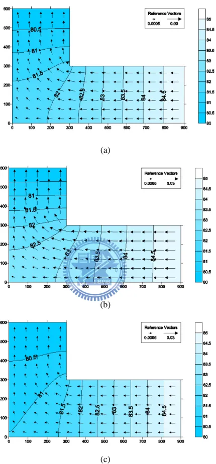
m for those two regions, and the aquifer thickness is 80 m. Figure 3 shows the steady-state hydraulic head distribution, predicted by Eqs. (12) and (13), in the aquifer before pumping. Three different anisotropic ratios of hydraulic conductivity values, 1, 2, and 0.5, are considered in cases (a) - (c) listed in Table 2 and the simulated head distributions are shown in Figures 3a – 3c. The aquifer shown in Figure 3a is isotropic (i.e.,

= = = = _{1 2 2} 1 y x y x K K K

K 520 m/day). This figure displays that the groundwater flows from right to left, because the hydraulic head at boundary x=900 m is higher than that at boundary

=

y 600 m. The flow field schematic diagram is obtained by Darcy’s law with hydraulic head distribution in order to express direction and magnitude of flow velocity. The result illustrates that the flow field in region 1 is mainly in x-direction while that in region 2 is in

y-direction. This is because the shape of the aquifer and the no-flow boundaries constrain

flow paths. The effect of anisotropy on the groundwater flow is demonstrated in Figures 3b and 3c. These three figures indicate that the flow velocity in x-direction increases with anisotropic ratio.

3.2. Spatial and temporal head distribution

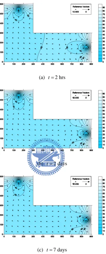
Since the transient solution developed in this study is in Laplace domain, Laplace inversion technique is required to obtain the hydraulic head distributions in real time. Stehfest algorithm [Stefest, 1970; Chang et al., 2010] is used to numerically inverse the transient solution. The hydraulic head distributions at three different times, i.e., t=2 hrs, 2 days, and 7 days are shown in Figures 4a – 4c, respectively. Two wells are installed at (850 m, 150 m) and (150 m, 550 m) with a pumping rate 16 m /3 day and the conductivities

x

K and K_y are 520 m /day for both regions 1 and 2. Those figures show that the

aquifer drawdown increases with pumping time. The differences in hydraulic heads shown in Figures 4b and 4c is very small, indicating that the groundwater flow becomes steady after 2 days pumping in this simulated scenario.

3.3. Effect of heterogeneity

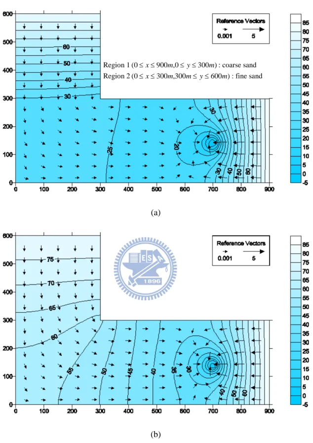
Figure 5 demonstrates the effect of heterogeneity on the groundwater distribution. Two types of aquifer formation materials, coarse sand and fine sand, are considered for the present aquifer system. In Figure 5a, the aquifer in region 1 with coarse sand medium has hydraulic conductivity of 520 m/day while that in region 2 with fine sand medium has hydraulic conductivity of 50 m/day. In contrast to Figure 5a, the aquifer shown in Figure 5b is considered to be homogeneous with coarse sand medium. The well with pumping rate of 8m /3 day is located at (x,y)= (700 m, 140 m). The hydraulic head distribution shown in these two figures are significantly different at t=7 days. The drawdown shown in Figure 5a is much larger than that in Figure 5b because the aquifer in region 2 is relatively low permeable.

3.4. Multi-pumping/injection wells

The effect of the well locations upon the hydraulic head distribution in an aquifer with irregular boundary is investigated in Figure 6. The conductivities K and _x K are 520 _y

m/day for the whole region. One pumping well with a rate of 6m /3 day is located at (100

m, 100 m) and two injection wells with a rate of 3m /3 day are placed at (400 m, 150 m) and

(150 m, 400 m). Figure 6 illustrates that the groundwater flow within the contaminated area can be restrained by those three wells. As demonstrated here, the semi-analytical solution can be used to predict the flow field induced by multi-wells in an L-shaped aquifer. Coupled with an optimization algorithm, this solution can be used to determine the well number, well locations, and their pumping rates for pump-and-treat design in an L-shaped aquifer if it has been contaminated.

3.5. Trapezoid aquifer

The present solutions can also be used to predict the flow induced by pumping in a trapezoid aquifer with 45 degree at the acute angle as shown in Figure 7. Following two conditions must be met if employing the present solution to predict the flow in a trapezoid aquifer. They are the aquifer must be isotropic and homogeneous and the hydraulic heads at two constant-head boundaries have to be equal. A dashed line can be drawn between two re-entrant angles as shown in Figure 7b and an imaginary pumping well should be placed at the location which is symmetric to the pumping well with respect to the dashed line. Thus, the dashed line can be considered as an impermeable boundary for the trapezoid aquifer. Figure 7b demonstrates the transient drawdown distribution at t= 2 days for the pumping well located at (180 m, 76 m) and (76 m, 180 m) with the rate of 40 m /3 day. The

conductivities K and x Ky are

2 10

2× − m /s and specific storage S is s

5 10

1× − m for −1

the whole region, and the hydraulic heads at the boundaries (x= 200 m and y=200 m) are equal to 30 m. The aquifer thickness is 20 m. As a result, a symmetric pattern of the hydraulic head distribution can be observed in the figure. The hydraulic head distribution in the right trapezoid aquifer with a pumping well shown in Figure 7a can therefore be simulated as a part of hydraulic head distribution in Figure 7b. To our knowledge, the semi-analytical solution describing the flow induced by pumping in trapezoid aquifers has never before been presented. The solution derived herein for an L-shaped aquifer can accordingly be applied to solve the flow problems in trapezoid aquifers.

CHAPTER 4 CONCLUDING REMARKS

A new semi-analytical model has been developed to analyze the hydraulic head distributions induce by pumping in a heterogeneous and anisotropic aquifer with an L-shaped domain. Method of domain decomposition is used to divide the aquifer into two sub-regions with different hydraulic conductivities. Steady-state solution is first derived and used as the initial condition before pumping in the L-shaped aquifer system. The Laplace-domain solution of the model is derived using the Fourier finite cosine transform and the Laplace transform. The Stehfest algorithm is then adopted to evaluate the time-domain results. The effects of anisotropy, heterogeneity, and boundary conditions due to pumping are investigated. The present solutions can describe the steady-state and transient distribution of hydraulic head induced by pumping in L-shaped aquifers. Following conclusions can be drawn from this study:

1. The steady-state hydraulic head distributions indicate that the flow in region 1 is mainly in

x-direction and in region 2 is in y-direction.

2. The anisotropic ratio has a significant effect on the flow pattern. The flow velocity in

x-direction increases with anisotropic ratio.

3. The developed solution can be used to assess the effects of heterogeneity and multi-well locations on the head distribution. In addition, it can also be used to solve the flow problems in trapezoid aquifers.

REFERENCES

Adomian, G. (1994), Solving frontier problems in physics – The decomposition method

(fundamental theories of physics), 1 ed., Kluwer Acad. Pub., Dordrecht, The

Netherlands.

Asadi-Aghbolaghi, M., and H. Seyyedian (2010), An analytical solution for groundwater flow to a vertical well in a triangle-shaped aquifer, J. Hydrol., 393(3-4), 341-348.

Carrier, G. F., and C. E. Pearson (1991), Ordinary differential equations, SIAM, Philadelphia, Penn.

Chan, Y. K., N. Mullineux, and J. R. Reed (1976), Analytic solutions for drawdowns in rectangular artesian aquifers, J. Hydrol., 31(1-2), 151-160.

Chan, Y. K., N. Mullineux, and J. R. Reed (1977), Analytic solution for drawdown in an unconfined-confined rectangular aquifer, J. Hydrol., 34(3-4), 287-296.

Chan, Y. K., N. Mullineux, J. R. Reed, and G. G. Wells (1978), Analytic solutions for drawdowns in wedge-shaped artesian aquifers, J. Hydrol., 36(3-4), 233-246. Chang, Y. C., and H. D. Yeh (2010), A new analytical solution solved by triple series

equations method for constant-head tests in confined aquifers, Advances in Water Resources, 33(6), 640-651.

Chen, Y. J., H. D. Yeh, and S. Y. Yang (2009), Analytical solutions for constant-flux and constant-head tests at a finite-diameter well in a wedge-shaped aquifer, Journal of

Hydraulic Engineering, 135(4), 333-337.

Corapcioglu, M. Y., O. Borekci, and A. Haridas (1983), Analytical solutions for rectangular aquifers with 3rd-kind (Cauchy) boundary-conditions, Water Resour. Res., 19(2), 523-528.

Boussinesq groundwater flow equation, Water Resour. Res., 17(4), 875-884. Falade, G. K. (1982), On the flow of fluid in the wedged anisotropic porous domain, J.

Hydrol., 58(1-2), 111-121.

Holzbecher, E. (2005), Analytical solution for two-dimensional groundwater flow in presence of two isopotential lines, Water Resour. Res., 41(12), W12502.

Kuo, M. C. T., W. L. Wang, D. S. Lin, C. C. Lin, and C. J. Chiang (1994), An image-well method for predicting drawdown distribution in aquifers with irregularly shaped boundaries, Ground Water, 32(5), 794-804.

Latinopoulos, P. (1982), Well recharge in idealized rectangular aquifers, Advances in Water

Resources, 5(4), 233-235.

Latinopoulos, P. (1984), Periodic recharge to finite aquifiers from rectangular areas, Advances

in Water Resources, 7(3), 137-140.

Latinopoulos, P. (1985), Analytical solutions for periodic well recharge in rectangular aquifers with 3rd-kind boundary-conditions, J. Hydrol., 77(1-4), 293-306.

Li, P., F. Stagnitti, and U. Das (1996), A new analytical solution for Laplacian porous-media flow with arbitrary boundary shapes and conditions, Mathematical and Computer

Modelling, 24(10), 3-19.

Loudyi, D., R. A. Falconer, and B. Lin (2007), Mathematical development and verification of a non-orthogonal finite volume model for groundwater flow applications, Advances in

Water Resources, 30(1), 29-42.

Matthews, C. S., F. Brons, and P. Hazebroek (1954), A method for determination of average

pressure in bounded reservoir, Trans. AIME, 201, 182-191.

Patel, A., and S. E. Serrano (2011), Decomposition solution of multidimensional groundwater equations, J. Hydrol., 397(3-4), 202-209.

boundary conditions and irregular boundaries, Mathematical and Computer Modelling,

17(12), 9-19.

Read, W., and R. Volker (1990), A computationally efficient solution technique to Laplacian

flow problems with mixed boundary conditions, James Cook University of North

Queensland (Townsville, Q, Australia).

Read, W., and R. Volker (1993), Series solutions for steady seepage through hillsides with arbitrary flow boundaries, Water Resour. Res., 29(8), 2871-2880.

Sedghi, M. M., and N. Samani (2010), Three-dimensional semianalytical solutions of

groundwater flow to a well in fractured wedge-shaped aquifers, J. Hydrol. Eng., 15(12), 974-984.

Sedghi, M. M., N. Samani, and B. Sleep (2009), Three-dimensional semi-analytical solution to groundwater flow in confined and unconfined wedge-shaped aquifers, Advances in

Water Resources, 32(6), 925-935.

Stehfest, H. (1970), Numerical inversion of Laplace transforms, Commun. ACM, 13(1), 47-49.

Taigbenu, A. E. (2003), Green element simulations of multiaquifer flows with a time-dependent Green's function, J. Hydrol., 284(1-4), 131-150.

Yeh, H. D., and Y. C. Chang (2006), New analytical solutions for groundwater flow in wedge-shaped aquifers with various topographic boundary conditions, Advances in

Water Resources, 29(3), 471-480.

Yeh, H. D., Y. C. Chang, and V. A. Mow (2008), Stream depletion rate and volume from groundwater pumping in wedge-shape aquifers, J. Hydrol., 349(3-4), 501-511.

APPENDIX A: STEADY STATE SOLUTIONS FOR AN

L-SHAPED AQUIFER WITHOUT PUMPING

In accordance with the dimensionless variables defined in section 2.2, Eqs. (1) and (2) can be written, respectively, as

∑

= − − − ∂ ∂ = ∂ ∂ + ∂ ∂ M k k k k x x y y Q t y x l b 1 * 1 * * 1 * * 1 * * 1 2 * * 1 2 2 * * 1 2 2 1 2 2 1 δ( )δ( ) φ φ φ κ , 1 0≤ x* ≤ , * 1 * 0≤ y ≤b (A1) and

∑

= − − − ∂ ∂ = ∂ ∂ + ∂ ∂ N k k k k y y s s y y x x Q t K K S S y x l b 1 * 2 * * 2 * * 2 * * 2 2 1 1 2 2 * * 2 2 2 * * 2 2 2 1 2 2 2 δ( )δ( ) φ φ φ κ , * 2 * 0≤x ≤l , b₁*≤ y*≤1 (A2) The dimensionless boundary conditions for region 1 can be expressed as:

0 * 1 = φ , at x* =1, 0≤ y*≤b₁* (A3) 0 * * 1 = ∂ ∂ x φ , at x* =0, 0≤ y*≤b₁* (A4) 0 * * 1 = ∂ ∂ y φ , at y*=0, 0≤ x*≤1 (A5) 0 * * 1 = ∂ ∂ y φ , at y* = , b₁* l₂*≤ x*≤1 (A6) Similarly, the dimensionless boundary conditions for region 2 are

0 * * 2 = ∂ ∂ x φ , at x* =0, b₁* ≤ y* ≤1 (A7) 0 * * 2 = ∂ ∂ x φ , at x* = , l₂* b₁* ≤ y* ≤1 (A8)

1 1 2 * 2 h h h − = φ , at y*=1, 0≤x* ≤l₂* (A9)

The continuity conditions of hydraulic head and flux in dimensionless form are, respectively, ) , ( ) , ( * ₁* _{2 2}* * ₁* * 1 1 x b h x b hφ = φ , at * 2 * 0≤x ≤l (A10) and * 1 * * 1 * * * 2 2 2 * * 1 1 1 b y y b y y y h K y h K = = ∂ ∂ = ∂ ∂φ φ , at * 2 * 0≤x ≤l (A11)

Without the pumping, the steady-state solution for groundwater flow can be solved after removing all the right-hand side terms in Eqs. (A1) and (A2). Multiplying Eq. (A1) by

)

cos(λ_mx* and integrating it from x* =0 to x* =1 in region 1 with boundary conditions Eqs. (A3) and (A4), Eq. (A1) is then transformed to

0 2 * * 1 2 * 1 2 1 = ∂ ∂ − Ω y m φ φ (A12) with

∫

= 1 0 * * * 1 * 1 φ cos(λmx )dx φ where λ_m = m( +1/2)π, m=0,1,2,3....

Similarly, Eq. (A2) can be transformed via multiplying Eq. (A2) by cos(α_nx*) and integrating it from x* =0 to x* = in region 2 with boundary conditions Eqs. (A7) and l₂*

(A8). The result is

0 2 * * 2 2 * 2 2 2 _∂ = ∂ − Ω y n φ φ (A13) with

∫

= 2* 0 * * * 2 * 2 cos( ) l nx dx α φ φ where * 2 / l n n π α = , n=0,1,2,3....

The general solutions of Eqs. (A12) and (A13) are

* 1 * 1 2 1 * * 1 ( , ) y m y m m m _{C e} e C y m = Ω + −Ω φ (A14) and * 2 * 2 2 1 * * 2( , ) y n y n n n _{D e} e D y n = Ω + −Ω φ (A15) where Ω1m =λm κ1b2 l1 and Ω2n =αn κ2b2 l1. The coefficients C1m, C2m, D1n and

n

D2 are unknowns and to be determined. Using boundary conditions Eqs. (A5) and (A9), the following relation can be obtained

m m C C1 = 2 (A16) and n n _{D e} e l h h h D_{n n} 2 _n 2 2 2 * 2 2 1 2 0 , 1 Ω − Ω − ₋ − ∆ = (A17) where    ≠ = = ∆ 0 , 0 0 , 1 0 , n n n .

Substituting Eqs. (A16) and (A17) into Eqs. (A14) and (A15), the inversions of φ and ₁* *

2

φ lead to Eqs. (12) and (13). The Fourier finite cosine inversions for regions 1 and 2 are

∑

∞ = ∆ = 0 * 1 1 * * 1( , ) ( , )cos( ) m m m m y x y m φ λ φ (A18)

∑

∞ = ∆ = 0 * 2 2 * * 2( , ) ( , )cos( ) n n n n y x y n φ α φ (A19) The coefficients of C_1m and D_2n obtained by using the boundary condition Eq. (A6) and the continuity conditions Eqs. (A10) and (A11) are given in Eqs. (17) and (18), respectively.

APPENDIX B: TRANSIENT STATE SOLUTIONS

Multiplying Eq. (A1) by cos(λ_ix*) and integrating it from *=0

x to x* =1 in region 1 with boundary conditions Eqs. (A3) and (A4), Eq. (A1) can be transformed as

∑

= − − ∂ ∂ = ∂ ∂ + Ω − M k k k i k i Q x y y t y 1 * 1 * * 1 * 1 * * 1 2 * * 1 2 * 1 2 1 cos(λ )δ( ) φ φ φ (B1) with

∫

= 1 0 * * * 1 * 1 φ cos(λix )dx φ where λ_i = +(i 1 / 2) /π l₁*, i=0,1,2,3..., and Ω1i =λi κ1b2 l1.

Similarly, Eq. (A2) can be transformed via multiplying Eq. (A2) by cos(α_jx*) and integrating it from x* =0 to 2*

*

l

x = in region 2 with boundary conditions Eqs. (A7) and

(A8). The result is

∑

= − − ∂ ∂ = ∂ ∂ + Ω − N k k k i k s s y y j Q x y y t S S K K y 1 * 2 * * 2 * 2 * * 2 1 2 2 1 2 * * 2 2 * 2 2 2 cos(λ )δ( ) φ φ φ (B2) with

∫

= 2* 0 * * * 2 * 2 cos( ) l jx dx α φ φ where α_j = jπ/ l₂*, j=0,1,2,3..., and Ω_2j =α_j κ₂b₂ l₁.

Then, taking Laplace transforms with respect to t of Eqs. (B1) and (B2) with the initial conditions Eqs. (12) and (13), respectively, results in

∑

∑

= ∞ = − − Λ ∆ − = ∂ ∂ + − M k k k i k m m i m m i y y x Q p y m E C y 1 * 1 * * 1 * 1 0 * 1 , 1 2 * * 1 2 * 1 2 ) ( ) cos( 1 ) , ( 2 1 ~ ~ δ λ φ φ µ 　　　　　　　 (B3) and

∑

∑

= ∞ = − − + Λ ∆ − = ∂ ∂ + − N k k k j k n n j n n s s y y j y y x Q p y n B y n F D S S K K l y 1 * 2 * * 2 * 2 * 0 * 2 , 2 1 2 2 1 * 2 2 * * 2 2 * 2 2 ) ( ) cos( 1 )) , ( ) , ( ( 2 ~ ~ δ α φ φ θ 　　　　　　　 (B4) with

∫

∞ − = 0 * * * * * * ) , , ( ) , , ( ~ dt e t y i p y i φ pt φ

The general solutions of Eqs. (B3) and (B4) can be expressed as

) , , ( ~ ) , , ( ~ * * 1 2 1 * * 1 * * p y i e T e T p y i _i iy _i iy φ _p φ ₌ µ ₊ −µ ₊ (B5) and ) , , ( ~ ) , , ( ~ * * 2 2 1 * * 2 * * p y j e T e T p y j _j jy _j jy φ _p φ θ θ + + = − (B6) The particular solutions φ~₁*_p(i,y*,p) and φ~₂*_p(j,y*,p) presented as Eqs. (25) and (27) are, respectively, from

* * 1 * * 1 * * 1 ( , , ) 2 ) , , ( 2 ) , , ( ~ * * * * dy p y i e e dy p y i e e p y i y i y y i y p i i i i

∫

∫

Γ − Γ = µ −µ −µ µ µ µ φ (B7) and * * 2 * * 2 * * 2 ( , , ) 2 ) , , ( 2 ) , , ( ~ * * * * dy p y j e e dy p y j e e p y j y j y y j y p j j j j

∫

∫

Γ − Γ = − −θ θ θ θ θ θ φ (B8) with

∑

∑

= ∞ = − − Λ ∆ − = Γ M k k k i k m m i m m Q x y y p y m E C p y i 1 * 1 * * 1 * 1 0 * 1 , 1 * 1 cos( ) ( ) 1 ) , ( 2 1 ) , , ( λ δ (B9)

∑

∑

= ∞ = − − + Λ ∆ − = Γ N k k k j k n n j n n s s y y y y x Q p y n B y n F D S S K K l p y j 1 * 2 * * 2 * 2 * 0 * 2 , 2 1 2 2 1 * 2 * 2 ) ( ) cos( 1 )) , ( ) , ( ( 2 ) , , ( δ α 　　　　　　

(B10)

boundary conditions Eqs. (A5) and (A9), the following relations can be obtained i i T T₂ = ₁ (B11) and )) , , ( ~ ( ₂* ₂* 2 1 2 * 2 0 , 2 2 1 j b p h h h p l e e T T _j =− _j −θj + −θj ∆_j − −φ _p (B12) where    ≠ = = ∆ 0 , 0 0 , 1 0 , j j j .

Substituting Eqs. (B11) and (B12) into Eqs. (B5) and (B6), respectively, the inversions of * 1 ~ φ and * 2 ~

φ lead to Eqs. (21) and (22). The Fourier finite cosine inversions for regions 1 and 2 are

∑

∞ = ∆ = 0 * 1 1 * * 1 (, , )cos( ) ~ ) , , ( ~ i i i i y p x p y i φ λ φ (B13)

∑

∞ = ∆ = 0 * 2 2 * * 2 ( , , )cos( ) ~ ) , , ( ~ j j j j y p x p y j φ α φ (B14)

The coefficients of T_1i and T_2j obtained by using the boundary condition Eq. (A6) and the continuity conditions Eqs. (A10) and (A11) are presented as Eqs. (28) and (29), respectively.

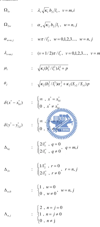
Table 1. Notations. v 1 Ω : λ_v κ₁b₂ l₁, v=m,i w 2 Ω : α_w κ₂ b₂ l₁, w=n, j j n w= , α : wπ/ l₂*, w=0,1,2,3..., w=n, j i m v= , λ : (v+1/2)π/l₁*, v=0,1,2,3..., v=m,i i µ : κ₁(b₂2/l₁2)λ_i2+ p j θ _{: b l S S p} s s j ( / ) ) / ( ₂2 ₁2 2 _{2 2 1} 2 α κ κ + ) ( * 1 * ii x x − δ :     ≠ = ∞ * 1 * * 1 * , 0 , ii ii x x x x ) (y*−y*_2jj δ :     ≠ = ∞ * 2 * * 2 * , 0 , jj jj y y y y q 1 ∆ :     ≠ = 0 , / 2 0 , 2/ * 1 * 1 q l q l , q=m,i r 2 ∆ :     ≠ = 0 , / 2 0 , 1/ * 2 * 2 r l r l , r =n,j 0 , w ∆ :    ≠ = 0 , 0 0 , 1 w w , w=n, j j n, Λ :      ≠ ≠ = = = j , 0 0 , 1 0 , 2 n j n j n

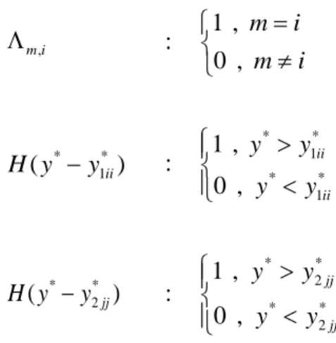
i m, Λ :    ≠ = i m i m , 0 , 1 ) (y* y₁*_ii H − :     < > * 1 * * 1 * , 0 , 1 ii ii y y y y ) ( 2* * jj y y H − :     < > * 2 * * 2 * , 0 , 1 jj jj y y y y

Table 2. The constant-head boundaries and the anisotropic ratio of the hydraulic conductivities for cases (a) – (c)

Case

constant-head

boundary (m) hydraulic conductivity (m/s)

anisotropic ratio of hydraulic conductivity 1 h h₂ Kx1 Ky1 Kx2 Ky2 κ1 a 2 κ a a 85 80 0.003 0.003 0.003 0.003 1 1 b 85 80 0.006 0.003 0.006 0.003 2 2 c 85 80 0.0015 0.003 0.0015 0.003 0.5 0.5 1 κ

a _{represents the anisotropic ratio of the hydraulic conductivity in region 1}

2

κ

Figure 1. Map of an aquifer in Hsinchu, Taiwan. The study area is shaded. (modified from Hydrological year book of Taiwan, 2010, Part II-River stage and discharge, and Taiwan Active Fault Information System)

(a)

(b)

(c)

Figure 3. Steady-state hydraulic head distribution in the aquifer with anisotropic ratio of (a) 1, (b) 2, (c) 0.5.

(a) t=2 hrs

(b) t=2 days

(c) t =7 days

Figure 4. Hydraulic head distributions in aquifers with K_x =K_y = 520 m/day at time (a) 2 hrs, (b) 2 days, (c) 7 days.

(a)

(b)

Figure 5. Transient hydraulic head distributions induce by pumping at t=7 days in (a) heterogeneous aquifer and (b) homogeneous aquifer.

Region 1(0≤x≤900m,0≤ y≤300m): coarse sand Region 2(0≤x≤300m,300m≤ y≤600m): fine sand

Figure 6. Hydraulic head distributions induced by two injection wells and one pumping well at t =1 day.

(a)

(b)

Figure 7. (a) A trapezoid aquifer (b) The head distribution induced by two pumping wells located at (76 m, 180 m) and (180 m, 76 m) at t =2 days.