Predicting the Lifetime of Repairable Unicast
Routing Paths in Vehicle-Formed Mobile Ad Hoc
Networks on Highways
S.Y.
Wang
[email protected]Department
of
Computer Scienceand
InformationEngineering
NationalChiao Tung
UniversityHsinchu,
Taiwan
Abstract-Recently, Intelligent Transportation Systems (ITS) is becoming an important research topic. One goal of ITS is to exchange information between vehicles in a timely and efficient manner. In the ITS research community, inter-vehicle communications (IVC) is considered a way that may be able to achieve this goal.
An information network built on top alf vehicles using IVC can be viewed as a type of mobile ad hoc networks. Although several unicast routing protocols have been proposed for mobile ad hoc networks, how well they can operate on an IVC network is still poorly studied. If generally the lifetime of an established unicast routing path is short on an IVC network, these routing protocols will not perform well for such a network.
Using several vehicle mobility traces generated by a mi- croscopic traffic simulator, this paper anialyzes the lifetime of repairable unicast routing paths existing in an IVC network. Our analytical results can help routing protocols predict the lifetime of a found path. Such a capability can lead to many useful applications.
I. INTRODUCTION
In recent years, Intelligent Transportation Systems (ITS) is becoming popular and an important research topic. ITS aims to providing drivers with safer, more efficient, and more comfortable trips. For example, ITS wants to provide drivers with timely traffic congestion and road condition information
so that drivers can avoid congested or dangerous areas. In ad- dition, ITS wants to provide drivers with1 networking services so that they can exchange information, sendreceive emails, browse web pages from the Internet, etc. To achieve these goals, timely and efficiently distributing and acquiring useful information among vehicles is necessary.
In the ITS research community, inter-vehicle communica- tions (IVC) has attracted the interests of many automobile manufactures and researchers. In such a scheme, no infras- tructure is required for communications between vehicles, and each vehicle is equipped with a wireless radio by which it can send, receive, and forward messages for other vehicles. The vehicles on the roads dynamically form an ad hoc network at any time. Information is distributed, acquired, or exchanged on top of this network. Such an information network can be viewed as a type of mobile ad hoc networks. In the following
of this paper, for brevity, we will simply call such a "vehicle- formed mobile ad hoc network" an IVC network.
Although many studies about mobile ad hoc networks have been done in the past, their results may not be applicable to an IVC network. In such a network, vehicles can move at a high speed such as 120 W h r . In past studies, however, mobile nodes are generally assumed to move at a much lower speed. In addition, vehicles generally move on paved roads with acceleratioddeceleration, lane-changing, and car- following behaviors. However, mobile nodes in past studies are generally assumed to move freely in a random-waypoints fashion, which has recently been found to lead to unreliable results [l]. Due to these differences, the results obtained from past studies about mobile ad hoc networks require re- inspection for their suitability for IVC networks.
In ITS, timely and efficient information distribution, acqui- sition, and exchange among vehicles is important. However, due to the following reasons, it is not easy to achieve these goals. First, an IVC network can easily get partitioned. This situation can easily happen when traffic density is low (e.g., at midnight), when the wireless transmission range is small, when few vehicles are equipped with wireless radios, etc. Second, in an IVC network the data forwarding path (i.e., unicast routing path) between any pair of vehicles can easily break. This situation can easily happen when vehicles are moving in opposite directions. It can also easily happen when vehicles are moving in the same direction but at different speeds because lane-changing now is likely to happen.
This paper studies the lifetime of unicast routing paths in an IVC network, which is built on a simulated highway. We used a commercial microscopic traffic simulator (VISSIM) to generate mobility traces of vehicles moving on the simulated highway. This highway is a closed system (a rectangle) with three lanes in both directions. Its total length is 26 Km. Two thousands vehicles are moving in this system with specified desired speeds. Their acceleratioddeceleration, lane-changing, car-following, and other behaviors are simulated using models well developed in the ITS literature. Using these traces, we derived the lifetime of unicast paths and several other results.
This paper makes two contributions. First, it presents the trends of several performance metrics obtained using reason- able settings and traces. These trends can help researchers gain insights into IVC networks. Second, it presents the absolute performance results of these performance metrics, which are also obtained using reasonable settings and traces. These per- formance results can help routing protocols and higher-layer application programs to make better use of IVC networks. For example, if the predicted lifetime of a found unicast path is too short, it may not be worth using the short-lived path to initiate a long-lived transfer session. As another example, if analytical results show that the lifetimes of unicast paths are mostly short, then routing protocols should be designed to cope with this harsh working condition.
The rest of this paper is organized as follows. Section I1 surveys related work. Section 111 describes the simulation environment and settings. Section IV explains the performance metrics used in this study. In section V, we present the simu- lation results. Finally, we conclude the paper in Section VI.
11. RELATED WORK
In the literature, several papers have discussed and studied the applications of mobile ad hoc networks to IVC networks. In [2], the authors presented the framework and components of their “Fleetnet” project, which aims to efficiently exchanging information among vehicles. In [3], the authors proposed a GPS-based message broadcasting method for inter-vehicle communication. In [4], the authors showed that messages can be delivered more successfully, provided that messages can be stored temporarily at moving vehicles while waiting for opportunities to be forwarded further. In [5], [ 6 ] , the authors
studied how effective a vehicle accident notification message can be distributed to vehicles inside a relevant zone. In [7], the authors focused on how to establish a direct transmission link between two neighboring vehicles.
This paper differs from these existing papers in two ways. First, it uses reasonable mobility traces generated by a mi- croscopic traffic simulator to study IVC-related problems. In contrast, these papers do not use reasonable vehicle mobility traces to study these problems. Second, this paper studies several performance metrics that have not been studied in the past. An example is the lifetime distribution of the unicast routing paths that can be formed among vehicles moving on a highway.
In [8], we studied the effectiveness of distributing informa- tion on an IVC network. The approach taken by that paper is similar to that used in this paper. However, in that paper, we studied broadcast paths while in this paper we focus on unicast paths.
111. SIMULATION SETTINGS A. Trafic Simulator
The microscopic traffic simulator that we used to gen- erate traces of vehicles is VISSIM 3.60 [9], which is a commercial software developed by PTV Planung Transport Verkehr AG company, located in Germany. VISSIM uses the
psycho-physical driver behavior models developed by Wiede- mann [lo], [ 1 11 to model vehicles moving on the highways. This includes acceleratioddeceleration, car-following, lane- changing, and other driver behaviors. Stochastic distributions of speed and spacing thresholds can be set for individual driver behavior. According to the user manual, the models have been calibrated through multiple field measurements at the Technical University of Karlsruhe, Germany. In addition, field measurements are periodically performed to make sure that updates of model parameters reflect recent driver behavior and vehicle improvements.
B. Highways System
The topology of the highway used in this study is depicted in Figure 1. The highway is a rectangular closed system with 3 lanes in each direction. Its length and width are 8 Km and 5 Km, respectively. There are no entrances and exits on this highway system.
Vehicles are injected into this system in both directions at the top-left comer. The injection rate is 1,000 vehicles per hour in each direction. After all vehicles have entered the system, they move freely in the highway system according to their respective desired speeds, vehicles characteristics, and driving behavior.
Since vehicles are assigned different desired speeds and different thresholds for changing lanes for achieving their desired speeds, a vehicle may thus (1) move at its desired speed when there is no slower vehicle ahead of it, (2) follow the lead vehicle patiently, which may happen when the lead vehicle is slower but the difference between the lead vehicle’s speed and its own desired speed is still tolerable, or (3) decide to change lanes to pass the lead vehicle if the speed difference is intolerable.
The vehicle mobility traces are taken after all vehicles have entered the highway system and have been moving for at least one hour. Many traces are taken and each one lasts for 300 seconds. Not that in this highway system, vehicles in different directions do not interact with each other. This is because in this topology a vehicle cannot leave the highway in one direction and then enter the highway in the opposite directions.
C. Vehicle Tra@
In this study, the total number of vehicles moving in the highway system is set to be 2,000 and a half of them are moving in each direction. The average distance between a vehicle and the vehicle immediately following it on the same lane can be calculated. It is (26 Km/lane
*
3 lanes/direction)/ (1,000 vehicles/direction) = 78 meters.The desired speeds chosen for these vehicles determine the absolute speeds of these vehicles and the relative speeds among them. The distribution of these desired speeds is [20%: 100
-
110 M h r , 40%: 90-
100 Km/hr, 20%: 80-
90 Km/hr, 20%: 70-
80 Km/hr], which means that 20% of the vehicles are moving at their desired speeds uniformly distributed between 100 Km/hr and 110 W h r , 40% of the vehicles are are moving at their desired speeds between 90 Kmfhr and 100 Km/hr, etc.I 4
I
b
-
1
Fig. 1. The topology of the highway used in this study. The highway is a rectangular closed system with 3 lanes in each direction. Its length and width
are 8 Km and 5 Km, respectively.
D. W?i-eless Radio
The transmission range of the wireless radios used in these vehicles is chosen to be 100 meters. It is a reasonable setting for the DSRC (Dedicated Short Range Communication) standards proposed for ITS applications.
Since this paper focuses only on the connectivity among vehicles rather than the achievable data transfer throughput among vehicles, this paper does not consider the bandwidth of wireless radios and the medium access control protocol used by them. Instead, we take a simplified approach to determine whether or not two vehicles can success#fully exchange their messages. In our study, as long as two vehicles are within each other’s wireless transmission range, their message exchanges will succeed. Otherwise, their message exchanges will fail. This scheme is similar to that used in the ns-2 simulator [12], except that 250 meters is used as the transmission range of
IEEE 802.11 wireless LAN in ns-2.
IV. STUDIED PERFORMANCES METRICS The studied performance metrics are described in this section. For each metric, we analyze and show its perfor- mances for three different unicast path populations. The first population (SameDIR) consists of all (of the unicast paths whose source and destination vehicles are moving in the same direction in the highway system. The second population (DiffDir) consists of all of the unicast paths whose source and destination vehicles are moving in the opposite directions in the highway system. The third population (BothDir) consists of all unicast paths in the highway system, regardless of the relative moving directions of their source and destination vehicles.
The first performance metric is the lifetime distribution of all of the unicast paths in a particular population. Since most routing protocols such as AODV [ 131 and DSR [ 141 can repair a broken path to resetup a new one, we define the lifetime of a repairable unicast path between two vehicles as the duration
in which there is one path between them. (For brevity, in the following of this paper we will simply use “unicast path” or “path” to represent “repairable unicast path.”) That is, during this period these two vehicles can find a path to exchange their messages, even though this path may need to be changed during this period.
In our study, the path between two vehicles at time T is chosen to be the “shortest” one between them at time T. Note that in our shortest path calculation, we give a wireless link between two vehicles moving in the same direction a distance weight of 1 and a wireless link between two vehicles moving in the opposite directions a distance weight of 10. This is because when setting up a unicast path, we prefer to use those links whose two vehicles are moving in the same direction so
that the found path is less likely to break. Clearly, a wireless link whose two vehicles are moving in the opposite dnections will break very quickly due to their high relative moving speed. The unit of path lifetime is set to be second. Starting from the first second of a trace, in each subsequent second we check whether a unicast path can start. We say that a unicast path between two vehicles starts in N’th second if there exists a path between these two vehicles in N’th second. For each found unicast path, in each subsequent second we then check whether it would end in this second. We say that a unicast path between two vehicles ends in M’th second if there is a path between them in M’th second but no path exists in (M+l)’th second. The lifetime of a unicast path is thus calculated as (M+l)
-
N. Note that, according to the above definition, all unicast paths that can be started in any second during the trace are accounted and processed separately. Also, although in this way each found unicast path has a lifetime of at least 1 second, its exact lifetime actually may be less than 1 second.The lifetime distribution is important as it gives us a sense of how long generally an established unicast path can last on an IVC network. Clearly, we prefer to see long lifetime rather than short lifetime for these unicast paths. Otherwise, many useful unicast-based applications such as email, ftp, http, and telnet are unlikely to be useful on an IVC network.
The second one is the relationship between the lifetimes of unicast paths and their corresponding average hop counts. The hop count of a unicast path between two vehicles is defined to be the number of hops of the path when the path lifetime just begins. Since the hop count of a found routing path can be easily known by routing protocols, this relationship
is
valuable for non GPS-based routing protocols to predict the lifetime of a found routing path on an IVC network. If the predicted lifetime is too short, it may not be worth for them to report a route-search success to the transport layer.The third one is the relationship between the lifetime of unicast paths and their corresponding average physical path length in meters. Like what we did for relating the average hop count of unicast paths to their lifetimes, for each lifetime such as N seconds, we report the average physical length of all unicast paths whose lifetime is N seconds. The physical length of a unicast path between two vehicles is the distance between them when the path lifetime just begins. This relationship is
0 2 -
0
0 5 10 15 20 25 30 35 40 45 50
Unicast Path Lifetime (in seconds)
Fig. 2. IVC network.
The cumulative distribution of the lifetime of unicast paths on an
valuable for GPS-based routing protocols as they can use this information to predict the lifetime of a unicast path.
The fourth one is the relationship between the unicast path lifetime and their corresponding average path length difference (in meters) between the path starting and ending times. Suppose that the path length between two vehicles when the path is initially set up is D1 meters and it becomes D2 meters when the unicast path ends, then the length difference of this path during its lifetime is the absolute value of (D2
-
Dl). This information shows how much a unicast path length can vary during its lifetime and is useful for routing protocols that use dynamic wireless radio power control design. This is because these routing protocols can use this information to set a proper power level to re-reach the destination vehicle.V. SIMULATION RESULTS
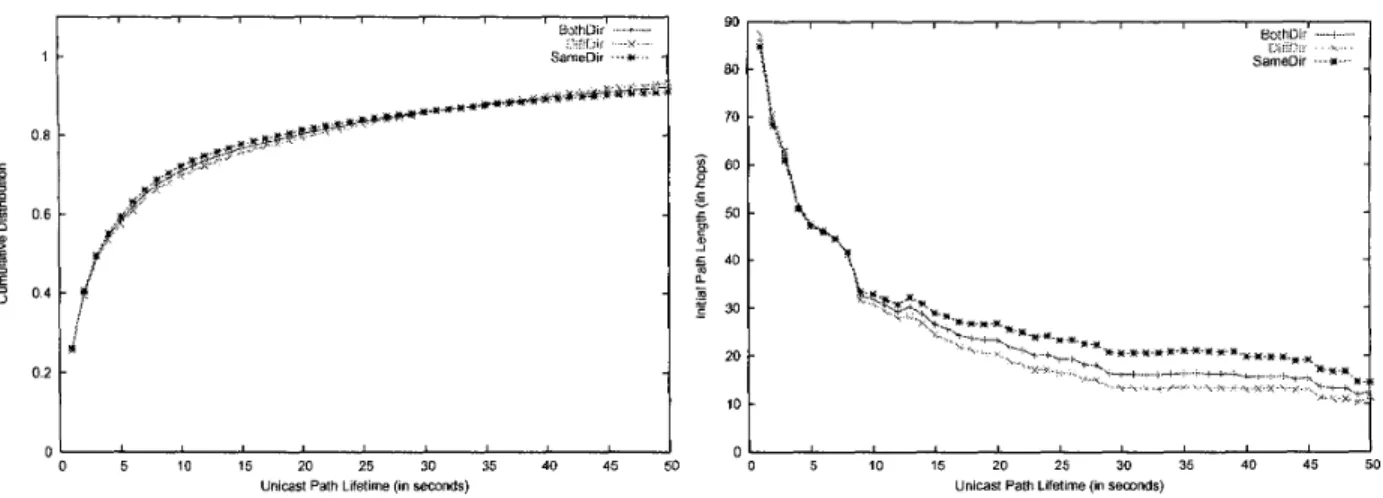
I ) Lifetime Distribution: Figure 2 shows the cumulative distribution of the lifetime of unicast paths found in three different path populations. The Y axis shows the percentage of the unicast paths whose lifetime is less than a particular value. The X axis shows the range between 1 and 50 seconds rather than the whole range between 1 and 300 seconds. This is because for these populations, over 91% of all unicast paths have a lifetime less than 50 seconds. As such, we focus only on this range to see the details.
Surprisingly, the distribution curves of these three different path populations are almost the same. This information lets us know that when a vehicle wants to set up a unicast path to another vehicle, it need not care about whether that vehicle is moving in the same direction with itself. These curves also let us know how long generally a unicast path can last. For example, 70% of all unicast paths have a lifetime less than I O seconds, 80% of all unicast paths have a lifetime less than 20 seconds, etc.
2) Path Hop Number and Lifetime Relationship: Figure 3 shows the relationship between the average hop number of unicast paths and their corresponding lifetime. First, from the
1 l
0 5 10 15 20 25 30 35 40 45 50
Unicast Path Lifetime (in sewnds)
Fig. 3.
IVC network.
The average hop number of unicast paths V.S. their lifetime on an
trend of these curves, we see that as a unicast path needs to traverse more hops to reach its destination vehicle, its lifetime decreases. Second, the absolute performance numbers show that,if a unicast path needs to traverse more than 30 hops, generally its lifetime will be less than 10 seconds. Third, comparing these curves, we see that, beyond 10 seconds and given the same initial path length, a path in the “SameDir” population generally has a longer lifetime than a path in the “DiffDir” population. This phenomenon can be explained as a unicast path whose source and destination vehicles are moving in the same direction will less likely to break than a path whose two vehicles are moving in the opposite directions.
Figure 4 shows the relationship between the average path length of unicast paths (in meters) and their corresponding lifetime. First, from the trend of these curves, we see that as the initial distance between the source and destination vehicles increases, the lifetime of the unicast path between them decreases. Second, if their initial distance is above 2,500 meters, the path lifetime generally is less than 10 seconds. Third, the shape of these curves are almost identical to that in the hop count V.S. lifetime case. For each lifetime, dividing
its initial path length by its corresponding initial hop count gives us a ratio of 77 meterslhop. Amazingly, this ratio of 77 is very close to 78, which is the average distance between a vehicle and the vehicle immediately following it on the same lane (already calculated previously). Fourth, we see that beyond 10 seconds, given the same initial distance, a path in the “SameDir” population generally has a longer lifetime than a path in the “DiffDir” population. The reason for this phenomenon is the same as that discussed above.
4) Path Length Difference between the Path Starting and
Ending nmes: Figure 5 shows the average path length differ- ence (in meters) between the path starting and ending times versus their corresponding lifetime on an IVC network. From these curves, we see that the path length difference generally maintains at a constant and low level for the “SameDir” pop-
5000 4500 4000 p 3500
E
30W 2500 rn-
d .c 2 2000-
2 1500 1000 500 0 Fig. 4.-
te
600 9t
.t
i”5
t1
5 10 15 20 25 30 35 40 45 50UnlcaSt Path Lifetime (In semnds)
The average physical length of unicast paths (in meters) V.S. their lifetime on an IVC network
cot~-n r
-
loo0
7
-
1
0
0 5 10 15 20 25 30 35 40 45 50
Unicast Path Lifetime (in semnds) Fig. 5.
starting and ending times V.S. their lifetime on an IVC network.
The average path length difference (in meters) between the path
ulation. It, however, generally increases with the lifetime for the “DiffDir” population. This phenomenon can be explained as in the “SameDir” case the relative speeid between the source and destination vehicles is very small while in the ‘‘DifDir’’ case it is very large. For this reason, as the lifetime increases, the length difference between the initial and final paths in the “DiffDir” case will be more significant than that in the “SameDir” case.
VI. CONCLUSIONS,
The trends of our results provide insights into IVC networks. In addition, the absolute performance numbers of our results can help routing protocols to predict the lifetime of a found path and thus can better utilize the resource (e.g., bandwidth, battery power, etc.) of an IVC networlk. Such capability is important as now these routing protocols can consider whether it is worth initiating a long-lived transfer on a unicast path whose lifetime is predicted to be short.
In the future, we plan to use the EJCTUns 1.0 network simulator [ 151 to study how real-world protocols would per-
form on IVC networks. The NCTUns 1.0 can take VISSIM’s vehicle mobility trace output as its input and uses real-world TCP/IP protocol stack and applications to generate high- fidelity simulation results. This makes it a suitable tool for studying IVC-related problems.
ACKNOWLEDGMENTS
We would like to thank the anonymous reviewers for their valuable comments. This research was supported in part by MOE Program for promoting Academic Excellence of Univer- sities under the grant number 9 1 -E-FA06-4-4, the Chung-Shan Institute of Science and Technology under the grant number BC93B 13P, and the Ministry of Transportation under the grant number MOTC-STAO-92- 16.
REFERENCES
[I] Jungkeun Yoon, Mingyan Liu, and Brian Noble, ‘Random Waypoint Considered Harmful:’ IEEE INFOCOM 2003, March 2003. [2] Walter J. Franz, Hannes Hartenstein, Brend Bochow, ‘Internet on the
Road via Inter-Vehicle Communications,” Workshop der Informatik 2001: Mobile Communications over Wireless LAN: Research and Appli- cations, Gemeinsame Jahrestagung der GI und OCG, 26-29 September 2001, Wien.
[3] Min-Te Sun, Wu-Chi Feng, Ten-Hwang Lai, Kentaro Yamada, Hiromi Okada, and K i h o Fujimura, ‘GPS-Based Message Broadcasting for Inter-Vehicle Communication:’ 2000 International Conference on Paral-
lel Processing, pp. 279-287.
[4] Zong Da Chen, H.T. Kung, and Dario Vlah, ‘Ad Hoc Relay Wireless Networks over Moving Vehicles on Highways,” The ACM Symposium on Mobile Ad Hoc Networking and Computing (MobiHoc 2001) Poster Paper, October 2001.
[SI Linda Briesemeister, Lorenz Schafers, and Gunter Hormmel, ‘Dissemi- nating Messages among Highly Mobile Hosts based on Inter-Vehicle Communication,” IEEE Intelligent Vehicle Symposium, pp. 522-527, October 2000.
[6] Linda Briesemeister and Gunter Hormmel, ‘Role-based Multicast in Highly Mobile but Sparsely Connected Ad Hoc Networks:’ The First Annual Workshop on Mobile Ad Hoc Networking and Computing (MobiHoc 2000), August 2000.
[7] Tomoyuki Yashiro, Tempei Kondo, Hirotaka Yagome, Masafumi Higuchi, and Yuyuka Matsushita, ‘A Network Based on Inter-Vehicle Communication,” IEEE International Conference on Intelligent Vehicles, pp. 234-250, 1993.
[8] S.Y. Wang, ‘On the Effectiveness of Distributing Information among Vehicles Using Inter-Vehicle Communication”, IEEE ITSC’03 (Interna- tional Conference on Intelligent Transportation Systems), October 12-15, 2003, ShangHai, China.
[9] VISSIM 3.60 User Manual, PTV Planung Transport Verkehr AG com- pany.
[IO] Wiedemann, ‘Simulation des Strabenverkehrsflusses,” Schriftenreihe des Instituts fur Verkehrswesen der Universitat Karlsruhe, Heft 8, 1974. [I 11 Wiedemann, ‘Modeling of RTI-Elements on Multi-Lane Roads,” In:
Advanced Telematics in Road Transport, edited by the Comission of
the European Community, DG XIII, Brussels, 199 1.
[ 121 The Network Simulator - ns-2, available at http://www.isi.edu/nsnam/ns.
[I31 Charles Perkins and Elizabeth Royer, ‘Ad Hoc On Demand Distance Vector Routing,” Second IEEE Workshop on Mobile Computing Sys- tems and Applications, February 1999.
[14] David B. Johoson and David A. Maltz, ‘Dynamic Source Routing in Ad Hoc Wireless Networks,” Mobile Computing, edited by Tomasz Imielinski and Hank Korth, Chapter 5, pp. 153-181, Kluwer Academic Publishers, 1996.
[IS] S.Y. Wang, C.L. Chou, C.H. Huang, C.C. Hwang, Z.M. Yang, C.C. Chiou, C.C. Lin, ‘The Design and Implementation of the NCTUns 1.0 Network Simulator,” Computer Network, Vol. 42, Is- sue 2, pp. 175