具有向量場控制功能的實體材質合成

(1)

國

立

交

通

大

學

多媒體工程研究所

碩

士

論

文

具有向量場控制功能的實體材質合成

Solid Texture Synthesis with Vector Field Control

研究生：蘇雅琳

指導教授：施仁忠教授

張勤振教授

(2)

具有向量場控制功能的實體材質合成

Solid Texture Synthesis with Vector Field Control

研究生：蘇雅琳 Student：Ya-Lin Su

指導教授：施仁忠教授 Advisor：Dr. Zen-Chung Shih

張勤振教授

.Dr.Chin-Chen Chang

國立交通大學

多媒體工程研究所

碩士論文

A Thesis

Submitted to Institute of MultimediaEngineering College of Computer Science

National Chiao Tung University in partial Fulfillment of the Requirements

for the Degree of Master

in

Computer Science

June 2008

Hsinchu, Taiwan, Republic of China

(3)

I

具有向量場控制功能的實體材質合成

Solid Texture Synthesis with Vector Field Control

研究生：蘇雅琳指導教授：施仁忠教授

.

張勤振教授

國立交通大學多媒體工程研究所

摘要

目前對於實體材質合成(solid texture synthesis)的研究，大多以二維切面 (2D slice)來模擬三維合成(3D synthesis)的效果，然而此類方法只記錄立體空間中，三個二維切面(2D slice)上的資料，用做鄰近點比對(neighborhood matching)，對於在立體空間中的其他部份資料則無法拿來利用於材質合成 (texture synthesis)的過程中，使得最後結果會喪失空間中的資料，更甚至無法控制立體空間的材質(texture)方向性。本篇利用立體空間中的鄰近點比對 (neighborhood matching)，發展出一套可以運用在真正三維空間中實體材質合成(solid texture synthesis)的方法；過程中使用表面向量值(appearance vector) 取代傳統只用色彩值 (RGB color value) 來做鄰近點比對 (neighborhood matching)，有了資料量豐富的表面向量值(appearance vector)，我們就可以只比對 8 個點來建立 5×5×5 個點的立方體(cube)內的鄰近點(neighborhood)資料，並且利用額外的向量場(vector field)來達到控制材質方向性(texture control)的目的。

(4)

II

Solid Texture Synthesis with Vector Field Control

Student：Ya-Lin Su Advisor：Dr. Zen-Chung Shih

.Dr. Chin-Chen Chang

Institute of Multimedia Engineering

National Chiao Tung University

ABASTRACT

Recently, some researches have been focusing on solid texture synthesis and most of them use three orthogonal 2D slices to synthesize solid textures. However, these methods only use the information on three 2D slices for neighborhood matching, and the information within 3D space is not used. It makes the results lost some information, and it is unable to control solid textures in the 3D space. Our method presents a new technique for generating solid textures with cube neighborhood matching. It helps us to synthesize within real 3D space. Appearance vectors are used to replace color neighborhood values. With these information-rich vectors, we can only use 8 locations acts for 5×5×5 cube structure neighborhoods. Additionally, we introduce our approach for controllable texture synthesis with vector fields for coherent anisometric synthesis.

(5)

III

Acknowledgements

First of all, I would like to thank my advisors, Dr. Zen-Chung Shih and .Dr. Chin-Chen Chang, for their supervision and helps in this work. Then I want to thank all the numbers in Computer Graphics & Virtual Reality Lab for their comments and instructions. Especially the leader in this Lab, Yu-Ting Tsai, I want to thank him for his suggestions. Finally, special thanks for my family, and this achievement of this work dedicated to them.

(6)

IV

Abstract (in Chinese) ………I Abstract (in English) ...………..II Acknowledgements………...….III Contents………..IV List of Figures………..V CHAPTER 1 INTRODUCTION...………...1 1.1 Motivation...………...1 1.2 Overview...……….3 1.3 Thesis Organization...……….5

CHAPTER 2 RELATED WORKS...………...6

2.1 Texture Synthesis with Control Mechanism...……….6

2.2 Solid Texture Synthesis...………8

CHAPTER 3 SOLID SYNTHESIS PROCESS...………...9

3.1 Feature Vector Generation...………...9

3.2 Similarity Set Generation………..12

3.3 Pyramid Solid Texture Synthesis...………14

3.3.1 Pyramid Upsampling...……….14

3.3.2 Jitter Method...………..15

3.3.3 Voxel Correction...………15

CHAPTER 4 ANISOMETRIC SYNTHESIS PROCESS...………20

4.1 3D Vector Field...………..20

4.2 Anisometric Solid Texture Synthesis...……….23

4.2.1 Pyramid Upsampling...……….23

4.2.2 Voxel Correction...………23

CHAPTER 5 IMPLEMENTATION AND RESULTS...………...28

5.1 Isometric Results.………..29

5.2 Anisometric Results...………..……….39

CHAPTER 6 CONCLUSIONS AND FUTURE WORKS...………57

(7)

List of Figures

Figure 1.1: System flow chart………4

Figure 3.1: Overview of volume data transformation………..11

Figure 3.2: Process for feature vector generation……….12

Figure 3.3: Synthesis from one voxel to m×m×m solid texture………..14

Figure 3.4: Eight neighbors for N_sl( p)………..16

Figure 3.5: Four sub-neighbors for every neighbor of voxel p ………17

Figure 3.6: Process for inferring candidates for voxel p ………...18

Figure 4.1: 5×5×5 3D vector field with orthogonal axes……….21

Figure 4.2: 5×5×5 3D vector field with a circle pattern on XY plane………..22

Figure 4.3: Eight warped neighbors for N~_sl(p)………..25

Figure 4.4: Four warped sub-neighbors for warped neighbors of voxel p …………26

Figure 4.5: Process for inferring warped candidates for voxel p ………..27

Figure 5.1: Input and result data for case_1……….32

Figure 5.8: 5×5×5 3D vector field about circular control………39

Figure 5.9: Anisometric result with circular control for case_5………...40

Figure 5.10: Input data and anisometric result with circular control for case_8……..41

Figure 5.11: 5×5×5 3D vector field about oval control………42

Figure 5.12: Anisometric result with oval control for case_5………..43

Figure 5.13: Anisometric result with oval control for case_8………..44

Figure 5.14: 5×5×5 3D vector field about slant control………...45

Figure 5.15: Input data and anisometric result with slant control for case_9………..46

Figure 5.16: Anisometric result with slant control for case_5……….47 V

(8)

VI

Figure 5.17: 5×5×5 3D vector field about zigzag control………49

Figure 5.18: Anisometric result with zigzag control for case_9………...50

Figure 5.19: Anisometric result with zigzag control for case_5………...…51

Figure 5.20: Anisometric result with zigzag control for case_8………...52

Figure 5.21: 5×5×5 3D vector field about 3D slant control……….53

Figure 5.22: Anisometric result with 3D slant control for case_9………54

Figure 5.23: Anisometric result with 3D slant control for case_5………55

(9)

Chapter 1 Introduction

1.1 Motivation

Recently, a wide range of textures can be synthesized in 2D; even structural

textures such as wood and marble can be synthesized well. But there is still a lack

of techniques in generating 3D textures. There are many different kinds of

techniques for 3D surface texturing, such as texture mapping [7, 20, 21],

procedural texturing [4, 14] and image-based surface texturing [17, 18, 19].

Texture mapping is the easiest way for 3D surface texturing. However, it suffers

the well-know problems of distortion, discontinuity, and unwanted seams.

Procedural texturing can generate high quality 3D surface textures without

distortion and discontinuity, but still some problems exist. First, procedural

texturing models only limit types of textures, such as marble. Second, there are

(10)

on the designers.

Image-based surface texturing can synthesize a wider range of textures, but

it fails for large structural textures such as bricks. And it still suffers the distortion

problem when the curvature is too large. As a result, when 2D textures are used

in texturing 3D objects, there are some disadvantages such as discontinuous

problems, distortion problems on large-curvature surfaces, and non-reusable

problems. Thus, textures generated for one surface can not be used for other

surfaces.

Solid textures can be used to overcome the above problems. Peachey [13]

and Perlin [14] introduced the idea of 3D solid textures considered as a block of

colored points in 3D space to represent a real-world material. Solid textures

obviate the need for finding a parameterization for the surface of the object to be

textured, avoiding the problems of distortion and discontinuity. Moreover, solid

textures provide texture information not only on surfaces, but also inside the

entire volume.

Recently, some methods [3, 10, 15] used three orthogonal slices for

neighborhood matching, but there are some drawbacks within these methods:

They do not include the neighborhood information in 3D space, and they are

(11)

texture synthesis and use vector fields for controllable texture synthesis. The

whole process is totally automatic. We use information-rich appearance vectors

and cube neighborhoods for neighborhood matching. The results show that our

proposed approach can model a wide range of textures.

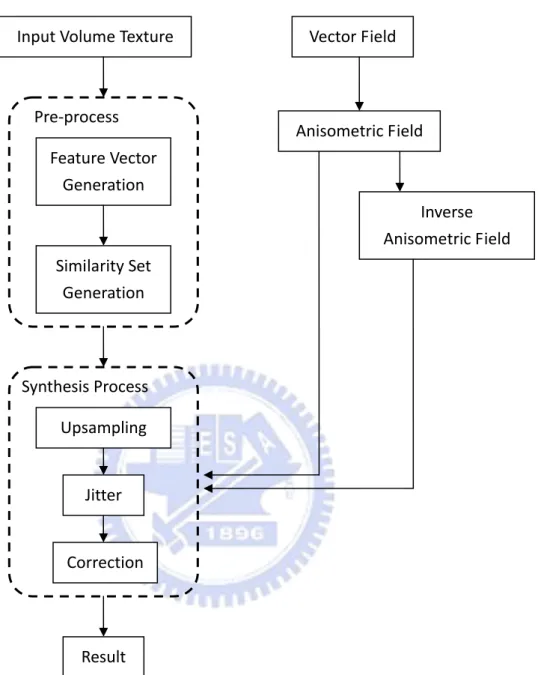
1.2 Overview

The flow of our proposed system is shown in Figure 1.1. First, input a

volume texture data. Then, in the pre-process, feature vectors and similarity sets

are generated. For feature vector generation, it captures 5x5x5 cube information

and applies PCA to reduce the dimension as the voxel RGB color values. For the

similarity set generation, it will find three most similar voxels for each voxel. In

the synthesis process, we apply the pyramid synthesis method in [11] to our

system. Upsampling, jitter and correction are used at each level to get the result.

Furthermore, for the anisomeric synthesis, we use vector fields to control the

results. First, input a vector field as the anisometric field and compute the

inverse anisomertic field from the vector field. When the correction technique is

(12)

Input Volume Texture Feature Vector Generation Anisometric Field Inverse Anisometric Field Similarity Set Generation Pre‐process Upsampling Jitter Synthesis Process Correction Result Vector Field

Figure 1.1 System flow chart

The major contributions of this thesis are as follows: First, we present an

approach for synthesizing solid textures from volume textures. With appearance

vectors, only 8 locations are used to synthesize solid textures, whereas prior

(13)

anisometric synthesis algorithm for solid textures based on vector field control.

1.3 Thesis Organization

The rest of this thesis is organized as follows: In Chapter 2, we review

related works about texture synthesis with control and solid texture synthesis. In

Chapter 3, we present the proposed approach for synthesizing solid textures

from volume textures. Chapter 4 presents the proposed anisometric synthesis

approach for solid textures based on vector field control. The implementation

and results are given in Chapter 5. Finally, conclusions and future works are

(14)

Chapter 2 Related Works

In this chapter, we review previous researches related to our work. We focus on two parts: texture synthesis with control mechanism and solid texture synthesis.

2.1 Texture Synthesis with Control Mechanism

We first review approaches with 2D texture control and 3D surface control.

Ashikhmin [1] presented an algorithm for users to use an interactive painting-style interface to control over the texture synthesis process. He proposed a shift-neighborhood method to find some candidate pixels for neighborhood matching and then searched a best similar neighborhood from them. This approach uses a smaller neighborhood to obtain the quality characteristics of a larger neighborhood and maintains the coherence of the results. Users can control where the patterns appear in the result images. This method provides users an interactive way to control the texture results, and it is fast and straightforward for the users. However, it could not obtain good results if the user’s control does not

(15)

contain significant amount of high frequency components.

Lefebvre and Hoppe [11] introduced a high-quality pyramid synthesis algorithm to achieve parallelism. Their method includes a coordinates upsampling step to maintain patch coherence, jittering of exemplar coordinates to make the texture various, and an order-independent correction approach to improve texture quality. The results would be high-quality and efficient because of the order-independent correction step, it corrects the pixel coordinates after jittering for more accurate neighborhood matching, and the process can be divided into many subpasses to increase efficiency. Only a drawback exists: it will perform poorly if the features are too large to be captured by small neighborhoods. It is also a well known problem for other neighborhood-based per-pixel synthesis methods.

Lefebvre and Hoppe [12] presented a framework for exemplar-based texture synthesis with anisometric control. They used appearance vectors to replace traditional RGB color values for neighborhood matching. Their appearance space makes the synthesis more efficiently because it reduces runtime neighborhood vectors from 5×5 grids to only 4 locations, and produces high-quality results because of the information-rich appearance vectors. They also combined their pyramid synthesis with this method to accelerate neighborhood matching and introduce novel techniques for coherent anisometric synthesis which reproduces arbitrary affine deformations on textures. They provided a convenient method for texture control.

Kwatra et al. [8] presented a method for flow control on 2D textures and they presented an algorithm to achieve texture control on 3D surfaces [9]. They

(16)

provided a novel vector advection technique with global texture synthesis to achieve dynamically changing fluid surfaces. The user-defined fluid velocity fields are used to control the texture results on 3D surfaces, and the neighborhood construction step in the process will consider orientation coherent with it. This approach keeps the synthesized texture similar to the input texture and maintains temporally coherent. The limitation is that it is difficult for the users to define an orientation velocity field which is smooth everywhere.

2.2 Solid Texture Synthesis

Now we review different methods for solid texture synthesis.

Jagnow et al. [6] gave a stereological technique for solid textures. This approach used traditional stereological methods to synthesize 3D solid textures from 2D images. They synthesized solid textures for spherical particles and then extended the technique to apply to particles of arbitrary shapes. Their approach needs cross-section images to record the distribution of circle sizes on 2D slices and builds the relationship of 2D profile density and 3D particle density. Users could use the particle density to reconstruct the volume data by adding one particle at a time, and it means the step is manual. This method uses many 2D profiles to construct 3D density for volume result. Their results are good for marble textures, but their system is not automatic and only for particle textures. Chiou and Yang [2] improved this method to automatic process, but it still only for particle textures.

(17)

gray-level aura matrices (BGLAMs) framework. They used BGLAMs rather than traditional gray-level histograms for neighborhood matching. They created aura matrix from input exemplars and then generated a solid texture from multiple view directions. For every voxel in the volume result, they will only consider the pixels on the three orthogonal slices for neighborhood matching.Their system is fully automatic and requires no user interaction in the process. Furthermore, they can generate faithful results of both stochastic and structural textures. But they needed large storages for large matrix and their results are not good for color textures. They used the information on three slices to create the aura matrix, so they could not do texture control on the results in 3D space.

Kopf et al. [10] introduced a solid texture synthesis method from 2D exemplars. They extended 2D texture optimization techniques to synthesize 3D solid textures and then used optimization approach with histogram matching to preserve global statistical properties. They only considered the neighborhood coherence in three orthogonal slices for one voxel, and iteratively increase the similarity between the solid textures and the exemplar. Their approach could generate good results for wide range of textures. However, they synthesized the texture with the information on the slices. It is difficult to control in 3D space.

Takayama et. al. [16] presented a method for filling a model with anisotropic textures. They had some volume textures and then specify it how to map to 3D objects. They pasted solid texture exemplars repeatedly on the 3D object. Users can design volumetric tensor fields over the mesh, and the texture patches are placed according to these fields.

(18)

Chapter 3 Solid Synthesis Process

In this section, we will present our approach for synthesizing solid textures from volume textures. In Section 3.1, we describe the feature vector in appearance space and how we obtain the feature vectors. Then we use the similarity set to accelerate neighborhood matching in Section 3.2. In Section 3.3, we introduce how to apply 2D pyramid texture synthesis to solid texture synthesis. The upsampling process is to increase the texture sizes between different levels, that every one voxel in parent level will generate eight voxels in children level. The jitter step is to perturb the textures to achieve deterministic randomness. The last step in pyramid solid synthesis is voexl correction, using neighborhood matching to make the results more similar to the exemplar.

3.1 Feature Vector Generation

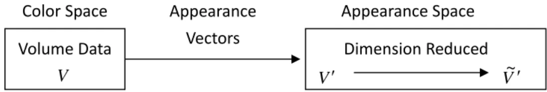
Solid texture synthesis using RGB color values for neighborhood matching needs larger neighborhood size and numerous data. Appearance vectors have been proved that they are continuous and low-dimensional than RGB color values for neighborhood matching. Therefore, we decide to transform the volume data values in color space into feature vectors in appearance space. As shown in

(19)

Fig. 3.1, we transform volume data into appearance space volume data . We use the information-rich feature vectors for every voxel to obtain high-quality and efficient solid texture results.

V V ′

Color Space Appearance Appearance Space

Dimension Reduced V ′ V~ ′ Volume Data Vectors

V

Figure 3.1 Overview of volume data transformation

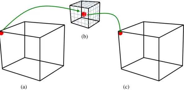
Lefebvre and Hoppe [12] introduced appearance vectors in 2D space, and we will apply it in 3D space. After getting the RGB color values of input volume data, we take the values in 5×5×5 grids (Fig. 3.2 (b)) to construct feature vectors for every voxel in the input volume exemplar (Fig. 3.2 (a)). The exemplar is consisted of the feature vectors at every voxel. There are 375 dimensions (125 for grids and 3 for RGB) for one voxel in

V

V ′

′, and then we perform PCA to reduce the dimensions for a transformed exemplar (Fig. 3.2 (c)). It means that we project the exemplar using PCA to obtain the transformed exemplar .

V~ ′

V ′ V~ ′

We suppose that the data on each side is connected with them on the opposite side. For the voxels on the border, we will treat the voxels on the opposite border as its neighbors, and then take their RGB values to construct feature vectors. However, the data is always not continuous at the borders for some input exemplars. In order to avoid border effect problems, we will discard the data of 2 voxels (about half of 5) on each border, and we compute the feature vectors for the (n−2)×(n−2)×(n−2) voxels in the exemplar V .

(20)

Figure 3.2 The process for feature vector generation

(a) input volume data V (b) 5×5×5 grids structure for feature vectors (c) transformed exemplar V~ ′

3.2 Similarity Set Generation

By the -coherence search method [21], we could find the most similar candidates in the exemplar V for the pixel

k k

p , and then search from the

candidates for neighborhood matching. The method can accelerate neighborhood matching because we do not have to search from each pixel in the exemplar for neighborhood matching. Therefore, we have to construct a similarity set to record the candidates similar to each voxel.

V

k

We apply the 2D -coherence search method [21] to 3D space. In the 3D space, we find the most similar voxels from all voxels in the transformed exemplar for voxel

k k

V~ ′ p , and then construct the candidate set to

record the candidates similar to every voxel

) ( ...

1 p

Cl _K

k p , where l is the pyramid level,

(b)

(c) (a)

(21)

p p C₁l( )=

n n×

, and k is a user-defined parameter.

By the principle of coherence synthesis [1], searching candidates from the neighbors of pixel p in the exemplar V can accelerate the synthesis process. Following this principle, we can find the most similar voxels from the neighbors of voxel

k n

n

n× × p in the transformed exemplar V~ ′ to

construct the similarity set C₁l_..._K(p) for voxel p , where is a user-defined parameter to control the window size for coherent synthesis. In the experiments,

is set as 7.

n

However, it will suffer the local minimum problem if we follow the principle of coherence synthesis [1] because we only consider the

neighbors of voxel

n n n× × p to be candidate voxels for p . We do not consider the

global optimization. Therefore, we reform the method for the similarity set. We still find the k most similar voxels for voxel p in the transformed exemplar V~ ′. In order to avoid the local minimum problem, after finding C , we restrict that the voxel in the

) ( 1 p l n n

n× × neighbors of can not be , and we search from the other voxels besides the

) ( 1 p l n C n ) ( 2 p Cl n× × neighbors of to be . By the same way, the voxel in the

) ( 1 p Cl ) ( 2 p Cl n×n×n neighbors of

can not be C for

) ( p C_nl ) ( 1 p l

n+ p until we construct . Now we finish the

similarity set for the transformed exemplar V

) p ( ... l K 1 C

~ ′, and then we will use the similarity set in synthesis process.

(22)

3.3 Pyramid Solid Texture Synthesis

3.3.1 Pyramid Upsampling

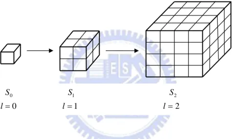
The pyramid synthesis method [5] synthesizes textures from coarse level to fine level. There are levels in synthesis process, l=0~ , where m is the size of the target texture. They synthesized an image from , where . We will apply this 2D pyramid synthesis method to 3D space.

1 + l log2m S S ~₀ S_L m L=log₂ 0 S S₁ S₂ 0 = l l =1 l=2

Figure 3.3 Synthesis from one voxel to m×m×m solid texture

We will synthesize from one voxel to a m×m×m solid texture, from , as shown in Fig. 3.3. We synthesize a volume data in which each voxel stores the coordinate value of the exemplar voxel. At the first, we build a voxel and assign value (1,1,1) to it as coordinate value, and then we upsample the coordinate values of parent voxels for next level, assigning each eight children the scaled parent coordinates plus child-dependent offset.

L S S ~₀

[ ]

p S S

(23)

Δ + = Δ + l₋ l l p S p h S[2 ] ₁[ ] (1) ) (log₂ 2 m l l h = −

{

}

⎟ ⎟ ⎟ ⎠ ⎞ ⎜ ⎜ ⎜ ⎝ ⎛ ⎟ ⎟ ⎟ ⎠ ⎞ ⎜ ⎜ ⎜ ⎝ ⎛ ⎟ ⎟ ⎟ ⎠ ⎞ ⎜ ⎜ ⎜ ⎝ ⎛ ⎟ ⎟ ⎟ ⎠ ⎞ ⎜ ⎜ ⎜ ⎝ ⎛ ⎟ ⎟ ⎟ ⎠ ⎞ ⎜ ⎜ ⎜ ⎝ ⎛ ⎟ ⎟ ⎟ ⎠ ⎞ ⎜ ⎜ ⎜ ⎝ ⎛ ⎟ ⎟ ⎟ ⎠ ⎞ ⎜ ⎜ ⎜ ⎝ ⎛ ⎟ ⎟ ⎟ ⎠ ⎞ ⎜ ⎜ ⎜ ⎝ ⎛ ∈ Δ 1 1 1 , 1 1 0 , 1 0 1 , 1 0 0 , 0 1 1 , 0 1 0 , 0 0 1 , 0 0 0

where denotes the regular output spacing of exemplar coordinates, and means the relative locations for 8 children.

l

h Δ

3.3.2 Jitter Method

After upsampling the coordinate values, we have to jitter our texture to achieve deterministic randomness. We plus the upsampled coordinates at each level a jitter function value to perturb it. The jitter function is produced by a hash function ) ( p J_l

[

]

2 2 1 , 1 : ) (p Ζ → − +

H and a user-defined parameter rl.

) ( ] [ ] [p S p J p S_l = _l + _l (2) l l l p hH p r J ( )= ( )

3.3.3 Voxel Correction

In order to make the coordinates similar to those in the exemplar , we will take the jittered results to recreate neighbors. There is a feature value for every voxel after constructing feature vectors. For every voxel

V

p , we collect the

feature values of its neighbors to obtain the neighborhood vector , and then search the most similar voxel from the transformed exemplar

) p ( N_sl

V~ ′ to make the result similar to the exemplar V .

(24)

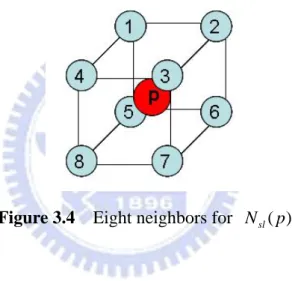
In neighborhood matching, we take 8 diagonal locations for voxel p to obtain the neighborhood vector N_sl( p):

⎪ ⎭ ⎪ ⎬ ⎫ ⎪ ⎩ ⎪ ⎨ ⎧ ⎟ ⎟ ⎟ ⎠ ⎞ ⎜ ⎜ ⎜ ⎝ ⎛ ± ± ± = Δ Δ + = 1 1 1 ]] [ [ ~ ) (p V' S p Nsl (3)

Fig. 3.4 shows the 8 diagonal locations for every voxel p .

Figure 3.4 Eight neighbors for N_sl( p)

By [12], they averaged the pixels nearby pixel p+Δ to improve convergence without increasing the size of the neighborhood vector . They averaged the appearance values from 3 synthesized pixels nearby

as the new feature value at pixel

) ( p N_sl Δ + p Δ +

p , and then used the new feature values at 4 diagonal pixel to construct neighborhood vector N_sl( p).

We apply this approach to perform 3D coordinate correction. First, we average the feature values from 4 synthesized voxels nearby neighborhood voxel of p , p+Δ, as the new feature value at voxelp+Δ. means the averaged feature value at voxel

) ; (p Δ N_sl Δ +

(25)

synthesized voxels for every neighbor. Then we use the new feature values from 8 diagonal voxels to construct neighborhood vectorsN_sl( p).

] ] [ [ ~ 4 1 ) ; ( ' , p+Δ+Δ −Δ′ ⎜ ⎜ ⎜ ⎝ ⎛ ⎟ ⎟ ⎟ ⎠ ⎞ 0 0 0 , 0 0 0 ′ = Δ

∑

_Δ′₌ _Δ _∈_ΨV S p N_sl _M _M (4)

{

}

⎟ ⎟ ⎟ ⎠ ⎞ ⎜ ⎜ ⎜ ⎝ ⎛ ⎟ ⎟ ⎟ ⎠ ⎞ ⎜ ⎜ ⎜ ⎝ ⎛ ⎟ ⎟ ⎟ ⎠ ⎞ ⎜ ⎜ ⎜ ⎝ ⎛ ∈ Ψ 1 0 0 0 0 0 0 0 1 0 0 0 , 0 0 0 0 0 0 0 0 1 , 0 0 0 0 0 0 0 0 0

Figure 3.5 Four sub-neighbors for every neighbor of voxel p

We search the voxel u which is most similar to voxel p by comparing neighborhood vectors and . We use the similarity sets and coherence synthesis method in the searching process, utilizing the 8 voxels nearby voxel

) ( p

N_sl N_sl(u)

p to infer where the voxel u is. For example, for the voxel

neighbor voxel ( ), we can get the most similar 3 voxels ( , , ) for voxel from the similarity set, and then use the relationship between voxel and voxel

i i=1~8 i₁ i₂ i₃

i i

(26)

shown in Fig. 3.6. We set the 3 voxels (i₁_p,i₂_p,i₃_p) as the candidates for voxel p . We compute the neighborhood vectors by the averaged feature values from

the 8 nearby voxels of 3 candiates. We can obtain , , and

. ) (_{1 p} sl i N N_sl(i_{2 p}) ) (i_{3 p} sl N

Figure 3.6 Process for inferring candidates for voxel p . Using three similar voxels of neighbor voxel to infer candidates for voxel i p

In the same way, there are 8 voxel neighbors near voxel p , and each of them has 3 similar voxels. Therefore, we will infer 24 candidates for voxel p . Then we compute the 24 s, where is a candidate, compare these

s with for neighborhood matching, and find the most similar ) (u N_sl u ) (u N_sl N_sl( p) i1 i3 i2 i1p i3p i2p

(27)

voxel u to replace voxel p .

We can synthesize any size for results if the information in the exemplar is enough. It means the size of the input data must be large enough.

(28)

Chapter 4 Anisometric Synthesis Process

In this section, we present the proposed anisometric synthesis approach for solid textures with vector field control. In Section 4.1, we introduce 3D vector fields for texture control and how we generate anisometric fields and inverse anisometric fields with the 3D vector fields. Then we introduce the differences between solid synthesis and anisometric synthesis in Section 4.2. These differences are about upsampling and voxel correction. The jitter step is the same as it in the solid synthesis process.

4.1 3D Vector Field

We need the user-defined 3D vector fields to implement anisometric solid texture synthesis. We use the vector fields to control the result.

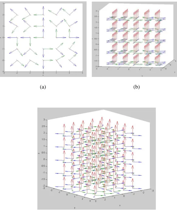
We design a 3D space that contains three orthogonal axes at every point first, and then use mathematics formulas to control the three axes. Fig. 4.1 shows the 3D vector field with orthogonal axes at every point, and the space size is 5×5×5. We make the three axes various, and expect that the texture results would be changed with the fields. For example, we design a circular field, and there will be

(29)

a circular pattern on the texture. Fig. 4.2 shows the 3D vector field with a circular pattern on XY plane. The vector field should be the same size as the texture result.

(a) (b)

(c)

Figure 4.1 5×5×5 3D vector field with orthogonal axes (a) XY plane (b) XZ plane

(30)

(a) (b)

(c)

Figure 4.2 5×5×5 3D vector field with a circle pattern on XY plane (a) XY plane (b) and (c) are three axes at every point

We have to make the anisometric field and the inverse anisometric field for each level with the user-defined 3D vector field,. The anisometric field

A

1 − A

A is made by downsampling the 3D vector field, and we will obtain for

each level. Then, we inverse the to get inverse anisometric field for

l A 1 − l A l A

(31)

each level. In the anisometrc synthesis process, the steps for upsampling and correction will refer to the fields A_l and at each level.

] S 1 − l A ]

4.2 Anisometric Solid Texture Synthesis

4.2.1 Pyramid Upsampling

The goal for upsmapling step in anisometric synthesis is the same as it in isometric synthesis. It helps synthesize from coarse level to fine level, and we have to upsample the coordinate values of parent voxels for the next level.

The difference is that the child-dependent offset for upsmapling step in anisometric synthesis is dependent on the anisometric field . We use the anisometric field to compute the distance for spacing.

A A ) ( [ [p ₁ p h A p S_l = _l₋ −Δ + _lΔ⋅ _l (5) ) l l h =₂(log2m− ⎜ ⎜ ⎜ ⎝ ⎛ ⎟ ⎟ ⎟ ⎠ ⎞ , 5 . 0 5 5

{

}

⎟ ⎟ ⎟ ⎠ ⎞ ⎜ ⎜ ⎜ ⎝ ⎛ ⎟ ⎟ ⎟ ⎠ ⎞ ⎜ ⎜ ⎜ ⎝ ⎛− ⎟ ⎟ ⎟ ⎠ ⎞ ⎜ ⎜ ⎜ ⎝ ⎛ − ⎟ ⎟ ⎟ ⎠ ⎞ − − ⎜ ⎜ ⎜ ⎝ ⎛ − ⎟ ⎟ ⎟ ⎠ ⎞ ⎜ ⎜ ⎜ ⎝ ⎛ − − ⎟ ⎟ ⎟ ⎠ ⎞ ⎜ ⎜ ⎜ ⎝ ⎛ − − ⎟ ⎟ ⎟ ⎠ ⎞ ⎜ ⎜ ⎜ ⎝ ⎛ − − − ∈ Δ 5 . 0 5 . 0 5 . 0 , 5 . 0 5 . 0 5 . 0 , 5 . 0 5 . 0 5 . 0 , 5 . 0 5 . 0 5 . 0 . 0 . 0 , 0 , 5 . 0 5 . 0 5 . 0 , 5 . 0 5 . 0 5 . 0 5 . 0 5 . 5 . 0

where denotes the regular output spacing of exemplar coordinates, and means the relative locations for 8 children.

l

h Δ

4.2.2 Voxel Correction

The goal for correction step is to make the coordinates similar to those in the exemplar V . For every voxel p , we collect the feature values of warped

(32)

neighbors by the anisometric field and the inverse anisometric field to obtain , and then search the most similar voxel from the transformed exemplar l A Al−1 ) ( p N_sl

V~ ′ to make the result similar to the exemplar according to the 3D vector field.

V

The method presented by Lefebvre and Hoppe [12] for anisometric synthesis is able to reproduce arbitrary affine deformations, including shears and non-uniform scales. They only accessed immediate neighbors of pixel p to construct the neighborhood vector . They used the Jacobian field and the inverse Jacobian field to infer which pixel neighbors to access, and the results will be transformed by the inverse Jacobian field at the current point. We will apply this to 3D space.

) p ( N_sl J 1 − J 1 − J

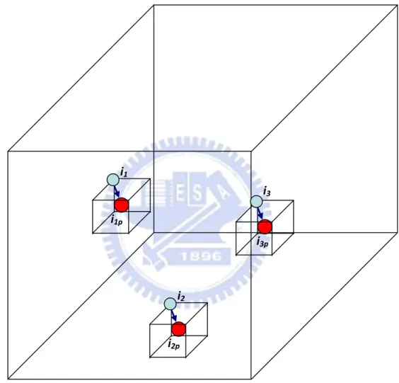
First, we have to know which 8 voxel neighbors to voxel p . We use the inverse anisometric field A_l−1 to infer the 8 warped neighbors for voxel p , and

construct the warped neighborhood vector N~_sl(p):

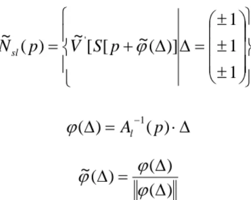
⎪ ⎩ ⎪ ⎨ ⎧ ⎜ ⎜ ⎜ ⎝ ⎛ ± ± ± = Δ Δ + = [ ~( )] ) ( ~ _ϕ p V p Nsl [ ~' S Δ) ( ⎪ ⎭ ⎪ ⎬ ⎫ ⎟ ⎟ ⎟ ⎠ ⎞ 1 1 1 (6) Δ ⋅ = − ) ( 1 p A_l ϕ ) ( ) ( ) ( ~ Δ Δ = ϕ Δ ϕ ϕ

where )ϕ~ Δ( keeps its rotation but removes any scaling.

(33)

are changed from diagonal locations by the inverse anisometric fieldAl−1.

Figure 4.3 Eight warped neighbors for N~sl(p)

Second, we have to find the 4 synthesized voxels nearby warped neoghborhod voxels of voxel p . We use the inverse anisometric field to infer the 4 synthesized voxels for voxel

1 − A ) ( ~ Δ +ϕ p ) (

, and compute the averaged feature value as the new feature value at p+ϕ~ Δ . Fig. 4.4 shows the locations of 4 warped synthesized voxels for each warped neighbor.

] Δ M

{

}

)] ( ~ ) ( ~ [ [ ~ 4 1 ) ; ( ~ ' ), ( ~ ) ( ~ + Δ + ′ Δ − = Δ

∑

′_Δ ₌ _Δ _∈_ΨV S p p N_sl _ϕ _ϕ _M _M ϕ ϕ (7) ⎟ ⎟ ⎟ ⎠ ⎞ ⎜ ⎜ ⎜ ⎝ ⎛ ⎟ ⎟ ⎟ ⎠ ⎞ ⎜ ⎜ ⎜ ⎝ ⎛ ⎟ ⎟ ⎟ ⎠ ⎞ ⎜ ⎜ ⎜ ⎝ ⎛ ⎟ ⎟ ⎟ ⎠ ⎞ ⎜ ⎜ ⎜ ⎝ ⎛ ∈ Ψ 1 0 0 0 0 0 0 0 0 , 0 0 0 0 1 0 0 0 0 , 0 0 0 0 0 0 0 0 1 , 0 0 0 0 0 0 0 0 0

(34)

Figure 4.4 Four warped sub-neighbors for warped neighbors of voxel p

We search the voxel u′ which is most similar to voxel p by comparing neighborhood vectorsN~_sl(p) and N~_sl(u′). We utilize the 8 warped voxels nearby voxel p and the anisometric fields to infer where the voxel is. For example, the warped neighbor voxel

A u′

i′ ( ′i=1~8), we can get the most similar 3 voxels ( , , ) for voxel i′₁ i′₂ i′₃ i′ from the similarity set, and then use the warped relationship with the anisometric fields A between voxel i′ and voxel

p to infer the candidate voxels (i₁′ ,_p i₂′ ,_p i₃′ ) for voxel p , as shown in Fig. 4.5. _p With the candidates for voxel p , we can compute the warped neighborhood vectors )N~_sl(i₁′ ,_p N~_sl(i_{2 p}′ ) and N~_sl(i′_{2 p}) with the inverse anisometric fieldA_l−1.

(35)

3 i′

Figure 4.5 Process for inferring warped candidates for voxel p . Using three

similar voxels of warped neighbor voxel i′ to infer candidates for voxel p

By the same way, we will infer 24 candidates for voxel p , and compute the 24 N~_sl(u′)s, where u′ is a candidate. Comparing these N~_sl(u′)s with N~_sl(p)

for neighborhood matching, we could find the most similar voxel to replace voxel u′ p . 1 i′ i’3p 2 i′ i’1p i’2p

(36)

Chapter 5 Implementation and Results

We implement our system on a PC with 2.67GHz and 2.66GHz Core2 Quad CPU and 4.0GB of system memory. We use MATLAB to implement our method. For a 32×32×32 volume data V , it needs about 3 minutes to construct a transformed exemplar from feature vectors and about 2 hours to construct a similarity set. For a 64×64×64 volume data , it needs about 90~120 minutes for a transformed exemplar

V ′

V

V ′ and about 85~95 hours for a similarity set. The transformed exemplar V from feature vectors and the similarity set can be reused for synthesis process. It means that once the feature vectors and similarity sets are constructed, we can use them for other syntheses with different target sizes for results and with different vector fields.

′

For a 64×64×64 result data, it needs about 6 hours to synthesize solid texture. For a 128×128×128 result data, it needs about 7~10 hours for synthesis process. We will show our results with 64×64×64 input volume data and 128×128×128 result data in this chapter. The detail computation time for different textures are shown in Table 5.1. In Section 5.1, we show some isometric synthesis results, and we show anisometric results with different vector fields

(37)

control in Section 5.2.

We use 5×5×5 grids for feature vectors at each voxel, 7×7×7 grids for similarity set that the voxels in this area could not be the candidate of the center voxel, and the parameter for jitter step is set to 0.7.

5.1 Isometric Results

The input data in Fig. 5.1(b) (case_1) is stochastic and marble-like texture. It only contains two kinds of colors, and it is vivid. It is information-rich that only needs small amount of data to represent the whole texture. It means that we can synthesize larger results (bigger than two times of input data size) with this kind of textures. Fig. 5.1(c)~(f) show the result. As we can see, the result is continuous and not the duplication of the input data.

The input data in Fig. 5.2(b) (case_2) is particle-like texture. It contains few kinds of color, and it is very different between particles and background. The particles in case_2 are the same kind. As long as there are few complete particle patterns in the input data, we can synthesize good result, as shown in Fig. 5.2(c)~(f). Because the few particle patterns can represent whole texture, we can synthesize it from 32×32×32 to 128×128×128, even from 64×64×64 to 256×256×256 volume data (the result size is four times of input size).

The input data in Fig. 5.3(b) (case_3) is another type of particle texture. It contains different sizes and different colors of particles, and most of particles look like the same color as background. Fig. 5.3(c)~(f) show the result from

(38)

64×64×64 to 128×128×128 volume result. Because the input data is not information-rich, the distribution of the particles in the result is sparse, not as it in the input data. It means that the size of the input data is not enough to contain enough information for us to synthesize.

The input data in Fig. 5.4(b) (case_4) is about sea water. It is a kind of homogeneous textures because it is almost in the same color in the whole volume.

The main feature in the input data is the highlight area. As the result in Fig. 5.4(c)~(f) shown, there are few highlight area in the result volume data.

The input data in Fig. 5.5(b) (case_5) is a kind of structural textures. The patterns in the input data are small and compact, so the texture is information-rich. Only small size for input data could contain enough patterns for synthesis. It can be synthesized with a few input data and obtain good results. The result is shown in Fig. 5.5(c)~(f).

The input data in Fig. 5.6(b) (case_6) is structural and continuous on two directions and broken on the other direction. It is consist of thin stokes from black and white. The result in Fig. 5.6(c)~(f) is good at the two continuous directions, which is continuous and not duplicate, but broken at the other direction because the input data is information-poor.

The input data in Fig. 5.7(b) (case_7) is structural with bigger patterns. The feature in the input data is too large, so the input data could not represent the whole volume data if the input size is too small. As we can see in Fig. 5.7(c)~(f), the information in the 64×64×64 input data is regular, not various, so the result is

(39)

not as we expect.

Table 5.1 computation time for different textures

Feature Vector

Construction

Similarity Set Construction

Synthesis Process

Case_1 47.8 seconds 85 hours 37 minutes 7 hours 55 minutes Case_2 31.1 seconds 85 hours 28 minutes 8 hours 17 minutes Case_3 35.4 seconds 86 hours 5 minutes 8 hours 22 minutes Case_4 48.6 seconds 84 hours 42 minutes 8 hours 5 minutes Csse_5 34.3 seconds 83 hours 46 minutes 7 hours 28 minutes Csse_6 38.2 seconds 86 hours 21 minutes 8 hours 41 minutes Csse_7 35.7 seconds 86 hours 51 minutes 8 hours 43 minutes Csse_8 37.3 seconds 93 hours 30 minutes 6 hours 52 minutes Csse_9 34.9 seconds 85 hours 4 minutes 8 hours 43 minutes

(40)

(a) (b)

(c) (d)

(e) (f)

Figure 5.1 Input and result data for case_1

(a) cross sections at X=32, Y=32, and Z=32 for input data

(b) input volume data for case_1

(c) cross section at X=126, Y=126, and Z=126 for result data (d) cross section at X=80, Y=80, and Z=80 for result data (e) cross section at X=64, Y=64, and Z=64 for result data (f) result volume data for case_1

(41)

(a) (b) (c) (d) (e) (f)

(42)

(a) (b) \ (c) (d) (e) (f)

(43)

(a) (b) (c) (d) (e) (f)

(44)

(a) (b) (c) (d) (e) (f)

(45)

(a) (b) (c) (d)

(e) (f)

(46)

(a) (b) (c) (d) (e) (f)

(47)

5.2 Anisometric Results

We show anisometric results with different vector field controls : circular pattern on XY plane, oval pattern on XY plane, slant pattern on XY plane, zigzag pattern on XY plane, and slant control on 3D space. In order to emphasize the control effect, we show the results about structural textures, as brickwalls and woods et. al.

The vector field about circular control is in Fig. 5.8. The results with circular pattern control on the XY plane are shown in Fig. 5.9 and Fig. 5.10. Fig. 5.9 shows the result for case_5. The result is good because of its small and compact pattern. The input data in Fig. 5.10(b) (case_8) is wood texture, it is continuous on the two directions and broken on the other direction. We can see the patterns changed with circular control on XY plane.

(a) (b)

Figure 5.8 5×5×5 3D vector field about circular control

(48)

(a) (b)

(c) (d)

Figure 5.9 Anisometric result with circular control for case_5

(a) cross section at X=126, Y=126, and Z=126 for result data (b) cross section at X=80, Y=80, and Z=80 for result data (c) cross section at X=64, Y=64, and Z=64 for result data (d) anisometric result with circular control for case_5

(49)

(a) (b) (c) (d) (e) (f)

Figure 5.10 Input data and anisometric result with circular control for case_8

(c) cross section at X=126, Y=126, and Z=126 for result data (d) cross section at X=80, Y=80, and Z=80 for result data (e) cross section at X=64, Y=64, and Z=64 for result data (f) anisometric result with circular control for case_8

(50)

The vector field about oval control is in Fig. 5.11. The results with oval pattern control on the XY plane are shown in Fig. 5.12 and Fig. 5.13. Fig. 5.12 shows the result for case_5, it is good at this kind of control. Fig. 5.13 is the result for case_8, it is continuous with the oval control.

(a) (b)

Figure 5.11 5×5×5 3D vector field about oval control

(51)

(a) (b)

(c) (d)

Figure 5.12 Anisometric result with oval control for case_5

(a) cross section at X=126, Y=126, and Z=126 for result data (b) cross section at X=80, Y=80, and Z=80 for result data (c) cross section at X=64, Y=64, and Z=64 for result data (d) anisometric result with oval control for case_5

(52)

(a) (b)

(c) (d)

Figure 5.13 Anisometric result with oval control for case_8

(a) cross section at X=126, Y=126, and Z=126 for result data (b) cross section at X=80, Y=80, and Z=80 for result data (c) cross section at X=64, Y=64, and Z=64 for result data (d) anisometric result with oval control for case_8

(53)

The vector field about slant control is in Fig. 5.14. The results with slant control on the XY plane are shown in Fig. 5.15 and Fig. 5.16. As we can see, there are slant control on XY direction, and no change from isometric results on XZ and YZ direction. The input data in Fig. 5.15(b) (case_9) is about brickwalls, a kind of structural texture. The result in Fig. 5.15(c)~(f) is continuous with the slant control at the whole volume. It is good at the cross sections of different planes. Fig 5.16 shows the result for case_5, there is a little discontinuity on XY plane and no change on the other planes.

(a) (b)

(c) (d)

Figure 5.14 5×5×5 3D vector field about slant control

(a) one axes on XY plane (b) one axes at every point

(54)

(a) (b) (c) (d) (e) (f)

Figure 5.15 Input data and anisometric result with slant control for case_9

(c) cross section at X=126, Y=126, and Z=126 for result data (d) cross section at X=80, Y=80, and Z=80 for result data (e) cross section at X=64, Y=64, and Z=64 for result data (f) anisometric result with slant control for case_9

(55)

(a) (b)

(c) (d)

Figure 5.16 Anisometric result with slant control for case_5

(a) cross section at X=126, Y=126, and Z=126 for result data (b) cross section at X=80, Y=80, and Z=80 for result data (c) cross section at X=64, Y=64, and Z=64 for result data (d) anisometric result with slant control for case_5

(56)

The vector field about zigzag control is in Fig. 5.17, and we make it changed by two different directions for slant. We make the texture results changed on the XY plane with zigzag control, as shown in Fig. 5.18~ Fig. 5.20. As Fig. 5.15(b) shown, there is almost no information on XZ plane in the input data for case_9. We reconstruct the texture and there are some information shown in the result volume data (Fig. 5.18). The zigzag control is the same as we expect for case_9. Fig. 5.19 shows the result for case_5 with zigzag control on XY plane, and it is better than slant control (Fig. 5.16). Fig. 5.20 shows the result for case_8, the patterns on XY plane are changed by zigzag control. It keeps the continuity between different planes (XY planes with XZ planes, and XY planes with YZ planes).

(57)

(a) (b)

(c) (d)

Figure 5.17 5×5×5 3D vector field about zigzag control

(58)

(a) (b)

(c) (d)

Figure 5.18 Anisometric result with zigzag control for case_9

(a) cross section at X=126, Y=126, and Z=126 for result data (b) cross section at X=80, Y=80, and Z=80 for result data (c) cross section at X=64, Y=64, and Z=64 for result data (d) anisometric result with zigzag control for case_9

(59)

(a) (b)

(c) (d)

Figure 5.19 Anisometric result with zigzag control for case_5

(60)

(a) (b)

(c) (d)

Figure 5.20 Anisometric result with zigzag control for case_8

(61)

The vector field about 3D slant control is in Fig. 5.21. We make the results changed in the 3D space with slant control, as shown in Fig. 5.22~ Fig. 5.24. There are slant patterns on all planes and inside the volume results. Besides, they are continuous between different planes. Fig. 5.22 shows the anisometric result for case_9. There are on information on XZ plane of the input data for case_9, but it is continuous on all planes and inside the result in Fig. 5.22. The result is good in Fig. 5.23 because of the compact information in the input data. The anisometric result for case_8 is in Fig. 5.24. After 3D slant control, the information ion XZ plane shows up, even the result is not very continuous.

(a) (b)

(c) (d)

Figure 5.21 5×5×5 3D vector field about 3D slant control

(62)

(a) (b)

(c) (d)

Figure 5.22 Anisometric result with 3D slant control for case_9

(a) cross section at X=126, Y=126, and Z=126 for result data (b) cross section at X=80, Y=80, and Z=80 for result data (c) cross section at X=64, Y=64, and Z=64 for result data (d) anisometric result with 3D slant control for case_9

(63)

(a) (b)

(c) (d)

Figure 5.23 Anisometric result with 3D slant control for case_5

(64)

(a) (b)

(c) (d)

Figure 5.24 Anisometric result with 3D slant control for case_8

(65)

Chapter 6 Conclusions and Future Works

We have presented an exemplar-based system for solid texture synthesis with anisometric control. We apply 2D texture synthesis algorithm to 3D space. In the preprocessing, we construct the feature vectors and a similarity set for an input volume data. We use the feature vectors not traditional RGB values to construct neighbor vectors for more accurate neighborhood matching. The similarity set which records 3 candidates for each voxel helps more effective neighborhood matching. In the synthesis process, we use the pyramid synthesis method to synthesize textures from coarse level to fine level, from one voxel to m×m×m result data. We can only use 8 locations of each voxel for neighborhood

matching in synthesis process. In the anisometric synthesis process, we generate vector fields and make the result textures changed by the vector fields.

Comparing to other methods for solid synthesis, they only considered the information on three orthogonal 2D slices. They could not capture the information in the 3D space, and they can only control the textures on the slices not in the 3D space. We present a system for more accurate, effective and various solid texture synthesis.

(66)

In the future, we may control the anisometric textures with flow fields that make the results changed with time. Kwatra et. al. [9] presented a method for 3D surface texture synthesis with flow field. We may apply their method to synthesize anisometric textures changing with time in the 3D space. Besides, we may reduce the cost time for similarity set construction. The most time are spent on constructing similarity set in our system now, we may try another algorithm for similarity set construction to make the system more effective.

(67)

Reference

[1] Ashikhmin, M., “Synthesizing Natural Textures”, ACM SIGGRAPH

Symposium on Interactive 3D graphics, pp. 217-226, 2001.

[2] Chiou, J. W., and Yang, C. K., “Automatic 3D Solid Texture Synthesis from a

2D Image”, Master’s Thesis, Department of Information Management

National Taiwan University of Science and Technology, 2007

[3] Dischler, J. M., Ghazanfarpour, D., and Freydier, R., “Anisotropic Solid Texture Synthesis Using Orthogonal 2D Views”, EUROGRAPHICS 1998, vol. 17, no. 3, pp. 87-95, 1998

[4] Ebert, D.S., Musgrave, F.K., Peachey, K.P., Perlin, K. and Worley, S., Texturing & Modeling: A Procedural Approach, third ed. Academic Press,

2002.

[5] Heeger, D. J., and Bergen, J. R., “Pyramid-Based Texture Analysis Synthesis”, ACM SIGGRAPH 1995, vol. 14, no. 3, pp. 229-238, 1995

[6] Jagnow, D., Dorsey, J., and Rushmeier, H., “Stereological Techniques for Solid Textures”, ACM SIGGRAPH 2004, vol. 23, no. 3, pp. 329-335, 2004 [7] Kraevoy, V., Sheffer, A., and Gotsman, C., “Matchmaker: Constructing

Constrained Texture Maps”, ACM SIGGRAPH 2003, vol. 22, no. 3, pp. 326-333, 2003

[8] Kwatra, V., Essa, I., Bobick, A., and Kwatra, N., “Texture Optimization for Exampled-based Synthesis”, ACM SIGGRAPH 2005, vol. 24, no. 3, 2005

(68)

[9] Kwatra, V., Adalsteinsson, D., Kim, T., Kwatra, N., Carlson, M., AND Lin, M., “Texturing Fluids”, IEEE Transactions on Visualization and Computer Graphics 2007, vol.13, no. 5, pp.939 – 952, 2007

[10] Kopf, J., Fu, C. W., Cohen-Or, D., Deussen, O., Lischinski, D., and Wong, T. T., “Solid Texture Synthesis from 2D Exemplars”, ACM SIGGRAPH 2007, vol. 26, no. 3, 2007

[11] Lefebvre, S., and Hoppe, H., “Parallel Controllable Texture Synthesis”, ACM SIGGRAPH 2005 , vol. 24, no. 3, pp. 777-786, 2005

[12] Lefebvre, S., and Hoppe, H., “Appearance-space Texture Synthesis”, ACM SIGGRAPH 2006, vol. 25, no. 3, 2006

[13] Peachy, D. R., “Solid Texturing of Complex Surfaces”, ACM SIGGPRACH 1985, vol. 19, no. 3, pp. 279-286, 1985

[14] Perlin, K., “An Image Synthesizer”, ACM SIGGPRACH 1985, vol. 19, no. 3, pp. 287-296, 1985

[15] Qin, X., and Yang, Y. H., “Aura 3D Textures”, IEEE Transactions on Visualization and Computer Graphics 2007, vol. 13, no. 2, pp.379-389, 2007

[16] Takayama, K., Okade, M., Ijirl, T., and Igarashi, T., “Lapped Solid Textures: Filling a Model with Anisotropic Textures”, ACM SIGGRAPH 2008, vol. 27, no. 3, 2008

[17] Turk, G., “Texture Synthesis on Surfaces”, ACM SIGGRAPH 2001, vol. 20, no. 3, pp. 347-354, 2001.

[18] Wei, L.Y., and Levoy, M., “Texture Synthesis Over Arbitrary Manifold Surfaces”, ACM SIGGRAPH 2001, vol. 20, no. 3, pp. 355-360, 2001

[19] Ying, L., Hertzmann, A., Biermann, H., and Zorin, D., “Texture and Shape Synthesis on Surfaces”, Eurographics Workshop on Rendering 2001, vol. 12, pp. 301-312, 2001.

(69)

[20] Zelinka, S., and Garland, M., “Interactive Texture Synthesis on Surfaces Using Jump Maps”, Eurographics Workshop on Rendering 2003, vol. 14, pp. 90-96, 2003

[21] Zhou, K., Wang, X., Tong, Y., Desbrun, M., Guo, B., and Shum, H. Y., “Synthesis of Bidirectional Texture Functions on Arbitrary Surfaces”, ACM SIGGRAPH 2002, vol. 21, no. 3, pp. 665-672, 2002.

具有向量場控制功能的實體材質合成

國

立

交

通

大

學

多媒體工程研究所

碩

士

論

文

具 有 向 量 場 控 制 功 能 的 實 體 材 質 合 成

Solid Texture Synthesis with Vector Field Control

研 究 生：蘇雅琳

指導教授：施仁忠 教授

張勤振 教授

具有向量場控制功能的實體材質合成

Solid Texture Synthesis with Vector Field Control

研 究 生：蘇雅琳 Student：Ya-Lin Su

指導教授：施仁忠 教授 Advisor：Dr. Zen-Chung Shih

張勤振 教授

.Dr.Chin-Chen Chang

國 立 交 通 大 學

多 媒 體 工 程 研 究 所

碩 士 論 文

具有向量場控制功能的實體材質合成

Solid Texture Synthesis with Vector Field Control

研究生：蘇雅琳 指導教授：施仁忠 教授

張勤振 教授

國立交通大學多媒體工程研究所

摘 要

Solid Texture Synthesis with Vector Field Control

Student：Ya-Lin Su Advisor：Dr. Zen-Chung Shih

.Dr. Chin-Chen Chang

Institute of Multimedia Engineering

National Chiao Tung University

ABASTRACT

Acknowledgements

Contents

List of Figures

Chapter 1

Introduction

1.1 Motivation

1.2 Overview

1.3 Thesis Organization

Chapter 2

Related Works

2.1 Texture Synthesis with Control Mechanism

2.2 Solid Texture Synthesis

Chapter 3

Solid Synthesis Process

3.1 Feature Vector Generation

3.2 Similarity Set Generation

3.3 Pyramid Solid Texture Synthesis

3.3.1 Pyramid Upsampling

[ ]

{

}

3.3.2 Jitter Method

[

]

3.3.3 Voxel Correction

∑

{

}

Chapter 4

Anisometric Synthesis Process

4.1 3D Vector Field

4.2 Anisometric Solid Texture Synthesis

4.2.1 Pyramid Upsampling

{

}

4.2.2 Voxel Correction

{

}

∑

Chapter 5

Implementation and Results

5.1 Isometric Results

具有向量場控制功能的實體材質合成

研究生：蘇雅琳

指導教授：施仁忠教授

張勤振教授

研究生：蘇雅琳 Student：Ya-Lin Su

指導教授：施仁忠教授 Advisor：Dr. Zen-Chung Shih

張勤振教授

國立交通大學

多媒體工程研究所

碩士論文

研究生：蘇雅琳指導教授：施仁忠教授

張勤振教授

摘要