基因異質性在銜接性試驗設計與評估之應用

國

立

交

通

大

學

統計學研究所

碩

士

論

文

基因異質性在銜接性試驗設計與評估之應用

Design and Evaluation of Bridging Studies with Genetic

Heterogeneity

研 究 生：簡端瑩

指導教授：蕭金福 博士

基因異質性在銜接性試驗設計與評估之應用

Design and Evaluation of Bridging Studies with Genetic

Heterogeneity

研 究 生：簡端瑩 Student：Tuan-Ying Chien

指導教授：蕭金福 博士 Advisor：Dr. Chin-Fu Hsiao

國 立 交 通 大 學

統計學研究所

碩 士 論 文

A Thesis

Submitted to Institute of Statistics College of Science

National Chiao Tung University in Partial Fulfillment of the Requirements

for the Degree of Master

in Statistics June 2009

Hsinchu, Taiwan, Republic of China

基因異質性在銜接性試驗設計與評估之應用

研究生 : 簡端瑩 指導教授: 蕭金福 博士

國立交通大學統計學研究所

中文摘要

ICH E5 定義銜接性試驗是在新地區所執行的增補性試驗，以提供新

藥的藥物動力學或療效、安全性、用法用量等臨床試驗數據，並使國

外臨床試驗數據能外推至新地區的相關族群。因此，銜接性試驗通常

只在新藥已經在某一地區證實其有效性與安全性且批准上市之後，在

新地區來執行。在本篇論文中，我們建立用來檢驗新地區的結果是否

與原地區結果一致的準則。此外，有越來越多的證據顯示基因遺傳因

素可能傳達了病人之間對於藥效反應的變異性。因此，我們建立統計

方法將基因多樣性對藥的變異結合用在評估銜接性試驗上。我們也提

出對於銜接性試驗所需要的樣本數的計算方法。數值的例子說明在不

同情形下我們所提出的方法的應用。

Design and Evaluation of Bridging Studies with Genetic

Heterogeneity

Student: Tuan-Ying Chien Advisor: Dr. Chin-Fu Hsiao

Institute of Statistics National Chiao Tung University

Abstract

The ICH E5 guideline defines a bridging study as a supplementary study conducted in the new region to provide pharmacodynamic or clinical data on efficacy, safety, dosage and dose regimen to allow extrapolation of the foreign clinical data to the population of the new region. Therefore, a bridging study is usually conducted in the new region only after the test product has been approved for commercial marketing in the original region based on its proven efficacy and safety. In this paper, we establish criteria to examine whether the results from the new region are consistent with the results from the original region. On the other hand, there has increasing evidence that genetic determinants may mediate variability among persons in the response to a drug. Therefore, we also develop statistical methodologies to incorporate the variation among genetic polymorphism for drug into the evaluation of bridging studies. Methods for sample size determination for the bridging study are also proposed. Numerical examples illustrate applications of the proposed procedures in different scenarios.

誌 謝

在完成碩士論文與學業的此時，我的心中滿是感謝。

首先，我要謝謝指導教授蕭金福老師，在研究工作繁忙的情況

下，仍不厭其煩地與我討論論文內容，指引研究的方向、叮嚀該注意

的小細節，老師殷切的指導使我受益良多。還要感謝所上老師們的教

導，讓我對統計有更深入的瞭解。另外，感謝國家衛生研究院鄒小蕙

博士、葛豐壽博士、陳悅明助理以及施文琪助理對我的建議與協助。

同時也要感謝口試委員劉仁沛老師和陳鄰安老師給予我指導與寶貴

的意見。

謝謝這兩年來一同在交大統計所學習的同學們，在課業上和生活

上給予我許多幫助，有了你們的陪伴總是讓生活充滿著歡笑。還要謝

謝我的摯友宜珍，與我分擔憂愁、分享喜悅。謝謝高中的姊妹淘、大

學的死黨，和你們一起出遊、聊天分享生活心得的時光一直充滿愉

悅，願我們的友誼能夠歷久彌新。

最後，我要感謝我的家人-爸爸、媽媽和弟弟，家總是最能讓我

放鬆的地方，我想那是因為有你們，謝謝爸媽對我的栽培與支持，做

我最大的後盾，使我更有動力向前進，我愛你們。

謹以本文獻給所有一路陪我走來的師長與親友，與你們分享我的

喜悅並致上我最誠摯的謝意。

簡端瑩 謹誌于

國立交通大學統計學研究所

中華民國九十八年六月

Content

中文摘要... I

ABSTRACT... II

誌謝...III

CONTENT... IV

1. INTRODUCTION ...1

2. ASSESSMENT OF SIMILARITY BETWEEN THE NEW AND

ORIGINAL REGION...4

3. ASSESSMENT OF SIMILARITY BETWEEN THE NEW AND

ORIGINAL REGION WITH GENETIC HETEROGENEITY...10

4. EXAMPLES ...13

5. DISCUSSION ...17

REFERENCES...18

1. Introduction

Global development has become an important issue for pharmaceutical sponsors. After the new chemical entity has been tested to show efficacy and safety in clinical trials in one region, it is important to apply for the registration of the new drug in other regions. To extrapolate the original clinical data to new populations, the differences on race, diet, environment, culture, and medical practice among regions might cause impact upon a medicine’s effect. Consequently how to address the ethnic variations of efficacy and safety for the product development is the key issue for global drug development. It will strongly depend upon the size of the market, development cost and the factors influencing the clinical outcomes for evaluation of efficacy and safety. If the size of the market for some new geographic region is sufficiently large, then it is understandable that the sponsor may be willing to repeat the whole clinical development program after the test product has completed its development plan and maybe obtain the market approval in the original region. Ideally, one, of course, can directly conduct studies in the new region with similar sample size to the phase III trials conducted in the original region for confirmation of the efficacy observed in the original region. Nonetheless, extensive duplication of clinical evaluation in the new region not only demands valuable development resources but also delay availability of the test product to the needed patients in the new regions. To address this issue, the International Conference on Harmonisation (ICH) has published a guideline entitled “Ethnic Factors in the Acceptability of

Foreign Clinical Data” known as ICH E5 (1998).

A general framework is provided by the ICH E5 document for evaluation of the impact of ethnic factors on the efficacy, safety, dosage, and dose regimen. The ethnic

factors are classified into the following two categories by the ICH E5 guideline. Intrinsic ethnic factors are factors that define and identify the population in the new region and maybe influence the ability to extrapolate clinical data between regions. They are more genetic and physiologic in nature, e.g., genetic polymorphism, age, gender, etc. On the other hand, extrinsic ethnic factors are factors associated with the environment and culture. Extrinsic ethnic factors are more social and cultural in nature, e.g., medical practice, diet, practices in clinical trials and conduct. In addition, the ICH E5 guideline provides regulatory strategies of minimizing duplication of clinical data and requirement of bridging evidence for extrapolation of foreign clinical data to a new region.

Several statistical procedures have been proposed to assess the similarity based on the additional information from the bridging study and the foreign clinical data in the CCDP. Shih (2001) used the method of Bayesian most plausible prediction for drug approval for countries in the Asian-Pacific region. Since substantial information from multicenter studies has already shown efficacy in the original regions (say for example, the United States or the European Union) when a drug manufacturer seeks marketing approval in another new region (say for example, an Asian country), the result from the new region is consistent with the previous results if it falls within the previous experience. Chow, Shao, and Hu (2002) proposed to use reproducibility probability and generalizability to assess the necessity of bridging studies in the new region. Liu, Hsueh, and Chen (2002) used a hierarchical model approach to incorporating the foreign bridging information into the data generated by the bridging study in the new region. Lan, Soo, Siu, and Wang (2005) introduced the weighted Z-tests in which the weights may depend on the prior observed data. for the design of bridging studies.

On the other hand, the increasing evidence that genetic determinants may mediate variability among persons in the response to a drug implies. In other words, after the intake of identical doses of a given agent, some patients may clinically significant side effects, whereas others may have no therapeutic response. One example can be seen in Caraco (2004). Caraco points out that some of this diversity in rates of response can be ascribed to differences in the rate of drug metabolism, particularly by the cytochrome P-450 superfamily of enzymes. While ten isoforms of cytochrome P-450 are responsible for the oxidative metabolism of most drugs, the effect of genetic polymorphisms on catalytic activity is most prominent for three isoforms—CYP2C9, CYP2C19, and CYP2D6. Among these three, CYP2D6 has been most extensively studied and is involved in the metabolism of about 100 drugs including beta-blockers and antiarrhythmic, antidepressant, neuroleptic, and opioid agents. Several studies revealed that some patients are classified as having “poor metabolism” of certain drugs due to lack of CYP2D6 activity. On the other hands, patients having some enzyme activity are classified into three subgroups: those with “normal” activity (or extensive metabolism), those with reduced activity (intermediate metabolism), and those with markedly enhanced activity (ultrarapid metabolism). Most importantly, the distribution of CYP2D6 phenotypes varies with race. For instance, the frequency of the phenotype associated with poor metabolism is 5 to 10 percent in white populations but only 1 percent in Chinese and Japanese populations.

In this paper, we will develop statistical methodologies to incorporate the variation among genetic polymorphisms for drugs into the evaluation of bridging studies. More specifically, criteria will be established in order to assure that the results from the new region are consistent with the results from the original region. This

paper is organized as follows. In Section 2, we establish criteria to examine whether the results from the new region are consistent with the results from the original region. In Section 3, we incorporate the variation among genetic polymorphisms into the evaluation of bridging studies. Some numerical results are given in Section 4. Discussions are given in Section 5.

2. Assessment of similarity between the new and original region

For simplicity, we only focus on the trials for comparing a test product and a placebo control. We consider the problem for assessment of similarity between the new and original region based on superior efficacy of the test product over a placebo control. Suppose that there were K historical reference studies. Based on the K historical reference studies, the test product has been already approved in the original region due to its proven efficacy against placebo control. Because the regulatory agency in the new region still has some concerns in ethnic differences, both intrinsically and extrinsically, a bridging study was conducted in the new region to compare the difference in efficacy between the new and original region.

Let x be some efficacy responses for the j_ij th patient receiving the test product in the ith historical trial, i= 1,…, K , and j=1,…, m and _i y the efficacy responses _ij

for jth patient receiving the placebo control in the ith historical trial, i= 1,…, K , and j=1,…, n . We assume that both _i x_ij' and s y_ij' are normally distributed for s

, 1 1 i i i i i i n m s y x + − = ω (1) where

∑

= = mi j ij i i x m x 1 1 and

∑

= = ni j ij i i _n y y 1 1

are the sample means of the m and _i n _i

observations in the drug and the placebo group, respectively. Here s is the pooled _i

sample standard deviation of the ith trial. With sufficient sample sizes, ω_i approximately follows a normal distribution with mean μ and variance 1. Let

) ,..., (ω₁ ω_K =

w be the results of the K reference studies. Let v be the result of the

bridging study. We are here to assess whether v can reasonably be thought of as in consistency with the K previous results. Similar to Shih (2001), we construct the predictive probability function, p( wv| ), which provides a measure of plausibility of

v given the previous results w Proceeding similarly, we also construct the

predictive probability functions, p(ω_i|w), for i=1,…, K. Different from Shih’s approach, we say the result v is consistent with the reference result w if and only

if

p(v|w)≥ρmin{p(ω_i |w), i=1,...,K}, (2) for some specified ρ>0.

With vague prior forμ, the posterior pdf for μ given w, )p(μ|w , is given

by }, ) ( 2 1 exp{ ) | ( ) ( ) | ( 2 ω μ μ μ μ − − ∝ ∝ K l p p w w where

∏

= − − = K i i l 1 2_} ) ( 2 1 exp{ 2 1 ) | ( ω μ π

μ w denotes the likelihood function, and

∑

= ∧ = = K i i K 1 1 _ω ω

w

|

μ is distributed as a the normal distribution with mean ω and variance

K

1 . Assume the standardized result v in the new region is also asymptotically

distributed as a normal distribution with mean μ and variance 1. The joint pdf for

v and the mean parameter μ , given w, is given by

), | ( ) , | ( ) | , (v μ w p v μ w p μ w p = (3) where ( ) } 2 1 exp{ 2 1 ) , | ( _μ 2 π μ = − v− v

p w is the conditional pdf for v , given μ

and w, and p(μ|w) is the posterior pdf forμ . By integrating (3) with respect to

μ , the predictive probability density function can be represented by

. } ) ( ) 1 ( 2 exp{ ]} ) ( 1 ) 1 )( 1 [( 2 1 exp{ ]} ) ( ) [( 2 1 exp{ ) | ( ) , | ( ) | , ( ) | ( 2 2 2 2 2

∫

∫

∫

∫

∫

− + − ∝ − + + + + − + − ∝ − + − − ∝ = = μ ω μ ω ω μ μ ω μ μ μ μ μ μ μ d v K K d v K K K K v K d K v d p v p d v p v p w w w w

As a result, we can derive that

) 1 , ( ~ | K K N v w ω + (4) and ) 1 , ( ~ | K K N i + ω ω w . (5)

By (4) and (5), for pre-specified ρ>0, the similarity criterion of (2) will hold if and only if }. ,..., 1 }, ) ( ) 1 ( 2 1 exp{ ) 1 ( 2 1 min{ } ) ( ) 1 ( 2 1 exp{ ) 1 ( 2 1 2 2 _{i K} K K K K v K K K K+ − + −ω ≥ρ _π + − + ωi −ω = π That is, , ln ) 1 ( 2 ) ( _−ω 2 _≤− + _{ρ +λ} K K v (6)

where max{( )2,_i 1,...,_K}

i − =

= ω ω

λ . Selection of the magnitude, ρ, of consistency trend may be critical. It may be determined by the regulatory agency in the new region. All differences in ethnic factors between the new region and original region should be taken into account. However, the determination of ρ will be and should be different from product to product, from therapeutic area to therapeutic area.

For the determination of sample size, we assume that both x_ij' and s y_ij' are s

normally distributed for simplicity. Then the treatment group difference in means is

i i M

i = x −y

ω . (7) Once again, let ( ₁ ,..., M)

K M M _{= ω ω}

w be the mean results of the K reference studies.

Suppose )~ ( , 2 i M i N σ ω Δ approximately, where 2 2( 1 1) i i i i =s _m +_n σ , and s is the _i

estimate of standard deviation of the ith original trial, i=1,…,K. Here Δ represents the true parameter of treatment difference. With vague prior of Δ , the posterior pdf for Δ given the reference set M

w , )p(Δ|wM , is given by }. ) 1 )( 1 ( 2 1 exp{ } ) ( 1 2 1 exp{ ) | ( ) ( ) | ( 1 2 1 2 1 2 2 1 2 2

∑

∑

∑

∑

= = = = − Δ − ∝ − Δ − ∝ Δ Δ ∝ Δ K i K i i K i i M i i K i M i i M M _{p l} p σ σ ω σ ω σ w w That is, M w |

Δ is normally distributed with mean

∑

∑

= = K i i K i i M i 1 2 1 2 1 σ σ ω and variance 1 1 2 ) 1 ( − =

∑

K i σi .

Set

∑

∑

= = = _K i i K i i M i M 1 2 1 2 1 σ σ ω ω and ( 1 ) 1. 1 2 2 − =

∑

= Σ K i σi Consequently, _Δ| M ~_N(_ωM,_Σ2) w .

Let n represent the numbers of patients studied per treatment in the new region. We assume that both efficacy responses for the test product and placebo control are normally distributed with variance σ2. We assume that σ2 is known and it can generally be estimated by the results from the original region. Consequently, the treatment group difference in means _{v in the new region is also normally} M distributed with mean Δ and variance

n

v

2 2 2σ

σ = . Proceeding similarly, the predictive probability density function can be expressed as

. } ) ( ) ( 2 1 exp{ ]} ) ( 1 ) 1 1 )( 1 1 [( 2 1 exp{ ]} ) ( 1 ) ( 1 [ 2 1 exp{ ) | ( ) , | ( ) | , ( ) | ( 2 2 2 2 2 2 2 2 2 2 2 2 2 2 2 2 2

∫

∫

∫

∫

Δ − Σ + − ∝ Δ − Σ + + Σ + Σ + − Δ Σ + − ∝ Δ − Δ Σ + Δ − − ∝ Δ Δ Δ = Δ Δ = d v d v v d v d p v p d v p v p M M v M M v v M v M v M M v M M M M M M M ω σ ω σ σ ω σ σ ω σ w w w w

Consequently, we can derive that | ~ ( , 2) v M M M _N v w ω τ and ω_iM |wM ~ N(ωM,τ_i2), where n K i i v v 2 1 1 2 2 2 2 ₍ 1 ₎ 2σ σ σ τ =Σ + = − + =

∑

and ), 1 1 ( ) 1 ( 1 2 1 2 2 2 2 i i i K i i i i n m s + + = + Σ = − =

∑

_σ σ τ

for i=1,…,K. Let ( ) }

2 1 exp{ 1 2 2 M M i i i i p ω ω τ τ − − = and p₀ =min{p_i,i=1,...,K}.

Then the consistent criterion } ,..., 1 for ), | ( min{ ) | (v p i K p M M i M M _{≥ =} w w ρ ω

holds if and only if

) ln( 2 ) (_v 2 2 _p0 v v M M _{−ω ≤− τ ρτ .} Let _R {_v :(_v )2 2 2ln( _p0)} v v M M M _{−ω ≤− τ ρτ}

= be the expanse of all consistent trials.

Therefore the cover of this consistency expanse can be expressed by the predictive probability ), ) ln( 2 ( 2 1 ) ) ln( 2 ) ln( 2 ( )} ln( 2 ) {( ) | ( ) ( 0 0 2 0 2 0 2 2 p p v p p p v p dv v p R p v v v v v M M v v v v v M M R M M M ρτ τ ρτ τ τ ω τ ρτ τ ρτ τ ω − − Φ − = − ≤ − ≤ − − = − ≤ − = =

∫

w

where Φ(.) is the cumulative distribution function of standard normal distribution. We now describe the method of determination of n to ensure that the cover probability of consistency expanse be at leastγ , that is,

γ ρτ ≥ − − Φ − =1 2 ( 2ln( )) ) (R p₀ p _v . (8) As a result, (8) can be hold if

2 1 ) ) ln( 2 (− − ρτ ₀ ≤ −γ Φ _vp . Therefore, } 2 1 exp{ 1 2 2 1 0 γ ρ τ ≤ − Z ₋ p v .

Then the sample size n can be determinedby finding the smallest n such that

. } exp{ ) 1 ( 2 2 2 2 1 2 0 2 Σ − − ≥ −γ ρ σ Z p n

large enough, say greater than 2, the possibility of getting negative denominator can be reduced.

3. Assessment of similarity between the new and original region with genetic heterogeneity

Assume that there are L polymorphisms that partition the patients. Also suppose that there were K historical reference studies. Let ω_ij =xij −y_ij be the treatment mean difference for the jth type for some genetic polymorphisms in the ith original trial, where xij (y_ij) is the sample mean of m_ij(n_ij) patients in the test product (placebo control) group, i=1,.., K, j=1,…, L. To obtain the overall results from L polymorphisms, a weighted estimator was used

, 1 1 '

∑

∑

= = = _L j ij L j ij ij i q q ω ω for i =1,…,K, (9)

where the weighting factor 1₂ ij ij q σ = , and 2 ij

σ is the variance of ω_ij. Here

), 1 1 ( 2 2 ij ij ij ij n m s + = σ

where s is the pooled sample standard deviation of j_ij th type of polymorphism in the

ith original trial. By simple algebra, we can derive that

∑

= = = _L j ij i i q 1 ' 2 ' _{var(ω )} 1 σ .

Hedged (1982) has shown that this weighted estimator is asymptotically efficient when sample sizes of both groups are greater than 10, and the effect sizes are less than 1.5.

Let *

i

ω be the standardized test statistic from the ith original trial. That is,

. ) var( ' ' * i i i ω ω ω = (10) Again, let ( *,..., *) 1 * k ω ω =

w be the results of the K reference studies. Let μ* be the

overall standardized treatment difference across all original trials. With sufficient sample size, _ω* ~_N(_μ*,1)

i , for i=1,…, K.

After the new bridging trial has completed, by (9), we can derive the weighted mean results from the L different polymorphisms, say _{v . Again the standardized} *

test statistic can be expressed as

) var( ' ' * v v v = . Write * max{( * *)2,_i 1,...,_K} i − = = ω ω λ with

∑

= = K i i K 1 * * 1 ω ω . Similarly, we conclude

the result _{v is consistent with the reference result} * *

w if and only if } ,.., 1 for ), | ( min{ ) | (_v* * _p * * _{i K} p w ≥ρ ω_i w = , (11) for some pre-specified ρ>0. Proceeding similarly, (11) will hold if and only if

. ln ) 1 ( 2 ) ( * _−ω* 2 _≤− + _ρ+λ* K K v (12)

For the determination of sample size, let n represent the numbers of patients studied per treatment in the new region. For simplicity, we assume that for all polymorphisms, the variances for both test group and placebo group are equal, say

2

σ . Presumably, let the prevalent rate of patients in the jth _{polymorphism be}

j

j=1,…, L. Then the weighted mean results from the new region can be represented by

∑

= = L j j jv r v 1 ' _,

where v is the mean difference of j_j th polymorphism. Assume that _{v is normally} '

distributed with mean _{Δ and variance} '

n

v

2 2

' 2σ

σ = . Here _σ2 _{can be estimated from}

original trials.

Then the consistent criterion

} ,..., 1 for ), | ( min{ ) | (_v' ' _p ' ' _{i K} p w ≥ρ ω_i w = holds if and only if

) ln( 2 ) ( ' 0 ' 2 ' 2 ' ' _p v −ω ≤− τ_v ρτ_v , where } ,..., 1 }, ) ( 2 1 exp{ 1 min{ ' ' 2 2 ' ' ' 0 i K p _i i i = − − = ω ω τ τ and . 1 1 '2 1 '2 ' '

∑

∑

= = = _K i _i K i _i i σ σ ω ω Let { :( ) 2 ln( ')} 0 ' 2 ' 2 ' ' ' ' _{v v p}

R = −ω ≤− τ_v ρτ_v be the expanse of all consistent trials. To assure that the cover probability of consistency expanse be at least γ , that is,

γ ρτ ≥ − − Φ − =1 2 ( 2ln( )) ) ( ' 0 ' ' _p R p _v ,

the sample size nneeds to satisfy

, } exp{ ) 1 ( 2 2 ' 2 2 1 2 ' 0 2 Σ − − ≥ −γ ρ σ Z p n where

1 1 '2 2 ' ₍ 1 ₎− =

∑

= Σ K i σ_i and , 1 ) 1 ( 1 1 1 '2 2 ' 2 ' 2 '

∑

∑

= − = + = + Σ = _L j ij K i _i i i q σ σ τ for i=1,…,K. 4. Examples

In this section, Example 1 will illustrate our approach for assessment of similarity between the new and original region, while Example 2 will demonstrate our approach for assessment of similarity between the new and original region with genetic heterogeneity.

Example 1

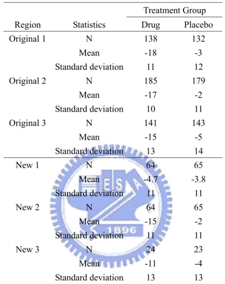
Hypothetical datasets modified from our review experience of bridging studies are used to illustrate the proposed procedure. The CCDP provides the results of three randomized, placebo controlled trials for a new anti-hypertension (test drug) conducted in the original region. The design, inclusion, exclusion criteria, dose, and duration of these three trials are similar, and hence the three trials constituted as the pivotal trials for approval in the original region. The primary endpoint is the change from baseline of sitting diastolic blood pressure (mmHg) at week 12. Because the regulatory agency in the new region still has some concerns in ethnic differences, both intrinsically and extrinsically, a bridging study was conducted in the new region to

compare the difference in efficacy between the new and original region. There are three scenarios to be considered. The first scenario presents the situation where no statistically significant difference in the primary endpoint exists between the test drug and placebo (2-sided p-value = 0.6430). The second situation is that the mean reduction of sitting diastolic blood pressure at week 12 of the test drug is statistically significantly greater than the placebo group (2-sided p-value < 0.0001). The third scenario is the situation where due to the insufficient sample size of the bridging study, no statistical significance is found between the test drug and placebo although the magnitude of the difference between the test drug and placebo observed in the original region is preserved in the new region (2-sided p-value = 0.0716). The number of patients and mean reduction and standard deviations of sitting diastolic blood pressure are provided in Table 2. The three scenarios are denoted as New 1 (Scenario 1), New 2 (Scenario 2), and New 3 (Scenario 3), respectively. The alternative hypothesis of interest is that the difference in change from baseline in sitting diastolic blood pressure at week 12 between the test drug and placebo is less than 0.

For the three original trials, the differences in mean reduction of sitting blood pressure between the test drug and the placebo are respectively 15mmHg, 15mmHg and 10mmHg. Also the pooled standard deviations for the three original trials are 11.5, 10.5 and 13.51mmHg, respectively. By the results from Section 2, the reference set

) , , (ω₁ ω₂ ω₃ = w is given as follows: 71 . 10 1 =−

ω , ω₂ =−13.62 and ω₃ =−6.24. Consequently, ω =−10.19 and

64 . 15 =

λ .

For the three new bridging trials, the standardized results, v, are -0.46, -6.71 and -1.85, respectively. In addition, the values of _(v−ω)2 _{are 94.59, 12.1 and 69.64,}

respectively. Regardless of the choice of ρ, the values of _(v−ω)2 _{are always are}

greater than −2( +1)lnρ+λ

K K

for the Scenario 1 and the Scenario 3 bridging trials. That is, we can not conclude that the results of the new region are similar to those of the original region for the Scenario 1 and the Scenario 3 bridging trials. On the other hand, for ρ≦3.77, the values of _(v−ω)2 _{are always are less than}

λ ρ+ + −2( 1)ln K K

for the Scenario 2 bridging trial. In this case, our procedure can prove the similarity of efficacy between the new and the original region.

At the design stage for the bridging trial, we may borrow the results from the original trials to determinate the sample size. From the three original trials in Table 1, we can obtain that w=(−15,−15,−10) , ω =−13.33 , 58_Σ2 ₌0. _and

097 . 0 } 097 . 0 , 34 . 0 , 36 . 0 min{ 0 = =

p . Table 2 provides the number of sample size

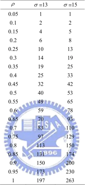
required per treatment group for the bridging study given γ =0.95, σ =13 and 15, respectively. It can be seen from Table 2 that the sample size increases as ρ increases. This makes intuitive sense, since the consistency trend required is stronger as ρ increases .

Example 2

After conducting successful original trials, we have observed that patients can be classified into two mutually exclusive genomic subgroups: those who are classified as marker positive (g+) and those classified as marker negative (g-). While the overall treatment effect was significant for the original trials, there might be two situations presented for the two mutually exclusive genomic subgroups.

Case II : the treatment effect exists in both subsets. However the magnitude of treatment effect in g+ is greater than that in g-.

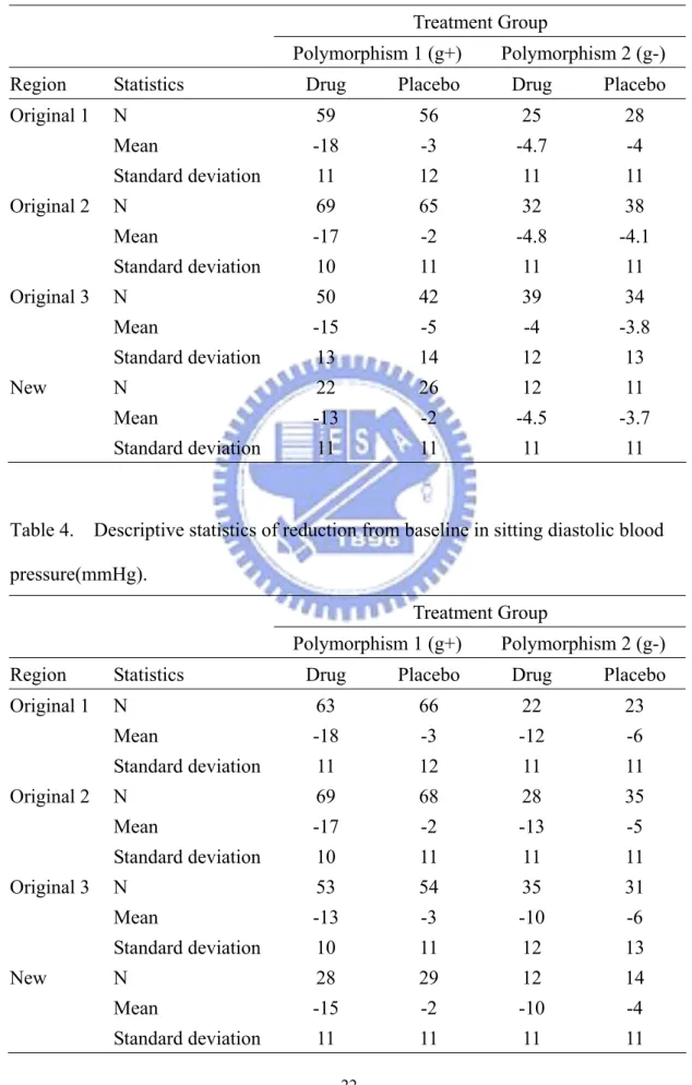
Following the design of clinical trials conducted in Example 1, Table 3 displays an example for Case I. In the three original trials, the differences in mean reduction of sitting blood pressure in g+ patient subgroup between the test drug and the placebo are respectively 15mmHg, 15mmHg and 10mmHg. However in the g- patient subgroup, the difference in mean reduction of sitting blood pressure between the test drug and placebo is 0.7mmHg , 0.7mmHg and 0.2mmHg, respectively. That is, the treatment effect may only exist in the g+ patient subgroup. For the first original trial, by (9) and (10), we can derive that ' 10.22

1 =− ω , 06var( ') 3. 1 = ω and * 5.84 1 =− ω .

Similarly, the observed standardized test statistics for the second original trial and the new bridging trial are respectively * 6.96

2 =−

ω , 6* 2.

3 =−

ω and _v* ₌₋2.94 _. Therefore, )* ₌(₋5.84,₋6.96,₋2.6

w and ω* =−5.14. Also, λ* =6.41. In this case,

(12) will hold if ρ is less than 1.8.

Alternatively, Table 4 presents an example for Case II. For the two original trials, the differences in mean reduction of sitting blood pressure for the patients in the g+ subgroup between the test drug and the placebo are 15mmHg, 15mmHg and 10mmHg, respectively. For the patients in the g- subgroup, the differences in mean reduction of sitting blood pressure between the test drug and placebo are 6mmHg, 8mmHg and 4mmHg, respectively. Again, by (9) and (10), we can derive that

25 . 7 * 1 =− ω , 58* 8. 2 =− ω , 82* 4. 3 =− ω and _v*₌₋4.47 _{. Hence,} ) 82 . 4 , 57 . 8 , 25 . 7 ( * _{= − − −}

can conclude that the results of the new region are similar to those of the original region if ρ is less than 0.56.

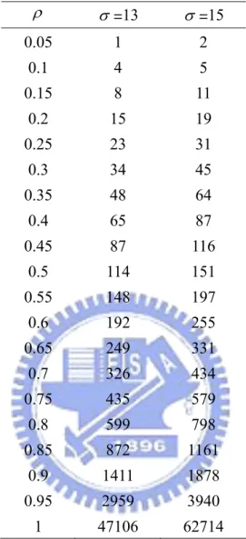
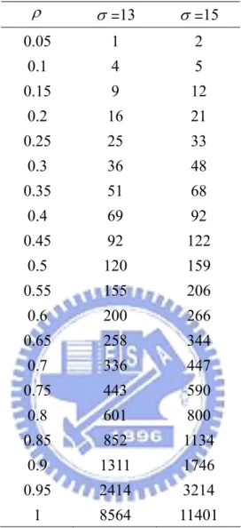
At the design stage for the bridging trial, we may borrow the results from the original trials to determinate the sample size. From the three original trials in Table 3 and Table 4, Table 5 and 6 display the number of sample size required per treatment group for the bridging study given γ =0.95 with σ =13 and 15, respectively. Again, it can be seen from both tables that the sample size increases as ρ increases. However, when ρ is large, conducting a bridging study may not be feasible.

5. Discussion

In this paper, we have proposed a statistical methodology for assessment of bridging evidence. More specifically, the similarity criterion is established by using the method of Bayesian most plausible prediction. Since reference studies from original region have already shown efficacy and safety, the concept of consistency is based on statistical prediction instead of conventional significance testing. With this approach, the total sample size might be reduced. That is, shortening the total duration of drug development may be possible.

Another point we wish to make is that the more diverse the previous results were, the larger the chance that the new trial would be consistent with (cf. (6)). That is, the results from new region more likely fall within the experience of the reference studies. However, the key constraint of conducting a bridging study in the new region is that the overall result of the reference studies must have already been shown

favorable to the test drug. It is obvious that when the variability is large, it is more difficult to show an overall favorable result for the test drug for the original trials. This requirement of showing a favorable overall result in effect places an upper bound on the variability, hence balances the degree of diversity that previous results may have.

Selection of the magnitude, ρ, of consistency trend may be critical. It may be determined by the regulatory agency in the specific region. All differences in ethnic factors between the specific region and other regions should be taken into account. However, the determination of ρ will be and should be different from product to product, from therapeutic area to therapeutic area and from region to region.

References

Aitchison J, Dunsmore IR. Statistical Prediction Analysis. Cambridge: Cambridge

University Press; 1975

Caraco Y. (2004). Genes and the response to drugs. The New England Journal of

Medicine, 351(27), 2867-9.

Chow, S. C., Shao, J., and Hu, O.Y. P. (2002). Assessing sensitivity and similarity in bridging studies, Journal of Biopharmaceutical Statistics, 12, pp. 385-400.

Hsiao C.F., Hsu Y.Y., Tsou H.H., and Liu J.P. (2007). Use Of Prior Information For Bayesian Evaluation Of Bridging Studies. Journal of Biopharmaceutical

Statistics, 17: 109–121.

ICH, International Conference on Harmonisation. (1998). Tripartite Guidance E5

Ethnic Factors in the Acceptability of Foreign Data. The U.S. Federal Register,

Lan, K. K., Soo, Y., Siu, C. Wang, M. (2005). The use of weighted Z-tests in medical research, Journal of Biopharmaceutical Statistics, 15(4), pp. 625-639.

Liu, J. P., Hsiao, C. F., and Hsueh, H. M. (2002). Bayesian approach to evaluation of bridging studies, Journal of Biopharmaceutical Statistics, 12, pp. 401-408. Liu, J. P., Hsueh, H. M., and Chen, J. J. (2002). Sample size requirement for

evaluation of bridging evidence, Biometrical Journal, 44, pp. 969-981. Pettiti, D. B. (2000). Meta-Analysis, Decision Analysis, and Cost-Effectiveness

Analysis. New York: Oxford University Press, pp. 90-129.

Shih, W. J. (2001). Clinical trials for drug registration in Asian-Pacific countries: proposal for a new paradigm from a statistical perspective. Controlled Clinical

Trials 22:357-366.

Zellner A. An Introduction to Bayesian Inference in Economics. New York: John

List of Tables

Table 1. Descriptive statistics of reduction from baseline in sitting diastolic blood pressure(mmHg).

Treatment Group

Region Statistics Drug Placebo

Original 1 N 138 132 Mean -18 -3 Standard deviation 11 12 Original 2 N 185 179 Mean -17 -2 Standard deviation 10 11 Original 3 N 141 143 Mean -15 -5 Standard deviation 13 14 New 1 N 64 65 Mean -4.7 -3.8 Standard deviation 11 11 New 2 N 64 65 Mean -15 -2 Standard deviation 11 11 New 3 N 24 23 Mean -11 -4 Standard deviation 13 13

Table 2. The number of sample size required per treatment group for the bridging study given γ =0.95. ρ _{σ =13 σ =15} 0.05 1 1 0.1 2 2 0.15 4 5 0.2 6 8 0.25 10 13 0.3 14 19 0.35 19 25 0.4 25 33 0.45 32 42 0.5 40 53 0.55 49 65 0.6 59 78 0.65 70 93 0.7 83 110 0.75 97 129 0.8 113 150 0.85 131 174 0.9 150 200 0.95 173 230 1 197 263

Table 3. Descriptive statistics of reduction from baseline in sitting diastolic blood pressure(mmHg).

Treatment Group

Polymorphism 1 (g+) Polymorphism 2 (g-)

Region Statistics Drug Placebo Drug Placebo

Original 1 N 59 56 25 28 Mean -18 -3 -4.7 -4 Standard deviation 11 12 11 11 Original 2 N 69 65 32 38 Mean -17 -2 -4.8 -4.1 Standard deviation 10 11 11 11 Original 3 N 50 42 39 34 Mean -15 -5 -4 -3.8 Standard deviation 13 14 12 13 New N 22 26 12 11 Mean -13 -2 -4.5 -3.7 Standard deviation 11 11 11 11

Table 4. Descriptive statistics of reduction from baseline in sitting diastolic blood pressure(mmHg).

Treatment Group

Polymorphism 1 (g+) Polymorphism 2 (g-)

Region Statistics Drug Placebo Drug Placebo

Original 1 N 63 66 22 23 Mean -18 -3 -12 -6 Standard deviation 11 12 11 11 Original 2 N 69 68 28 35 Mean -17 -2 -13 -5 Standard deviation 10 11 11 11 Original 3 N 53 54 35 31 Mean -13 -3 -10 -6 Standard deviation 10 11 12 13 New N 28 29 12 14 Mean -15 -2 -10 -4 Standard deviation 11 11 11 11

Table 5. The number of sample size required per treatment group for the bridging study given γ =0.95. ρ _{σ =13 σ =15} 0.05 1 2 0.1 4 5 0.15 8 11 0.2 15 19 0.25 23 31 0.3 34 45 0.35 48 64 0.4 65 87 0.45 87 116 0.5 114 151 0.55 148 197 0.6 192 255 0.65 249 331 0.7 326 434 0.75 435 579 0.8 599 798 0.85 872 1161 0.9 1411 1878 0.95 2959 3940 1 47106 62714

Table 6. The number of sample size required per treatment group for the bridging study given γ =0.95. ρ _{σ =13 σ =15} 0.05 1 2 0.1 4 5 0.15 9 12 0.2 16 21 0.25 25 33 0.3 36 48 0.35 51 68 0.4 69 92 0.45 92 122 0.5 120 159 0.55 155 206 0.6 200 266 0.65 258 344 0.7 336 447 0.75 443 590 0.8 601 800 0.85 852 1134 0.9 1311 1746 0.95 2414 3214 1 8564 11401