基於偵幅複雜度畫面內編碼在H.264的位元率控制演算法

國立交通大學

多媒體工程研究所

碩士論文

基於偵幅複雜度畫面內編碼在 H.264 的位元率控制演

算法

A H.264 intra-frame rate control based on frame

complexity

研究生：許智為

指導教授：蔡文錦 博士

基於偵幅複雜度畫面內編碼在 H.264 的位元率控制演算法

A H.264 intra-frame rate control based on frame complexity

研 究 生：許智為 Student：Chih-Wei Hsu

指導教授：蔡文錦 Advisor：Wen-Jiin Tsai

國 立 交 通 大 學

多 媒 體 工 程 研 究 所

碩 士 論 文

Submitted to Institute of Multimedia Engineering College of Computer Science

National Chiao Tung University in partial Fulfillment of the Requirements

for the Degree of Master

in

Computer Science

June 2010

Hsinchu, Taiwan, Republic of China

中文摘要

為了讓視訊編碼後的位元率能維持在頻寬的限制之內，並且達到良好與穩定 的畫面品質，位元率控制是相當重要的。然而目前大多數的研究都集中在畫面間 編碼(inter frames)而不是容易造成緩衝區溢位的畫面內編碼(intra frames)。此外 Intra-only 這種編碼方式也已經納入 H.264 新的 profile 當中，它較傳統 GOP 編碼更 適合應用在特別要求畫面品質的產品上。 在此論文中，我們提出一個於 Intra-only 編碼的位元率控制演算法。首先我們 提出基於 R-D-Q model 最佳化的 QP 決定方式，藉由位元率與 PSNR 預測模型，我 們利用 R-D-Q model 最佳化來找出可以平衡畫面品質與編碼效能的 QP 最佳解。另 外，在 Intra-only 編碼上為了解決場景變換對位元率控制所產生的影響，我們所利 用的 R-D-Q model 可以直接偵測場景變換並做適當 QP 選擇，避免緩衝區溢位。實 驗結果顯示，提出的方法可以達到更好更穩定的畫面品質，且緩衝內含量也都維 持在較低的水平。 關鍵字： 位元率控制、H.264、畫面內編碼、R-D-Q model、預測模型

ABSTRACT

Rate control serves as an important technique to constrain the bit rate of video transmission over a limited bandwidth and to control the bit allocations within a video sequence to maximize its overall visual quality. However, most of rate control researches focus on inter coding frames instead of intra coding frames which are more possible to cause buffer overflow problem. Besides, H.264 Intra-only compression scheme has been standardized as H.264 profiles which are more proper for professional applications than traditional GOP compression scheme.

In this thesis, we propose an improved rate control scheme which is appropriate for Intra-only compression. First, we present a R-D-Q model based QP determination scheme for I-frames and P-frames . By the estimation models for rate and PSNR of I-frames, the best quantization parameters can be determined by R-D-Q model method. In order to deal with the specific intra frames caused by scene transitions, our R-D-Q model can directory detect scene change without extra detection to determine appropriate QPs for avoiding buffer overflow and saving bit budget. Simulation results show, that compared to other reference algorithms, our approach achieves better and stable quality with low buffer fullness.

CONTENTS

中文摘要 ... i

ABSTRACT ... ii

CONTENTS ... iii

LIST OF FIGURES ... v

LIST OF TABLES ... vii

Chapter 1 Introduction and Motivation ... 1

1.1 Introduction to Rate Control ... 1

1.1.1 The Chicken Egg Dilemma for H.264 Rate Control ... 3

1.1.2 Main Criteria of Rate Control ... 4

1.2 Introduction to H.264 Intra-coded Frames ... 5

1.2.1 H.264 Intra Compression ... 6

1.2.2 H.264 Intra-only Profiles... 6

1.3 Motivation ... 7

Chapter 2 Related Works ... 10

2.1 G012 Rate Control for H.264 ... 10

2.1.1 Terminology ... 10

2.1.2 Overview to G012 Rate Control ... 13

2.2 Source Model for Transform Video Coder and Its Application-Part I: Fundamental Theory ... 15

2.3 Cauchy Density based Rate Control for H.264 ... 17

2.4 Frame Complexity based Intra only Rate Control ... 19

2.5 Effective Intra-only Rate Control for H.264/AVC ... 20

2.6 Summary ... 22

Chapter 3 Proposed Rate Control Algorithm for Intra-only Compression ... 24

3.1 R-D-Q Model ... 24

3.1.1 Estimation of E’ ... 25

3.1.2 Estimation of D ... 27

3.1.3 Estimation of α ... 28

3.1.4 QP Determination Method for Intra Frames ... 31

3.2 Description of the Proposed Rate Control Algorithm for Intra-only Compression ... 32

3.2.2 QP refinement Algorithm ... 32

3.2.3 Proposed Rate Control Algorithm ... 34

3.2.4 Proposed Rate Control Algorithm Verification ... 35

Chapter 4 Experiment Results ... 40

4.1 Results of Intra-only Compression ... 41

Chapter 5 Conclusion ... 56

LIST OF FIGURES

Fig 1-1 Video transmission system ... 2

Fig 1-2 (a) Variable bit rate vs. (b) Constant bit rate ... 3

Fig 1-3 Basic rate control flow ... 3

Fig 1-4 The chicken egg dilemma for H.264 rate control ... 4

Fig 1-5 4x4 block intra prediction mode direction[9] ... 6

Fig 1-6 (a) JM’s MAD predict and actual curve (b) Jing’s a predict and actual curve @ test sequence scene change(SC) pre 10 frame ... 9

Fig 2-1 The G012 rate control diagram ... 13

Fig 2-2 Comparison of Laplacian model vs. Cauchy model[16] ... 18

Fig 2-3 Intra coded bits vs. gradient per pixel (a) Foreman, QP=36 (b) Carphone, QP=25 ... 19

Fig 2-4 R-Q relation ... 20

Fig 2-5 relationship between R and GeoGrad ... 21

Fig 2-6 The relation between SCI and general I-frames ... 23

Fig 3-1: the relation of E and QS @news qcif, foreman qcif, highwayqcif, foreman CIF, crew SD, shield HD from frame#2 to frame#6 ... 26

Fig 3-2 : E term prediction error from frame#2 to frame#6 ... 27

Fig 3-3 the relation of PSNR and QS in different sequences from frame#2 to frame#6 28 Fig 3-4 linear relation between QP and alpha term after processing from frame#2 to frame #6... 29

Fig 3-5 different resolution alpha term ... 30

Fig 3-6 shows the predict alpha term and actual alpha term ... 31

Fig 3-7 diagram of the proposed QP determination model ... 32

Fig 3-8 Flow charts for Intra-only compression ... 34

Fig 3-9 football QCIF model verification at QP+4 ... 35

Fig 3-10 football QCIF model verification at QP+3 ... 36

Fig 3-11 football QCIF model verification at QP+2 ... 36

Fig 3-12 football QCIF model verification at QP1 ... 37

Fig 3-13 football QCIF model verification at QP-4 ... 38

Fig 3-14 football QCIF model verification at QP - 3 ... 38

Fig 4-1 PSNR v.s. frames (a) carphone QCIF (b) combo_CIF_3 (c) combo_CIF_1 (d) combo_SD (e) combo_HD ... 51 Fig 4-2 Buffer fullness v.s. frames (a) carphone QCIF (b) combo_CIF_3 (c) combo_CIF_1 (d) combo_SD (e) combo_HD ... 55

LIST OF TABLES

Table 1-1 Comparison between Intra-only and GOP compression[10] ... 7

Table 3-1 the correlation of test sequence ... 26

Table 3-2 the correlation of PSNR and QS ... 28

Table 3-3 the correlation between QP and predict alpha term ... 30

Table 3-4 different resolution multiply ... 31

Table 4-1 test sequences ... 40

Table 4-2 QCIF Preference Result (a) Bit rate and Average PSNR (b) PSNR standard derivation ... 43

Table 4-3 CIF Preference Result (a) Bit rate and Average PSNR (b) PSNR standard derivation ... 45

Table 4-4 SD Preference Result (a) Bit rate and Average PSNR (b) PSNR standard derivation ... 47

Table 4-5 HD Preference Result (a) Bit rate and Average PSNR (b) PSNR standard derivation ... 49

Chapter 1

Introduction and Motivation

For the coming of digital multimedia communication, the demand for the storage and transmission of visual information has stimulated the development of video coding standards, including MPEG-1[1], MPEG-2[2], MPEG-4[3], H.261[4], H.263[5], and H.264/AVC[6].

H.264 is an up-to-date coding standard approved by ITU-T as MPEG 4 - Part 10 Advanced Video Coding (AVC). It includes the latest advances of video coding techniques. H.264 is designed in two layers: a video coding layer (VCL), and a network adaptation layer (NAL). Although H.264/AVC basically follows the framework of prior video coding standards such as MPEG-2, H.263, and MPEG-4, it contains new features that enable it to achieve a significant improvement in compression efficiency.

1.1

Introduction to Rate Control

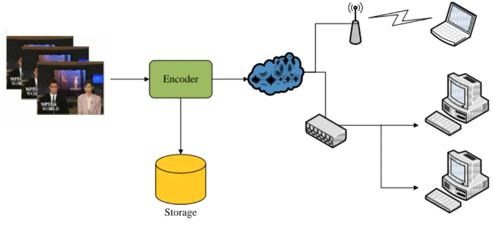
A rate control algorithm which meets a constrained channel rate by controlling the number of generated bits is necessary to encoder. Either the coded video is transmitted over the Internet or stored in a storage device; there is a bandwidth constraint to limit the bit rate of videos. Although the transmission bandwidth is growing larger over the years, more exquisite videos with high resolutions, such as HD and Full HD, are becoming popular. These high definition videos consume much more bit rate than the traditional definition videos. Encoding video without rate control will suffer from several serious problems. For example, when the coded video transmits through a weak wireless access point (AP), network congestion and packet loss will occur if the bit rate of the video is higher than the bandwidth of the AP. In another example, suppose the generated bits are not constrained carefully, the fact that out of storage capacity will

happen. Fig 1-1 shows the two mentioned examples. Hence, rate control is a key issue of the modern video coding researches.

The generated bits and video quality of an encoder highly rely on several coding parameters, especially the quantization parameter (QP). In particular, choosing a large QP reduces the resulting bit rate and meanwhile the visual quality of the encoded video is reduced. For illustration, Fig 1-2(a) shows that if the QP is constant, the resulting video is at a stable quality with a variable bit rate (VBR). However, a predetermined constant bit rate (CBR) is desired in most applications, such as CD, DVD, or video broadcast. Fig 1-2(b) shows the quality of a coded video with CBR floats because of the

video content varying.

Encoder

Storage

Fig 1-1 Video transmission system

Time P S N R Time R a te Time P S N R Time R a te

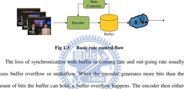
The task of controlling output bit rate by selecting an appropriate quantization parameter for each coding unit is performed by the rate control module. The goal of rate control is to keep the generated bit rate within the constrained bandwidth while achieving maximum video quality uniformly. A simple approach of rate control is shown in Fig 1-3. Basically, the encoder buffer smoothes out the bit rate so that the averaged output bit rate matches the channel bit rate.

The loss of synchronization with buffer in-coming rate and out-going rate usually causes buffer overflow or underflow. When the encoder generates more bits than the amount of bits the buffer can hold, a buffer overflow happens. The encoder then either re-encodes the current frame with coarser QP or simply drops it (frame skip) to avoid the overflow. A buffer underflow is the situation while there is no bit available in the encoder buffer. It wastes the available channel bandwidth. By monitoring the status of buffer, the rate controller can adjust the quantization parameters, which affects the output bit rate, to prevent the buffer from overflow and underflow.

1.1.1 The Chicken Egg Dilemma for H.264 Rate Control

One important property of H.264 is the implementation of rate distortion optimization (RDO)[7] for both motion estimation and mode decision. With RDO, the Lagrangian method is utilized to optimize the trade-off between distortion and bit rate consumed. For example, the Lagrangian cost function of motion estimation[7] is

Fig 1-2 (a) Variable bit rate vs. (b) Constant bit rate

Buffer Rate

Controler

Encoder



,

|

,





,

|





,

|



Motion i i i i i i

J

MB MV QP





D MB MV QP

 



R MB MV QP

(1-1)

where

MB

MV

of ith MB in the current frame, respectively; λ denotes the Lagrangian multiplier

which depends on

 12 3

0.85 2QP



(1-2)

According to (1-1) and (1-2), the cost calculation for each MV of the current MB takes QP as an important input parameter.

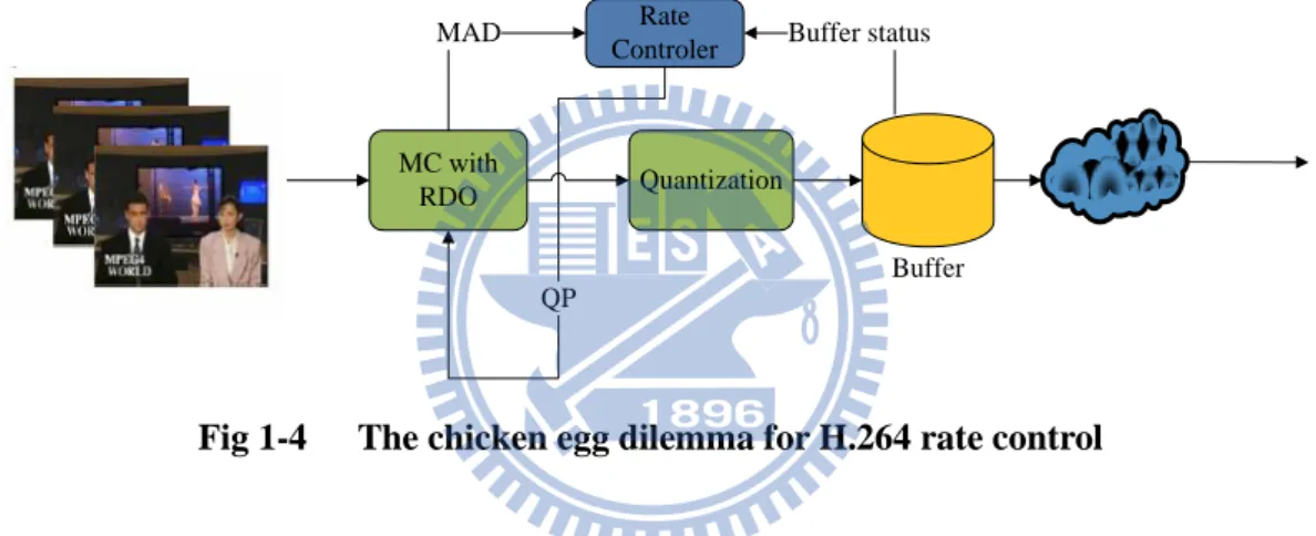
Therefore, in H.264, QP affects both rate distortion optimization and residual quantization. In this way, the statistical information of the residual frame, such as mean absolute difference (MAD), varies with the QP adjustment, and the QP decision is also influenced by the statistical information. As shown in Fig 1-4, the rate control unit requires the MAD value from RDO to determine the QP value, but the RDO procedure also needs QP as an input parameter. This is the chicken egg dilemma for H.264 rate control.

1.1.2 Main Criteria of Rate Control

Rate control algorithms concentrate on keeping the encoded video quality as consistent and excellent as possible for each frame and constraining the bit rate within

Buffer status Buffer Rate Controler QP Quantization MC with RDO MAD

rate control:

A. Mismatch between the target bit rate and the output bit rate.

Because the main purpose of rate control is to constrain the output bit rate within the target bit rate, the mismatch between both should be minimized.

B. Average PSNR of whole sequence.

The generated video quality should be at the highest possible level for a better watching experience.

C. Standard deviation of PSNR between frames.

This criterion implies the quality variation of the video produced by the rate control algorithm. A good rate control should keep the deviation low, i.e., keep the quality variation small.

D. Maximum buffer fullness.

Lower maximum buffer occupancy implies that a small buffer is sufficient for preventing from buffer overflow. Further, a small buffer only takes few buffer delay while transmission. A good rate control algorithm should minimize the maximum buffer fullness.

1.2

Introduction to H.264 Intra-coded Frames

H.264 exploits both temporal and spatial redundancy to increase its coding gain. It supports intra prediction mode to exploit the spatial domain correlation which helps reduce the residual energy of intra frames.

Recently, H.264 intra-only coding scheme for professional applications has been standardized as H.264 profiles[8]. These intra-only profiles take the advantages of H.264 intra coded frames and make H.264 as another great selection for intra compressed video.

1.2.1 H.264 Intra Compression

H.264 utilizes the intra prediction to reduce the spatial redundancy within frames. Fig 1-5 shows the prediction options of 4x4 block intra prediction. Each pixel in the current 4x4 block is predicted from the neighboring reconstructed pixels, where nine prediction modes can be selected by the encoder, and the residue between the current block and the predicted block will be quantized for entropy coding. The key to the success of intra coding on improving the performance is that the entropy of the residual block is much less than the original block. Hence, the coding gain after intra prediction will be significantly superior.

1.2.2 H.264 Intra-only Profiles

In the seventh edition specification of H.264, there are three new profiles, e.g.,

High 10 Intra, High 4:2:2 Intra, and High 4:4:4 Intra, which are designed for

professional applications. For the reason that the intra-only profile does not exploit the temporal correlation, there is no temporal dependency between consecutive frames. It is more convenient for editing and parallel processing, even less error propagation. Table 1-1 summaries the differences between intra-only scheme and the standard GOP compression. Because of the features of intra-only compression, it is greatly appropriate for the high-end applications.

Table 1-1 Comparison between Intra-only and GOP compression[10]

1.3

Motivation

Rate control aims at providing highest possible video quality while satisfying the limited bandwidth. Although various rate control algorithms have been proposed for H.264 (see Chapter 2), most of them focus on inter coding instead of intra coding, because the output number of bits of an intra coding frame is much higher than that of an inter frame. It is also more possible that the intra coded frame causes buffer overflow when the generated bits exceed the amount of bits that buffer can hold.

In the H.264 original rate control algorithm[11], the QP for each I-frame is decided by the average QP of all coded P-frames in the previous GOP. This approach does not take the buffer status and the frame complexity into consideration, and usually allocate too much bits for the I-frame, which degrades the video quality of the following

Intra-only Compression GOP Compression

Compression scheme

Bit rate saving Smaller Use spatial correlation only

Greater Use spatial and temporal correlations

Process delay Smaller 1 frame Greater Multiple frames

Edit easiness Easier frame by frame More difficult GOP

Error

propagation

Smaller Max. 1 frame Greater Multiple frames

Parallel processing

Easier Frame independent

P-frames due to insufficient bits. In addition, because the intra coded DCT coefficients are not Laplacian distributed, the quadratic model which is used to predict the relation between bit rate and quantization parameter is not appropriate for intra frames.

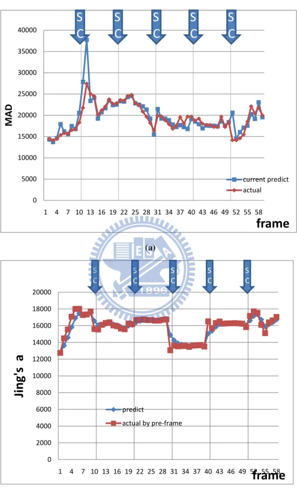
We observed that the QP determination by pre-frame information’s rate control algorithm would lead to the unpredictable result, for example the buffer overflow, PSNR drop, and the PSNR standard derivation larger, such as in more activity sequence or in the sequence which happened scene change often. Fig 1-6 shows the information predict by pre-frame. It really tells us the prediction by pre-frame in scene change shows the prediction error lager, which can lead to over of under estimation QP makes the generated bits larger or smaller than target bits.

Since most existing rate control algorithms for H.264 cannot handle the intra frames and scene change frames well, we need to find out a new scheme to determine the QPs for both kinds of frames. Instead of using the average QP of P-frames in the previous GOP, in this thesis, we propose an improved rate control algorithm that takes frame complexity into consideration to decide proper QPs for the intra frames.

The remainder of this thesis is organized as follows: Chapter 2 introduces the related researches about rate control issue. Chapter 3 presents the proposed rate control scheme for Intra-only compression. Chapter 4 provides the simulation results compared to other rate control schemes. Finally, Chapter 5 concludes this thesis.

(a)

(b)

Fig 1-6 (a) JM’s MAD predict and actual curve (b) Jing’s a predict and actual curve @ test sequence scene change(SC) pre 10 frame

0 5000 10000 15000 20000 25000 30000 35000 40000 1 4 7 10 13 16 19 22 25 28 31 34 37 40 43 46 49 52 55 58

MAD

frame

S

C

S

C

S

C

S

C

S

C

Ji

n

g's

a

frame

Chapter 2

Related Works

Rate control techniques have been studied intensively for many standards. The challenge of rate control in video encoding is to determine an appropriate quantization parameters to achieve the best video quality within the given application constraints. In this chapter, we will introduce the most famous rate control algorithm which is adopted in the official reference coding software of H.264[12] and other improved schemes for H.264 intra rate control.

2.1

G012 Rate Control for H.264

Li et al. proposed an one pass rate control algorithm, JVT-G012[11], which used the rate-quantization (R-Q) quadratic model in the standard MPEG4 rate control, and introduced the linear mean absolute difference (MAD) prediction model to solve the dilemma that we have mentioned in the previous chapter. Due to its efficiency, this scheme was adopted by JVT in the latest H.264 reference software.

2.1.1 Terminology

Before we introduce this algorithm, there are three terminologies we have to mention first.

A. Definition of A Basic Unit

Suppose that a frame is composed of N_mbpic macroblocks (MBs). A basic unit is

defined as a group of continuous MBs which is composed of

N

where

N

picunit unit mbunit N N N  (2-1)

A basic unit can be selected as a frame or some consecutive MBs. Note that, a smaller basic unit is needed in some low-delay applications which require stricter buffer regulations, less buffer delay, and better spatially perceptual quality. However, it is costly at low bit rate since there is additional overhead if the quantization parameter is varying frequently within a frame. On the other hand, by using a bigger basic unit, a higher PSNR can be achieved but the bit fluctuation is also larger.

B. Linear Model for MAD Prediction

MAD is the mean absolute difference between the reference frame and the current frame which describes the residue information and is given by

 











where C and

R

In order to solve the chicken egg dilemma in H.264 rate control, the linear model is used to predict the MADs of the basic units in the current frame by using the MADs of the co-located basic units in the previous frame. The linear prediction model is then given by

1 2

pb cb

MAD  a MAD a

(2-3)

where

a

a

cb

MAD stand for the predicted MAD of the current basic unit and the real MAD of the co-located basic unit, respectively. The initial values of

a

a

respectively. They are updated after each basic unit has been encoded.

In order to illustrate the quadratic rate distortion model, we summarize the results in [13][14]. Assume that the source statistics satisfy a Laplacain distribution

( ) where 2

x

P x 



(2-4)

and the distortion measure is defined by,

D x x

( , )

 

x x

sample and x is the reconstruction of x. Then, a closed solution for R-D function was

derived as min max 1 1 1 ( ) ln where 0, ,0 R D D D D D







Based on the R-D function, a quadratic rate-control model was proposed in [13] as

1 2 2 X X R QP QP   (2-6)

where R is the target number of bits used for encoding the current frame, and

X

2

X

previous coded information.

Lee et al.[14] improved the model with content scalability and achieved more accurate bit allocation within limited target bits. The improved model has been adopted as a part of the MPEG4 standard, and known as MPEG4 Q2 algorithm. The quadratic rate distortion model is defined by

1 2 2 MAD X MAD X R H QP QP      (2-7)

where

H

MAD

accomplishing the scalability of this model.

2.1.2 Overview to G012 Rate Control

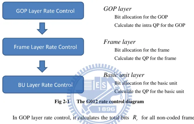
As shown in Fig 2-1, G012 partitioned the rate control problem into three layers: 1) GOP layer; 2) frame layer, and 3) basic unit layer. There are two sub-problems, bit allocation and QP determination, for each layer.

In GOP layer rate control, it calculates the total bits

R

within the current GOP, and selects the QP for the starting I-frame. In the beginning of each GOP, the total number of bits is computed as follows

r GOP c r u R N B F    (2-8)

where u is the channel bit rate;

F

N

number of frames in a GOP, and

B

previous frame. In the case of constant bit rate,

R

r r

R



R



b

(2-9)

Fig 2-1 The G012 rate control diagram

GOP layer

Bit allocation for the GOP

Calculate the intra QP for the GOP

Frame layer

Bit allocation for the frame Calculate the QP for the frame

Basic unit layer

Bit allocation for the basic unit Calculate the QP for the basic unit

where b is the number of bits generated from the previous coded frame.

The starting QP of the first GOP, QP_{I first,} depends on the channel bit rate and the

value of bit per pixel (bpp). On the other side, the starting QP of other GOPs, QP_{I other,}

is determined as the average QP of the P-frames of the previous GOP. Summarily, the starting QP is selected as follows

1 1 2 , 2 3 3 4 , 40 30 , 20 10 I first r pixel I other p bpp l l bpp l _u QP where bpp l bpp l F N l bpp l SumQP QP N      _{ }   _{ }  _{  }  _  _{  }       (2-10)

where N_pixel is the number of pixels within a frame; N_p indicates the number of P-frames of a GOP, and SumQP stands for the summation of QPs of all P-frames of the previous GOP.

l

The approach of frame layer involves distributing the GOP budget among the frames and determines the QP of each frame to achieve the allocated budget. The target number of bits of ith P-frame in the current GOP is determined as





ˆ ₁

i i i

R    





(2-11)

where



R

ˆ

R

ˆ r i remain R R N  (2-12)







where

N



Tbl

V

frame, respectively.

After accomplishing the bit allocation, the linear MAD prediction model (2-3) and the quadratic rate distortion model (2-7) are utilized to determine the QP of the current frame, and then RDO procedure is performed for mode decision. At the last, the parameters of the quadratic model, and those of the MAD prediction model are updated based on the coding results.

If frames are not selected as basic units, basic unit layer rate control should be performed after frame layer bit allocation. In basic unit layer, it is almost the same as that in frame layer. It predicts MADs of all basic units in the current frame by equation (2-3) and calculates the target number of bits of them by

2 , , 2 , unit i pred i c remain N j pred j i MAD b R MAD   



where R_{c remain,} is the remaining target number of bits of current frame; MAD_{i pred,}

stands for the predicted MAD of ith basic unit in the current frame. Then, the quadratic

model (2-7) is proposed to determine the QP of the current basic unit.

2.2

Source Model for Transform Video Coder and Its

Application-Part I: Fundamental Theory

A source model describing the relationship between bits, distortion, and quantization step sizes of a large class of block-transform video coders is proposed in [15]. This model is initially derived from the rate-distortion theory and then modified to match the practical coders and real image data. The realistic constrains such as quantizer

dead-zone and threshold coefficient selections are included in Hang’s formulation. The most attractive feature of this model is its simplicity in its final form. Its enables us to predict the bits needed to encode a picture at a given distortion or to predict the quantization step size at a given bit rate.

The well known rate distortion function of a discrete stationary Gaussian process {x(n)} under the mean square distortion criterion is given as:

               







where Φ(ω) is the power spectrum density function of {x(n)}. That is Rθ is the

minimum bit necessary to achieve an average distortion D by an ideal coder of possibly unbounded complexity and time delay. D(R) is the minimum average distortion that can possibly be achieved at bit rate R. In reality, we cannot use infinite length transforms to decompose a signal sequence in to non-overlapped block and perform block

transformation on each data block separately. Then the simple and popular spectrum estimation method is the periodogram that computes the spectrum based on the weighted average of the Fourier transforms of non-overlapped data blocks . This data compression if the blocks transform components is the discrete approximation of the ideal continuous power spectrum. Assuming a uniform sampling grid in the frequency domain, the equation (2-15) can be approximated by the following discrete formula:







Hang’s shows that a case of interest is that at low distortion when A1 = (-π,π〕(or B1 is

empty) then D(Rθ) = θ. Then the equation (2-16) can be rewritten as:

L L i i E where D E D R 1 1 0 ) ( ln 1 ) (       _  



where L is the number of samples in a data block. The bits and distortion of a signal are decided by a single parameter E, which is the product of all the components’ variances. It represents the complexity of the signal. In theory, two signals of the same ordinary variance require different numbers bits of in coding if their E are significantly different.

2.3

Cauchy Density based Rate Control for H.264

Knowledge of the probability distribution of discrete cosine transform (DCT) coefficient is important in the design and optimization of rate control algorithms. In the early studies [16], the coefficients are conjectured to have Laplacian distribution. In [17], Kamaci et al. proposed a better solution using a Cauchy probability density function (pdf) for DCT coefficients estimation. As shown in Fig 2-2, Cauchy model actually outperforms traditional Laplacian model in both intra and inter coded frames.

Kamaci et al. further presented the Cauchy density based rate estimation models by approximating the entropy function of quantization. The rate model was applied in frame layer to determine the QP of each frame based on the given target number of bits of current frame

R

Their Cauchy based rate estimation models is

b

R a QS (2-18)

where QS is the quantization step; a and b are model parameters which depend on

the content of the coding sequence and different types of coding mode, i.e., I-, P-, and B-frames. Then, the QS is determined as following

b R QS

a

 (2-19)

Finally, the QP used for RDO can be calculated by



6



log

(

)



4





QS

QP

2.4

Frame Complexity based Intra only Rate Control

Based on Kamaci et al.’s rate estimation model, Jing et al.[18] proposed an improved model which is applied on intra frames and has sufficient adaptability to the varying of intra frame complexity.

In their proposed algorithm, they defined the complexity measure of intra frames as the average gradient per pixel of the frame. The calculation of gradient complexity is defined by 1 1 , 1, , , 1 0 0 1 M N i j i j i j i j i j G I I I I M N          _    _  



where

M

N

 

i j

,

(a)

(b)

Fig 2-3 Intra coded bits vs. gradient per pixel (a) Foreman, QP=36 (b) Carphone, QP=25

They observed that the number of coding bits of an intra coded frame is highly correlated with its gradient value, as shown in Fig 2-3. From the linear correlation

0.6 0.8 1 1.2 1.4 8 10 12 14 16 18 20 In tr a co d e d b its x 1000 0

Gradient per pixel

2.5 3 3.5 4 11 12 13 14 15 16 17 In tr a co d e d b its x 1000 0

between these two factors, they assumed that for a fixed QP, the output number of bits of one intra frame is proportional to the value of its average gradient per pixel. Based on the assumption, they revised Cauchy rate estimation model as follows

b

R  G a QS (2-22)

where b is a constant which is set to -0.8 and a is updated frame by frame as





0

1

R

k

G QS

a

R

a

otherwise

G

QS







_



_



 

 

 









After frame layer bit allocation, QS can be calculated by (2-23), and QP can be derived from (2-22).

2.5

Effective Intra-only Rate Control for H.264/AVC

In Tian’s proposed algorithm [19], they would like to increase the performance of intra-only rate control, so they introduces the geometry gradient information as a new complexity measure to accurately represent the complexity of an intra-frame and to develop a linear rate-complexity model. In their paper, a RD model also proposed.

The R-Q model with an exponential form as follows:

Q

e

R









The R-C model is also proposed, for intra-frames the motion estimation between consecutive frames is not required, and the output bits only relate to the content complexity of the intra-frame itself. In Tian’s paper, they proposed a new complexity measure called geometry gradient, to estimate the content complexity for a picture. The formula as follows:

 













)

1

)(

1

(

M

N

P

P

P

P

GeoGrad

where P is luminance value of a pixel, N and M denote the columns and rows of a frame. The Fig 2-5 shows the relationship between R and GeoGrad..

Fig 2-5 relationship between R and GeoGrad

The R-C model formula as follows:

b

G

a

R







) ( 1 ^ 1 1 1 ^ 1 ^ 1 1

)

,

(

)

(

)

,

(

5

.

0

ln

)

,

(

ln





































e

Q

G

R

A

and

G

G

a

R

Q

G

R

where

A

Q

G

R

Q

Q



where the β and a are update by pre-five frames by linear regression as following formula: 2 1 0 1 0 2 1 0 1 0 ~ 1 0 ~ 2 1 0 1 0 2 1 0 1 0 1 0

)

(

)

ln

)(

(

)

(

)

ln

)(

(

ln















































G

G

w

G

G

w

a

and

Q

Q

w

R

Q

R

Q

w

R

R



2.6

Summary

In the above sections, we have introduced several researches for H.264 rate control and intra coded frame rate control. However, they still have some problems which can be organized as follows:

A. Without Dealing with Scene Change Intra Frames

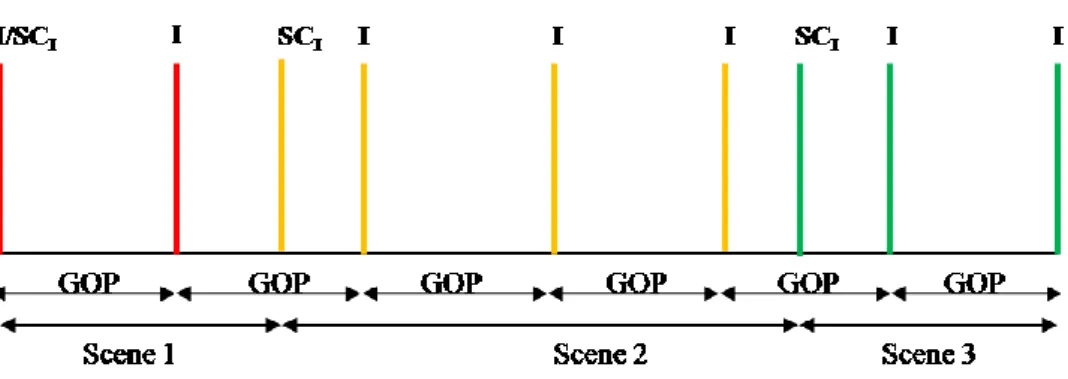
Due to that all MBs within a scene transition frame will be intra coded, we regard such a frame as a special kind of intra frame, called scene change intra frame (SCI). The

locations of SCI frames and general intra frames in a video sequence can be illustrated

Similar to general I-frames, these SCI can cause serious buffer overflow problem if

no appropriate QP is determined for them. Actually the prediction result in their model parameter even won’t get a reasonable result, like Fig 1-6 shows the prediction by pre-frame. Although rate control algorithms have been widely studied [11][17], most of them didn’t deal with the scene change intra frames.

B. No Accurate Rate Quantization Model for Intra Frames

The quadratic model (2-7) is designed for inter coded frames whose source statistics are assumed satisfying Laplacain distribution. However, this assumption is inappropriate to intra coded frames. Jing et al.[18] and Tian et al.[19] are proposed a novel rate quantization model for intra frames, but their parameter cannot be estimated precisely. In order to determine this parameter, they employed an update procedure which assumes that its value is stationary frame by frame. However, this assumption is not always true where the parameter value in the figure varies frequently.

Chapter 3

Proposed Rate Control Algorithm for

Intra-only Compression

This section presents the proposed rate control algorithm for intra-only compression. We first describe a rate-distortion-QS model for bit-rate prediction, and then a QP determination algorithm is proposed.

3.1

R-D-Q Model

The proposed R-D-Q model is based on Hang’s source model [15], formula (3-1), where E is the entropy variance of a signal, D is signal distortion, andα is a model parameter. D E D R( ) 1 log   _(3-1)

When applying to intra-only coding, we replace E with the E’ in equation (3-2), which represents the MSE between original pixel and residual value after intra prediction; replace D with the D’ in equation (3-3), which represents the MSE between original frame and reconstructed frame; and redefine R(D) as the bit-rate needed to encode this frame, subject to the distortion D’:





)

j)

f(i,

-j)

(f(i,

'

E'



From equations (3-2) and (3-3), it can be seen that both E’ and D’ depends on the reconstructed frame which is unknown before encoding, and therefore we need a way to estimate E’ and D’ accurately. And the f( ji, ) means original frame pixel, the (, )

~

j i f

frame. The estimates of E’ and D’ are presented in section 3.1.1 and section 3.1.2, respectively. The model parameter α subject to the re-defined E, D, and R is presented in section 3.1.3.

3.1.1 Estimation of E’

To estimate E’, experiments were conducted for various intra-coded sequences and finally we found that E’ value is a function of frame complexity (G), frame resolution (S), and quantization step size (QS). That is, E’= f(G, S, QS). The frame complexity, G, is measured using pixel gradient. Let

I i j

 

,

 

  



  



n

g i j  I i j I i j  I i j I i j _(3-4)

And the frame complexity of nth frame, say Gn, is defined by average gradient per pixel

of that frame, which is measured as:

 



where W and H are the horizontal and vertical dimensions of the frame, respectively. The experimental results are shown in Fig 3-1 where E‖ as a function QS, ranging from (0.6875 to 208) are plotted; and E‖ denotes the 10-based logarithm values of the E’ divided by frame complexity G and frame resolution H×W. From Fig 3-1 which shows that E‖ is linearly correlated to QS, our E’ estimation model is obtained as follows

b aQS G W H E n     ) 1 ' ( log₁₀ (3-6)

where a=-0.0006 and b=1.55*log10(G). From equation (3-6), it is observed that the E’ value can be derived from G, H and W for a given QS. It is worth mentioning that since all the G, H and W can be calculated before the frame is encoded, they can be obtained from current coding frame. Namely, the E’ of the current frame can be accurately estimated by following formula, without any prediction from the previous

frame. b QS a n

W

H

G

E

'









10

Fig 3-1: the relation of E and QS @news qcif, foreman qcif, highwayqcif, foreman CIF, crew SD, shield HD from frame#2 to frame#6

And the Table 3-1 the correlation of test sequence shows the correlation of test sequence Test sequence correlation Test sequence Correlation

Foreman QCIF 0.887 Foreman CIF 0.975

News QCIF 0.938 Crew SD(4CIF) 0.955

Highway QCIF 0.918 Shield(HD 720P) 0.971

Table 3-1 the correlation of test sequence

To show the correctness of the proposed E’’ estimation model, experiments were conducted for four frames of foreman sequence QCIF and the results were shown in Fig 3-2, where E’’ as a function of QS is presented. In Fig 3-2 the average prediction error equals to 0.0552, which is calculated by:

term E predict term E acture abs(  )

Fig 3-2 : E term prediction error from frame#2 to frame#6

From Fig 3-2, it is observed that E’’ predict correctly without any information from previous frame.

3.1.2 Estimation of D

The distortion (D) means the different between original frames and reconstructed frame as described in equation (3-3). To estimate D before encoding, we employ PSNR formula as follow: MSE PSNR 2 255 log 10  (3-9)

where the MSE is the same to the definition of our D. Namely, we can rewrite the equation (3-9) as : 10 2 10 255 PSNR D (3-10)

Now we conclude that if we know the PSNR value then we could get the D’. So we have to estimate the PSNR value. To estimate PSNR, experiments were performed for various intra-coded sequences: foreman QCIF, mobile QCIF, NEWs QCIF, foreman

CIF, and shield HD. The results were shown in Fig 3-3 where the PSNR of frame#2 to frame#6 in each sequence are plotted as a function of QS.

Fig 3-3 the relation of PSNR and QS in different sequences from frame#2 to frame#6

From Fig 3-3, it can be seen that the curves of the sequences are highly correlated and can be model as:

d

cQS

PSNR (3-11)

The correlations between these sequences and equation (3-11) are listed in Table 3-2, where the parameter c is set to 63.168, parameter d set to -0.188.

Test sequence correlation Test sequence Correlation

Foreman QCIF 0.812 Mobile QCIF 0.944

News QCIF 0.874 Shield HD 0.808

Table 3-2 the correlation of PSNR and QS

3.1.3 Estimation of α

parameter was experimentally determined by Gaussian signals. In the real case, these kinds of signal source seldom appear, so we have to modify this parameter to fit in our model. In our model, the α no longer remains constant.

To determine α, we conducted experiments for some sequences, get the real value of encoded bit rate, PSNR, and E term to calculate the real α in different test sequences with different resolution. We found that in our model, the α term is related to QP, frame resolution, as well as G.

By normalizing the α with gradient and showing its logarithm (with base 10) as a function of QP, we found that the curves of different sequences are highly correlated as shown in Fig 3-4 and can be modeled as following formula:

f eQP G_n)  ( 10 log  (3-12)

Fig 3-4 linear relation between QP and alpha term after processing from frame#2 to frame #6

where e=-0.0329 and f=3.08, and the correlation of those experiment sequences are shown in Table 3-3:

Test sequence Correlation Foreman QCIF 0.995 Mobile QCIF 0.978

News QCIF 0.99

Table 3-3 the correlation between QP and predict alpha term

Fig 3-5 shows the different resolution result:

Fig 3-5 different resolution alpha term

So we can predict the α term by the following formula: ) (

10

G







By testing with sequences with different resolutions, we found that e and f should be set different for different resolutions which list in Table 3-4.

resolution QCIF CIF SD HD(720P)

e, f multiply 1.24 1.465 1.66

Table 3-4 different resolution multiply

If there are higher resolutions, this parameter should be updated accordingly, but still can predict the current frame without any pre-frame information. Fig 3-6 shows the comparison of predicted α and experimental α.

Fig 3-6 shows the predict alpha term and actual alpha term

3.1.4 QP Determination Method for Intra Frames

In this section, we propose a QP determination algorithm for intra frames using the R-D model of equation (3-1). By replacing the E’’, D and α in equation (3-1) by equation (3-7), equation (3-10), and equation (3-13), our R-D model becomes:

10 2 ) (

10

255

10

log

10

2

1

H

W

G

G

R

_













It can be seen that the bit rate for a given QP can be derived easily because all the parameters in equation (3-14) can be obtained from current coding frame. To obtain the best QP, we can substitute all possible QPs into R-Q model, equation (3-14) and calculate the prediction bit rate of each QP. The optimized QP is the one associated with the prediction bit rate closest to target bits. In order to take instantaneous scene change constrain into consideration, we propose that QPs within the range of QP from 1 to 51 are used to determine the best one. Fig 3-7 illustrates the proposed concept.

Fig 3-7 diagram of the proposed QP determination model

3.2

Description of the Proposed Rate Control Algorithm for

Intra-only Compression

3.2.1 Target-bits Allocation

For Intra-only compression, since all frames are intra coded, there is no need to consider the difference between coding modes. A simple and efficient bit allocation for the current general I-frame is

remain t r

R

R

N



where

R

and

N

3.2.2 QP refinement Algorithm

M R M R M R M R M R QP QP else QP QP error predict if else QP QP error predict if else QP QP error predict if else QP QP error predict if                   2 2 . 0 ) _ ( 1 ) 2 . 0 _ 05 . 0 ( 1 ) 2 . 0 _ 05 . 0 ( 2 2 . 0 ) _ (

many cases, but for some extreme case accidently cause our prediction incorrectly, furthermore we don’t need to update our model parameter. These kinds of case would be influence the following coding frames, we use actual encoded bits and predicted bits of previous frame to modify the QP determination result of current frame. We defined a measure formula by:

actualBits actualBits Bits prediction error predict _  

The algorithm is shown as the following:

3.2.3 Proposed Rate Control Algorithm

With bit allocation for intra frames, and QP determination algorithms for intra frames, the detailed block diagram of the proposed rate control algorithm for Intra-only

compression is shown in Fig 3-8. We summarize it with the following six steps: Step 1. Calculate the E’’,D ,and α, according to equations (3-7), (3-10), and (3-13) Step 2. The intra frame bit allocation is calculated based on (3-15)

Step 3. Calculate the predicted bit rate for the given QP using the proposed R-D-Q model equation (3-14)

Step 4. Find QP meet the minimum difference predict bits and target bits. Step 5. QP adjusts.

Step 6. Go to Step 1 until the end of the sequence.

3.2.4 Proposed Rate Control Algorithm Verification

To show the correctness of the proposed model, In this section, we set a test to verification our model. This test method is that choice a frame here is the #5, then let all the frame QP before frame #5 fix into X and the following frame #6 QP fix into frame #5 X+4. Then QP from X+4 to X+1. The X from 5 to 47 Collecting all the bits then shows the predict error

Fig 3-9 to Fig 3-12 shows the above experiment verification at QP from X+4 to X+1 at football qcif:

Fig 3-9 football QCIF model verification at QP+4 0 50000 100000 150000 200000 250000 300000 9 11 13 15 17 19 21 23 25 27 29 31 33 35 37 39 41 43 45 47 49 51

bits

frame #5 QP=X and frame#6 QP=X+4

encode jing predict bits Tian predict bits My predict bits

Fig 3-10 football QCIF model verification at QP+3 0 50000 100000 150000 200000 250000 300000 8 10 12 14 16 18 20 22 24 26 28 30 32 34 36 38 40 42 44 46 48 50

bits

frame #5 QP=X and frame#6 QP=X+3

encode jing predict bits Tian predict bits My predict bits

QP

b

its

frame #5 QP=X and frame#6 QP=X+2

encode jing predict bits Tian predict bits My predict bits

Fig 3-12 football QCIF model verification at QP1

The Fig 3-9 to Fig 3-12 shows us if the pre-frame QP differ larger, the predict bits by pre-frame information would be imprecise. And the Fig 3-13 to Fig 3-16 shows us if the pre-frame QP plus larger, the predict bits by pre-frame information would be imprecise, too. In our model, it is no need to consider the pre-frame information to decide current frame QP.

The other part is the #5, and then let all the frame QP before frame #5 fix into X and the following frame #6 QP fix into frame #5 X-4. Then QP from X-4 to X-1. The X from 1 to 47 Collecting all the bits then shows the predict error:

0 50000 100000 150000 200000 250000 300000 350000 6 8 10 12 14 16 18 20 22 24 26 28 30 32 34 36 38 40 42 44 46 48 50

bits

frame #5 QP=X and frame#6 QP=X+1

encode jing predict bits Tian predict bits My predict bits

Fig 3-13 football QCIF model verification at QP-4

Fig 3-14 football QCIF model verification at QP - 3 0 50000 100000 150000 200000 250000 300000 350000 400000 450000 500000 1 3 5 7 9 11 13 15 17 19 21 23 25 27 29 31 33 35 37 39 41 43 45 47

Bi

ts

frame #5 QP=X and frame#6 QP=X-4

encode jing predict bits Tian predict bits My predict bits

QP

b

its

frame #5 QP=X and frame#6 QP=X-3

encode jing predict bits Tian predict bits My predict bits

Fig 3-15 football QCIF model verification at QP-2

Fig 3-16 football QCIF model verification at QP-1 0 50000 100000 150000 200000 250000 300000 350000 400000 450000 3 5 7 9 11 13 15 17 19 21 23 25 27 29 31 33 35 37 39 41 43 45 47 49

b

it

s

frame #5 QP=X and frame#6 QP=X-2

encode jing predict bits Tian predict bits My predict bits

QP

b

its

frame #5 QP=X and frame#6 QP=X-1

encode jing predict bits Tian predict bits My predict bits

Chapter 4

Experiment Results

The proposed rate control algorithm is integrated into the latest JVT reference software JM15.0[12]. The simulation test sequences was conducted with following :

Test sequence Frame No.

Frame start No.

Test sequence Frame No.

Frame start No. Football(Q) 125 1 Combo_cif_2 200 1 Akiyo(Q) 200 1 Crew(S) 200 1 Highway(Q) 200 1 City(S) 200 1 Coastguard(Q) 200 1 Harbor(S) 200 1 Combo1(Q) 200 1 Combo_SD 200 1 Combo2(Q) 100 1 Mobcal(H) 200 1 Coastguard(C) 200 1 Parkrun(H) 200 1 Tennis(C) 150 1 Shield(H) 200 1 Stefan(C) 200 1 Vidyo(H) 200 1 Silent(C) 200 1 Combo_HD 200 1 Football(C) 125 1 Combo_cif_1 150 1

Table 4-1 test sequences

In addition, in order to test the proposed algorithm under scene change condition, two scene change sequences ―Combo1‖ (Trevor-Stefan-Silent-Coastguard) and ―Combo2‖ (Akiyo-Mobile), were created by cascading corresponding sequences, and the intervals of every two consecutive scene cuts are 50 frames long. Two scene change sequences ―combo_cif_1‖ (football_news_bus_container_city) were created by cascading corresponding sequences, and the intervals of every two consecutive scene

intervals by 50 frames. One scene change sequence ―combo_SD‖ (ice_crew_harhour_city) were created by cascading corresponding sequences, and the intervals of every two consecutive scene cuts are 50 frames long. One scene change sequence ―combo_HD‖ (mobcal_parkrun_stockholm_shields) were created by cascading corresponding sequences, and the intervals of every two consecutive scene cuts are 50 frames long.

In Intra-only compression, we compare the proposed algorithm with Jing’s method [18], Tian’s method [19] and JM15.0 Intra-only rate control algorithm which is a modified version based on G012[11]. In our compression schemes, CAVLC and RDO are enabled, and the size of basic unit is set to 99(QCIF), 396(CIF), 1584(SD), 3600(720P). All parameters are selected equivalently for all algorithms.

4.1

Results of Intra-only Compression

In Intra-only compression, Table 4-2 summarizes the overall performance results including actual bit rate, average PSNR, and PSNR deviation at QCIF. The proposed algorithm is cable of increasing average PSNR by up to 1 dB (0.51 dB on average) and 0.91 dB (0.27 dB on average) and 0.92 dB (0.33 dB on average) compared to JM and Jing’s algorithm and Tian’s algorithm, respectively. In addition, PSNR deviation is reduced by up to 79% (37% on average), 76% (33% on average) and 86% (37% on average) in contrast with JM and Jing’s algorithm, and Tian’s algorithm, respectively. Although, the mismatches of real bit rate and target bit rate among three methods are close, the proposed algorithm slightly reduce the mismatch compared to other three schemes.

QCIF Test seq. Bit Rate Avg. PSNR (db)

JM Jing Tian propose

propose + QP adjust

JM Jing Tian propose propose + QP adjust 512kbps football 512.48 512.51 512.48 510.91 511.46 26.18 26.27 26.27 27.17 27.18 akiyo 511.66 511.91 511.95 512.79 512.17 38.29 38.74 38.75 39.04 39.03 highway 512.06 512.04 512.09 512.44 512.40 40.13 40.47 40.47 40.73 40.73 caustguard 512.02 512.06 511.93 511.19 511.51 31.49 31.71 31.71 31.98 31.98 Average 512.06 512.13 512.11 511.83 511.89 34.02 34.30 34.30 34.73 34.73 1024kbps football 1023.63 1023.47 1024.03 1023.48 1024.44 30.91 30.92 30.93 31.07 31.08 akiyo 1022.53 1023.91 1023.99 1025.64 1024.37 44.69 45.02 45.02 45.08 45.08 highway 1024.43 1024.05 1023.95 1025.40 1025.17 43.67 43.78 43.78 43.79 43.78 caustguard 1023.39 1024.36 1024.14 1023.27 1023.75 36.39 36.59 36.59 36.65 36.66 Average 1023.50 1023.95 1024.03 1024.45 1024.43 38.92 39.08 39.08 39.15 39.15 QCIF Test seq. Bit Rate Avg. PSNR (db)

JM Jing Tian propose

propose + QP adjust

JM Jing Tian propose propose + QP adjust 512kbps Combo1 512.33 512.20 512.03 511.01 511.51 31.13 31.41 31.36 31.77 31.78 Combo2 512.11 511.90 512.27 511.42 511.41 30.51 30.88 30.53 31.45 31.45 1024kbps Combo1 1024.20 1023.96 1023.90 1023.03 1023.49 36.60 36.79 36.72 36.90 36.90 Combo2 1023.49 1023.57 1023.68 1024.42 1024.91 36.37 36.68 36.36 36.82 36.83 (a)

JM Jing Tian propose propose + QP adjust 512kbps football 4.95 4.91 4.91 1.16 1.17 akiyo 2.80 2.08 2.07 0.54 0.56 highway 1.68 1.63 1.62 0.46 0.48 caustguard 2.97 2.88 2.88 0.88 1.07 Average 3.10 2.87 2.87 0.76 0.82 1024kbps football 3.86 3.84 3.83 0.97 1.00 akiyo 1.13 0.89 0.90 0.40 0.35 highway 1.06 1.01 1.01 0.60 0.57 caustguard 2.19 2.10 2.12 0.77 0.81 Average 2.06 1.96 1.97 0.68 0.68 QCIF Test seq. PSNR StDev

JM Jing Tian propose propose + QP adjust 512kbps Combo1 5.68 4.32 4.52 3.30 3.89 Combo2 8.18 8.11 8.97 7.80 7.71 1024kbps Combo1 3.95 3.64 3.97 3.20 3.13 Combo2 8.67 8.63 9.65 8.41 8.31 (b)

Table 4-2 QCIF Preference Result (a) Bit rate and Average PSNR (b) PSNR standard derivation

Table 4-3 summarizes the overall performance results including actual bit rate, average PSNR, and PSNR deviation at CIF. The proposed algorithm is cable of increasing average PSNR by up to 0.62 dB (0.42 dB on average) and 0.16 dB (0.09 dB on average) and 0.33 dB (0.12 dB on average) compared to JM and Jing’s algorithm and Tian’s algorithm, respectively. In addition, PSNR deviation is reduced by up to 69% (43% on average), 67% (47% on average) and 67% (45% on average) in contrast with