Paper 42.3 INTERNATIONAL TEST CONFERENCE
1
0-7803-9039-3/$20.00 © 2005 IEEE
Column Parity and Row Selection (CPRS): A BIST Diagnosis Technique
for Multiple Errors in Multiple Scan Chains
Hung-Mao Lin and James C.-M. Li
Laboratory of Dependable Systems (LaDS)
Electrical Engineering Department, GIEE
National Taiwan University
cmli@cc.ee.ntu.edu.tw
Abstract
A BIST diagnosis technique is presented to diagnose multiple errors in multiple scan chains. An LFSR randomly selects outputs of multiple scan chains every scan cycle. The column parity and row parity of the selected scan outputs are observed every scan cycle and every scan unload, respectively. Compared with other techniques, which diagnose no more than 15% errors, CPRS correctly diagnoses all errors in the presence of 1% unknowns. The cost of this technique is area overhead and one additional output observed every scan cycle.
1. Introduction
The goal of scan-based BIST diagnosis is to precisely collect two pieces of information: the failing patterns (FP) and the failing locations (FL) [Ghosh 99]. The FP indicates the patterns for which errors occur. An error is a mismatch between the expected circuit outputs and the actual circuit outputs. The FL indicates the two dimensional indexes of failing scan chains and failing scan cells where errors are observed. Once the FP and FL are available, traditional scan-based diagnosis techniques (such as [Waicukaiski 89]) can be applied to identify the faults.
Past research in BIST diagnosis can be classified into two categories: the software techniques and the hardware techniques. In the software category, reciprocal polynomial for LFSR signature analyzers [McAnney 87] and diagonal matrix for MISR signature analyzers [Chan 90] have been proposed. The above two techniques assume only one error at a time, which is not very practical because a fault usually induces many errors at the same time. Observing MISR quotients or unloading MISR remainders provides both the FP and FL information [Aitken 89][Savir 97]. A compactor
independent diagnosis technique is proposed in [Cheng 04]. Generally speaking, pure software techniques have limitation in diagnosing multiple errors because of the aliasing and masking problems of signature analyzers [Rajski 91].
In the hardware category, many error correcting code based techniques, such as Reed-Solomon codes [Karpovsky 93] and BCH codes [Darmala 95], have been carefully studied. Although these techniques are mathematically feasible, they are too complex to be implemented on chips. Two cycling registers with mutually primitive number of stages are presented in [Savir 88] [Ghosh 99]. Serially connected LFSR of different polynomials are proposed in [Stroud 95]. Programmable MISR improves the diagnosis resolution by changing the polynomials [Wu 96, 99]. LFSR-based random selection techniques apply repeated BIST sessions with different LFSR seeds to enhance the probability of diagnosing multiple FL in a chain [Rajski 97, 99] [Bayraktaroglu 00, 02]. A counter based selection hardware is presented to perform binary searches for the FL in multiple chains [Ghosh 00].
The above-mentioned MISR-based or LFSR-based diagnosis techniques suffer from a common problem ⎯ the unknowns. Because of the MISR/LFSR feedbacks, one single unknown bit corrupts the entire signature. The first solution is to add bypass circuitry that dumps scan chain contents without compression [Wohl 02, 03] [Tekumalla 03]. However, the hardware overhead increases rapidly with the number of scan chains and is oftentimes too expensive for BIST. The second solution is to continuously observe the output responses in a “streaming” way. The X-compact compresses the outputs using XOR networks only (without flip-flops) [Mitra 02]. The parity technique observes the column parity and row parity every scan cycle and every scan unload, respectively [Sinanoglu 03]. This technique is X-tolerant because the row parity is cleared every time the scan chains are unloaded. The convolutional compactor
Paper 42.3 INTERNATIONAL TEST CONFERENCE
2
eliminates the feedback path so the unknowns disappear after a specified number of scan cycles [Rajski 03, 05] [Mrugalski 04]. The above X-tolerant techniques are very effective in reducing the number of output pins but their diagnosis resolutions may not be satisfactory. Specifically, if one hundred scan chains are compressed into one output, fewer than 15% FL are correctly diagnosed in the presence of 1% unknowns [Rajski 03]. A Column Parity and Row Selection (CPRS) BIST diagnosis technique is presented in this paper. The CPRS uses an LFSR to randomly select the scan chains every scan cycle. The outputs of the selected scan chains are XORed together to produce one bit of column parity (CP), which is observed every scan cycle. The outputs of selected scan chains are also XORed with its previous row parity (RP). Row parity for every scan chain is stored independently in a row parity register, which is observed after all scan chains are unloaded.
CPRS combines the advantages of the random selection technique [Rajski 99] and the parity technique [Sinanoglu 03]. First, CPRS provides fine diagnosis resolutions for multiple errors in multiple scan chains ⎯ that is, the aliasing probability of multiple errors is small. Second, this technique is applicable in the presence of unknowns because the row parity register is cleared every time a new scan pattern is loaded. Experimental results show that CPRS correctly diagnoses all FL even in the presence of 1% unknowns. Last, the diagnosis resolution can be improved by adding deterministic diagnosis sessions. The first cost of the CPRS diagnosis technique is a column parity and a row parity output pins, which can be shared with functional output pins. Second, the CPRS trades off diagnosis time for diagnosis resolutions. To obtain good diagnosis resolution, circuits under diagnosis are tested by more than one diagnosis session. Long diagnosis time is not a big concern since the number of circuits under diagnosis is usually small. Last, the one-bit column parity has to be observed every scan cycle. This requires relatively large amount of data transfer in the diagnosis mode than in the BIST mode. For embedded cores, the column parity can be transported via the one-bit wrapper serial interface or the test access mechanism (TAM) of the SOC.
The organization of this paper is as follows. The second section introduces the CPRS hardware and its diagnosis flow. The third section describes the calculation methods. The fourth section shows experimental results and the last section summarizes the paper.
2.
CPRS Diagnosis
2.1 Hardware Architecture
The CPRS hardware architecture is shown in figure 1. The scan outputs from m scan chains are randomly selected by the row selection LFSR (RS-LFSR) every scan cycle. The row selection hardware is made up of m AND gates. After the row selection hardware, the scan outputs are XORed together to produce one bit of CP, which is observed every scan cycle in the diagnosis mode. The selected scan outputs are also XORed with its own RP, which is accumulated in the row parity register. The row parity register is chained into a scan chain and it is shifted out after all l scan cells are unloaded. The RP chain is not drawn in the figure for clarity. All the scan chains, RS-LFSR, and RP registers are clocked by the same scan clock.
Row Selection Column Parity (CP) Row Parity (RP) DFF DFF DFF RS-LFSR Scan Chains m l DFF
Figure 1. CPRS hardware architecture
2.2 Diagnosis Flow
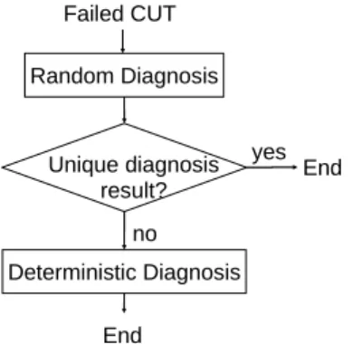
The overall CPRS diagnosis flow is shown in figure 2. The CPRS diagnosis flow can be divided into two phases: the random diagnosis and the deterministic diagnosis. The failed CUT is first diagnosed by the random diagnosis. If a unique diagnosis result is obtained after the random diagnosis, the flow is terminated. Otherwise, the failed CUT continues to the deterministic diagnosis. The random diagnosis and deterministic diagnosis are described in detail as follows.
Random Diagnosis Deterministic Diagnosis Failed CUT End End Unique diagnosis result? yes no
Paper 42.3 INTERNATIONAL TEST CONFERENCE
3
Error Matrix E4,5 E4,4 E4,3 E4,2 E4,1 E3,5 E3,4 E3,3 E3,2 E3,1 E2,5 E2,4 E2,3 E2,2 E2,1 E1,5 E1,4 E1,3 E1,2 E1,1 Selection Matrix 0 1 1 1 0 1 1 1 0 1 1 1 1 1 0 0 0 1 0 0Selected Error Matrix
0 E4,4 E4,3 E4,2 0 E3,5 E3,4 E3,3 0 E3,1 E2,5 E2,4 E2,3 E2,2 0 0 0 E1,3 0 0
Figure 4. Error Matrix, Selection Matrix, and Selected Error Matrix
2.2.1 Random Diagnosis
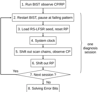
Figure 3 shows the data collection steps for the random diagnosis. Every step is explained as follows.
1. Test CUT and observe column and row parity so that the failing patterns are identified.
2. Start BIST all over again and pause after a particular failing pattern is loaded.
3. An RS-LFSR seed is loaded and the row parity register is cleared.
4. Apply one system clock.
5. Unload the scan chains. The RS-LFSR and row parity register are also clocked while unloading the scan chains. One bit of CP is observed every scan clock.
6. After unloading all scan cells, the row parity register is shifted out and observed.
7. If there are still unused RS-LFSR seeds, the procedure goes back to step 2; otherwise, the random diagnosis data collection is finished.
1. Run BIST observe CP/RP
2. Restart BIST, pause at failing pattern
3. Load RS-LFSR seed, reset RP
4. System clock
5. Shift out scan chains, observe CP
6. Shift out RP
8. Solving Error Bits 7. Next session ? No Yes one diagnosis session
Figure 3. Random diagnosis – data collection A diagnosis session consists of steps 2 to 6. Every diagnosis session has a distinct RS-LFSR seed. Note that the RS-LFSR seeds are randomly generated in advance
because no FL information is available at this time. More diagnosis sessions provide finer diagnosis results at the cost of more diagnosis time.
2.2.2 Deterministic Diagnosis
The deterministic diagnosis data collection flow is essentially the same as what is shown in Figure 3. The major difference is that the RS-LFSR seed in deterministic diagnosis is calculated based on the random diagnosis results. If one deterministic diagnosis does not produce satisfactory results, additional deterministic diagnosis can be performed iteratively. A minor difference between the deterministic and the random diagnosis is that the former does not have to determine failing patterns, which are already known after the random diagnosis.
3. Calculation
Methods
3.1 Calculate Error BitsThe failing scan chains and failing scan cells are represented by error bits in an error matrix. In the error matrix, every row corresponds to a scan chain and every element corresponds to a scan cell. A one in error bit Ei,j
means that the jth scan cell of the ith scan chain has a
mismatch between the expected good value and the actual value; a zero in Ei,j means no mismatch between the
expected good value and the actual value. Suppose the CUT has m scan chains of length l, the error matrix is of size m x l. Figure 4 shows an error matrix in which m equals to four and l equals to five.
The selection matrix is of the same size as the error matrix (m x l). A one in the selection matrix means the corresponding scan cell is selected by the row selection hardware; a zero in the selection matrix means the corresponding scan cell is masked. Figure 4 shows an example of the selection matrix of size 4 x 5. The
selected error matrix, SEM, is obtained by multiplying
the error matrix with the selection matrix. Note that the multiplication is performed in a bit-by-bit way so the SEM is also of the size m x l.
The error row parity (ERP) is a column vector of size m. The ERP represents the difference of the expected row parity and the observed row parity. A one in the xth row
Paper 42.3 INTERNATIONAL TEST CONFERENCE
4
different from its expected value. Similarly, the error
column parity (ECP) is a row vector of size l, which
represents the difference between the expected column parity and the observed column parity. The number r is the row weight of the ERP and c is the column weight of the ECP. The number r represents the total number of mismatches observed in the row parity while c represents the total number of mismatches observed in the column parity. For the Fig. 4 example, if two errors (E1,3 E3,4) are injected, the ECP and the ERP are [0 0 1 1 0] and [1 0 1 0 ]T, respectively. The weight of ECP (c) and the weight of ERP (r) are both 2. Note that, in the presence of unknown scan outputs, the corresponding ERP and ECP bits are regarded as zeros when calculating the r and c parameters. ) (ERP weight r= (1) ) (ECP weight c= (2)
The reduced SEM (RSEM) is obtained from SEM by deleting the rows for which the corresponding ERP equal to zero and deleting the columns for which the ECP equal to zero. The RSEM is therefore of size r x c. The ith row
equation is obtained by summing all elements in the ith
row of the RSEM (eq. 3). The jth column equation is
obtained by summing every element in the jth column of
the RSEM (eq. 4). A total of r row equations and a total of c column equations can be derived from a RSEM. The row equations and column equations form a system of linear equations, which can be written as Ax=B. A is called the coefficient matrix (CM). The column vector x represents all error bits to be solved and the column vector B is all ones. In the presence of unknowns, the rows and columns with unknown ERP and ECP are deleted from the SEM because they contain no information for solving the error bits.
∑
= = = c j j i RSEM i equations row 1 , 1 ) ( _ (3)∑
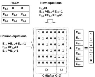
= = = r i j i RSEM j equations column 1 , 1 ) ( _ (4)Figure 5 shows an example of finding row and column equations. The first, second, and fifth columns are deleted from the SEM because the ECP is [0 0 1 1 0]. The second and fourth rows are also deleted because the ERP is [1 0 1 0 ]T. The 2 x 2 RSEM produces two row equations and two column equations. The coefficient matrix is of the size 4 x 3. Solving the system of linear equations produces a unique solution - E1,3 =1, E3,3=0, and E3,4=1 - which is the same as what we assumed earlier. This is a unique and correct diagnosis. Note that the previous row/column parity technique cannot tell a pair of errors from its diagonal counterpart because the technique does not have the row selection hardware [Sinanoglu 03]. RSEM E3,4 E3,3 0 E1,3 E1,3=1 E3,3 E3,4=1 E1,3 E3,3=1 E3,4=1 RE CE E1,3 E3,3 E3,4 1 0 0 0 1 1 1 1 0 0 0 1 1 1 1 1 * = CM
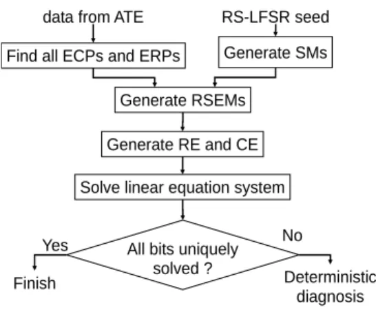
Figure 5. Derivation of Row and Column Equations The preceding example demonstrates how the error bits are solved for a particular diagnosis session. If there is more than one diagnosis session, the above process is repeated with a distinct selection matrix for each diagnosis session. A row is deleted from the SEM if no mismatch ever occurs in any session ⎯ that is, a row is included in the RSEM only if its row parity fails one or more diagnosis session. Finally, the row and column equations of different diagnosis sessions are added to the final linear equation system. Figure 6 summarizes the whole flow to solve the error bits.
Generate SMs Find all ECPs and ERPs
Generate RSEMs
Solve linear equation system
All bits uniquely solved ?
Finish Deterministic diagnosis
Yes No
Generate RE and CE data from ATE RS-LFSR seed
Figure 6. Flow to Solve Error Bits
It is not always the case that every error bit can be solved in the random diagnosis. If an error bits is uniquely solved, its diagnosis result is unique; otherwise, its diagnosis result is ambiguous. Figure 7 shows an example of ambiguous diagnosis. The number of error bits is seven but only six equations are available. After the Gauss-Jordan elimination, the CM is converted to a form of (D|U). The upper part of D is an identity matrix and the lower part of D, if any, is all zeros. If the U matrix is free of ones, a unique solution is obtained; otherwise the diagnosis result is ambiguous. In this example, only one error bit E1,3 is uniquely solved and the other error bits remain ambiguous. To diagnose the ambiguous error bits, at least one deterministic diagnosis is needed.
Paper 42.3 INTERNATIONAL TEST CONFERENCE
5
E3,4 E3,5 E3,3 E2,5 E2,4 E2,3 E1,3 1 0 0 1 0 0 0 0 1 0 0 1 0 0 0 1 1 0 0 0 0 0 0 0 1 1 0 0 0 0 1 0 0 0 0 1 0 0 0 0 0 1*
=
E3,5 E3,4 E3,3 E2,5 E2,4 E2,3 0 0 E1,3 RSEM E1,3=1 E2,3 E2,4 E2,5=1 E3,3 E3,4 E3,5=1 Row equations E1,3 E2,3 E3,3=1 E2,4 E3,4=1 E2,5 E3,5=1 Column equations 0 1 1 1 1 1 D U CM(after G-J)Figure 7. Example of ambiguous diagnosis
3.2 RS-LFSR Seed Calculation
The deterministic diagnosis is very similar to the random diagnosis except that the RS-LFSR seed of the former is calculated based on the diagnosis results of the latter. By applying a deterministic RS-LFSR seed, new row equations and column equations that are linearly independent of the existing equations are added to solve the ambiguous error bits. To find a deterministic RS-LFSR seed is equivalent to finding a desired selection
matrix (DSM), which represents the specific scan cells to
select. The DSM is of the same size (m x l) as the selection matrix. A one in DSMi,j represents that the scan
output of the jth scan cell of the ith scan chain is required to be selected; a zero represents that the corresponding scan cell is required to be masked. Figure 8 shows the flow to find a DSM. To find a DSM is similar to a covering problem. We use the following greedy algorithm to solve this problem. Note that the greedy algorithm presented here is not the only way to find the DSM; other implementations are possible.
First, the DSM is initialized to all X’s, which stand for don’t cares. (Please note that the X’s here have different meaning from the unknowns.) For all unsolved error bits Ei,j, fill in zeros in the ith row and the jth column of the DSM. A column flag (CF) vector and a row flag (RF) vector are initialized to zeros. The CF row vector is of size l and the RF column vector is of size m. A one in the CF vector indicates that the corresponding column parity is used in a column equation; a one in the RF vector indicates that the corresponding row parity is used in a row equation.
Second, find a row with the smallest non-zero weight from the U matrix and pick an unsolved error bit Ei,j from
that row. Third, check the RF vector and the CF vector of that selected error bit Ei,j. If both the CF(j) and the RF(i)
are ones, which means both the ith row parity and the jth
column parity have been used by some previous error bits, then the error bit Ei,j is marked as unsolvable in this
deterministic diagnosis. Note that an unsolvable error bit does not mean that it is unsolvable forever. It may become solvable in the future deterministic diagnosis.
1. Initialize DSM, CF, RF
2. Pick an Ei,j from U
3. RF(i) == 1 && CF(j) ==1? 4. Ei,j unsolvable 4. Ei,j solvable Set RF(i) or CF(j) Set DSMi,j=1 5. Reset column in U
6. any more ones in U? Yes End No No Yes Figure 8. Finding DSM
If the CF(j) and the RF(i) are not both ones, the error bits Ei,j is then solvable. The corresponding element DSMi,j is
set to one. Either the CF(j) or the RF(i) is flipped from zero to one. Setting the RF or the CF to one prevents the observation of the ith row parity or the jth column parity for the subsequent unsolved error bits, respectively. Fifth, reset the bits in the Ei,j column of the U matrix to zeros.
Finally, if there is still any one in the U matrix, go back to step 2; otherwise, the greedy algorithm finishes with a DSM.
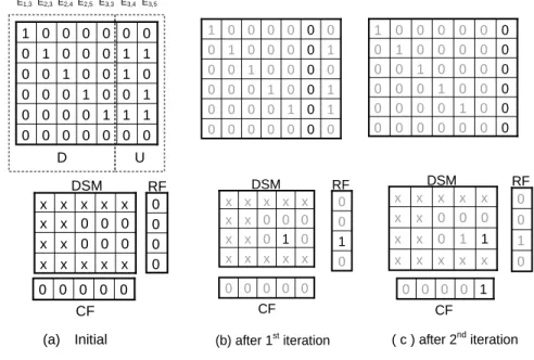
Figure 9 demonstrates an example to find DSM. Initially, all the six unsolved error bits are initialized to zero in the DSM. The error bit E3,4 is first picked because the third row of U has the smallest non-zero row weight. Since none of RF(3) and CF(4) is one, this error bit is solvable. The corresponding DSM3,4 is set to one and the RF(3) is also set to one. The whole column six in the U matrix is cleared to zeros. The second error bit picked is E3,5. Since the RF(3) is already set, the CF(5) is now set to one. The whole column seven in the U matrix is cleared. After two iterations, there is no more one in the U matrix and the final DSM is obtained.
Once the DSM is obtained, the corresponding RS-LFSR seed can be solved. Solving seeds for LFSR has been published in previous papers, such as [Koenemann 91][Al-Yamani 03], and therefore is not described here.
Paper 42.3 INTERNATIONAL TEST CONFERENCE
6
D x x x x x 0 0 0 x x 0 0 0 x x x x x x x DSM 1 0 0 1 0 0 0 0 1 0 0 1 0 0 0 1 1 0 0 0 0 0 0 0 1 1 0 0 0 0 1 0 0 0 0 1 0 0 0 0 0 1 U (a) Initial 0 0 0 0 RF 0 0 0 0 0 CF E3,4 E3,5 E3,3 E2,5 E2,4 E2,3 E1,3 DSM x x x x x 0 1 0 x x 0 0 0 x x x x x x x 1 0 0 1 0 0 0 0 0 0 0 1 0 0 0 0 0 0 0 0 0 0 0 0 1 1 0 0 0 0 1 0 0 0 0 1 0 0 0 0 0 1 0 1 0 0 RF 0 0 0 0 0 CF (b) after 1st iteration DSM x x x x x 1 1 0 x x 0 0 0 x x x x x x x 0 0 0 1 0 0 0 0 0 0 0 1 0 0 0 0 0 0 0 0 0 0 0 0 0 1 0 0 0 0 0 0 0 0 0 1 0 0 0 0 0 1 0 1 0 0 RF 1 0 0 0 0 CF ( c ) after 2nd iterationFigure 9. Example to find DSM
4. Experimental
Results
Experimental results are shown to demonstrate the effectiveness of our proposed CPRS technique. Each of the following experiment is performed on 10,000 randomly generated error matrices with various error
multiplicities. Error multiplicity is the number of ones
injected in the error matrix. The errors are assumed to be uniformly distributed in the error matrices.
4.1 Diagnosis without X
In the first experiment, a total of one thousand scan cells are partitioned into 10 scan chains (i.e., m = 10 and l = 100). Table 1 shows the average number of correctly diagnosed bits, wrong bits, and ambiguous bits. If a bit is uniquely solved, its diagnosis result is either correct or wrong, depending on whether the solution is the same as the original error matrix. If a bit is not uniquely solved, its diagnosis result is ambiguous. The numbers in table 1 are obtained from a specified number of random diagnosis sessions followed by one deterministic diagnosis session. After fifteen random diagnosis sessions and one deterministic diagnosis, every bit is correctly diagnosed even in the presence of 15 errors (1.5% of total scan cells). The same experiments are performed using the previous technique [Sinanoglu 03]. The results show that only 993 and 928 bits are correctly diagnosed for 2 and 15 errors, respectively. In comparison, the CPRS is more effective because of the random row selection mechanism.
Table 1. Diagnosis Results of 100x10 (no X)
# of random sessions
error
multiplicity correct wrong ambiguous
2 998.1 1.2 0.7 1 15 955.4 11.9 32.7 2 998.8 0.8 0.5 2 15 930.3 7.8 62.0 2 999.3 0.4 0.2 3 15 915.5 6.1 78.4 2 999.8 0.1 0.1 5 15 956.7 14.2 29.1 2 1000.0 0.0 0.0 10 15 998.8 1.1 0.1 2 1000.0 0.0 0.0 15 15 1000.0 0.0 0.0
For the 15 error cases note that the number of correctly diagnosed bits decreases by a small amount in the first few sessions. This is because the number of variables increases faster than the number of equations at the beginning of the diagnosis. This phenomenon disappears when the number of diagnosis sessions is larger than three. Table 2 shows the diagnosis results of ten thousand scan cells, which are partitioned into 10 scan chains (i.e., m = 10 and l = 1,000). The number of total bits and injected errors are ten times higher than those of the last experiment. Again, after fifteen random diagnosis sessions, all ten thousand bits are correctly diagnosed. This experiment shows that CPRS is applicable to at least ten thousand scan cells.
Paper 42.3 INTERNATIONAL TEST CONFERENCE
7
Table 2. Diagnosis Results of 1,000x10 (no X)
# of random sessions
error
multiplicity correct wrong ambiguous
20 9527.1 9.1 463.8 1 150 7673.0 108.5 2218.5 20 9540.2 10.4 449.4 2 150 7734.8 119.3 2145.9 20 9552.3 12.4 435.3 3 150 7922.6 132.5 1944.9 20 9254.3 9.6 736.2 5 150 8135.4 146.3 1718.3 20 9978.0 0.0 22.0 10 150 9940.0 0.0 60.0 20 9999.0 0.0 1.0 15 150 9999.0 0.0 1.0 20 10000.0 0.0 0.0 20 150 10000.0 0.0 0.0 4.2 Diagnosis with X
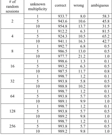
Table 3 shows the diagnosis results with fifteen errors and various unknown multiplicities, which are the number of unknowns (X’s). The locations of X’s are randomly generated, assuming a uniform distribution. The number of scan cells is one thousand, which are partitioned into 10 chains (i.e., m = 10 and l = 100), and the error multiplicity is 15. It can be seen that approximately 99% of the one thousand scan cells are correctly diagnosed, even in the presence of 10 unknowns.
One notable point in Table 3 is that, at the beginning of the diagnosis, the number of ambiguous bits for one X is more than that of ten X’s. This is because more row equations of the latter than that of the former are discarded due to the presence of more unknowns. Therefore, the number of variables involved in the former is larger than that of the latter in the first few diagnosis sessions. This phenomenon disappears when the number of diagnosis sessions is larger than eight.
Table 4 compares the percentage of correctly diagnosed bits as a function of unknown multiplicity. The numbers of CPRS are obtained from our simulations and the other numbers are obtained from [Rajski 03]. For a fair comparison, all techniques have one hundred times compression ratio (i.e. one hundred scan outputs compressed into one output). The CPRS simulations are performed on 10,000 scan cells, which are partitioned into 100 scan chains. In the presence of 1% unknowns, the CPRS correctly diagnoses all single errors and 99.8% of fifteen errors. The performance of CPRS is better than previous techniques.
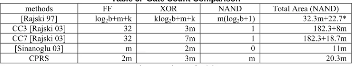
Table 5 compares the diagnosis circuitry area overhead of several techniques. The number of flip-flops, XORs, and
Table 3. Diagnosis results of 100x10 (15 errors, plus X)
# of random sessions
unknown
multiplicity correct wrong ambiguous
1 933.7 8.0 58.3 5 943.6 10.6 45.8 2 10 954.8 13.7 31.5 1 912.2 6.3 81.5 5 924.3 10.5 65.2 4 10 941.1 16.3 42.7 1 992.7 6.8 0.5 5 986.5 13.0 0.5 8 10 977.7 21.2 1.0 1 998.6 1.3 0.1 5 993.2 6.3 0.5 16 10 987.5 11.7 0.8 1 998.7 1.2 0.1 5 993.8 5.8 0.5 32 10 988.8 10.2 0.9 1 998.7 1.2 0.1 5 993.8 5.7 0.5 64 10 989.1 9.9 1.0 1 998.7 1.2 0.1 5 993.8 5.7 0.5 128 10 989.2 9.8 1.0 1 998.7 1.2 0.1 5 993.8 5.7 0.5 256 10 989.2 9.8 1.0
Table 4. Percentage of Correctly Diagnosed Bits
Technique 0.10% X 0.50% X 1.00% X XC [Mitra 02] 92.0 % 15.7 % 0.06 % CC3 [Rajski 03] 97.1 % 18.7 % 0.08 % CC7 [Rajski 03] 97.7 % 52.4 % 14.3 % CPRS – 1 error 100.0 % 100.0 % 100.0 % CPRS – 15 errors 100.0 % 99.9 % 99.8 %
AND gates are derived from the original papers. The total area is expressed in the number of equivalent NAND gates as a function of m (number of scan chains). The conversion of cell area is based on the numbers in the TSMC 0.18 µm standard cell library. The CPRS costs about 20 NAND gates per scan chain, which is approximately in the same order as the other techniques. (For the convenience of comparison, some typical numbers are assumed for [Rajski 97].)
To reduce the CPRS area overhead, the row parity can be shared with the MISR. Figure 10 shows the proposed structure of the integrated MISR/RP hardware. In diagnosis mode, the circuit is a row parity register. In BIST mode, the circuit becomes a MISR. The RS-LFSR is filled with all ones in BIST mode so all scan outputs pass through the row selection hardware without being masked.
Paper 42.3 INTERNATIONAL TEST CONFERENCE
8
Table 5. Gate Count Comparison
methods FF XOR NAND Total Area (NAND)
[Rajski 97] log2b+m+k klog2b+m+k m(log2b+1) 32.3m+22.7*
CC3 [Rajski 03] 32 3m 1 182.3+8m CC7 [Rajski 03] 32 7m 1 182.3+18.7m [Sinanoglu 03] m 2m 0 11m CPRS 2m 3m m 20.3m *assume k=m, b=16 DFF DFF DFF DFF B D B D B D B D Feedback XOR network RS-LFSR B=BIST D=Diagnosi
Figure 10. Integrated MISR/RP
5. Summary
The CPRS is an effective BIST diagnosis technique for multiple errors in multiple scan chains. The row selection LFSR randomly selects scan outputs from multiple scan chains. The column parity and row parity of the selected scan outputs are observed after every scan cycle and every scan unload, respectively. Experimental data show that CPRS correctly diagnoses all scan cells in the presence of 1% unknowns. The area overhead of CPRS is in the same order as the other techniques.
6. Acknowledgement
This research is supported by the National Science Council of Taiwan under contract number NSC 93-2220-E-002-012.
7. References
[Al-Yamani 03] A. A. Al-Yamani and E. J. McCluskey, “Seed encoding with LFSRs and cellular automata,”
IEEE Proceedings - Design Automation Conference,
p 560-565, 2003.
[Aitken 89] R. C. Aitken and V. K. Agarwal, “A diagnosis method using pseudo-random vectors without intermediate signatures,” IEEE Proceedings
- Int’l Conf. Computer-Aided Design, pp. 574-577,
1989.
[Bayraktaroglu 00] I. Bayraktaroglu and A. Orailoglu, “Deterministic partitioning techniques for fault diagnosis in scan-based BIST,” IEEE Proceedings -
International Test Conference, pp. 273-282, 2000.
[Bayraktaroglu 02] I. Bayraktaroglu and A. Orailoglu, “Cost-effective deterministic partitioning for rapid diagnosis in scan-based BIST,” IEEE Journal -
Design & Test of Computers, VOL. 19, NO. 1,
January/February, pp. 42-53, 2002.
[Chan 90] J. C. Chan and J. A. Abraham, “A study of faulty signatures using a matrix formulation, ”IEEE
Proceedings - International Test Conference,
September, pp. 553-561, 1990.
[Cheng 04] W.-T. Cheng, K.-H. Tsai, Y. Huang, N. Tamarapalli, and J. Rajski, “Compactor independent direct diagnosis,” IEEE Proceedings - Asian Test
Symposium, pp. 204-209, 2004.
[Damarla 95] T. R. Damarla, C. E. Stroud, and A. Sathaye, “Multiple error detection and identification via signature analysis”, Journal of Electronic Testing:
Theory and Applications (JETTA), VOL. 7, NO. 3,
December, pp. 193-207, 1995.
[Ghosh 99] J. Ghosh-Dastidar, D. Das, and N. A. Touba, “Fault diagnosis in scan-based BIST using both time and space information” Source: IEEE Proceedings -
International Test Conference , pp. 95-102, 1999.
[Ghosh 00] J. Ghosh-Dastidar, and N. A. Touba, “Rapid and scalable diagnosis scheme for BIST environments with a large number of scan chains”,
IEEE Proceedings - VLSI Test Symposium, pp.
79-85, 2000.
[Karpovsky 93] M. G. Karpovsky and S. M. Chaudhry, “Design of self-diagnostic boards by multiple signature analysis” IEEE Transactions on
Computers, VOL. 42, NO. 9, September, pp.
1035-1044, 1993.
[Koenemann 91] B. Koenemann, “LFSR-coded test patterns for scan designs,” Proceedings of the 2nd
European Test Conference - ETC91, pp. 237, 1991.
[Liu 03] C. Liu and K. Chakrabarty, “ Failing vector identification based on overlapping intervals of test vectors in a scan-BIST environment,” IEEE
Transactions on Computer-Aided Design of Integrated Circuits and Systems, VOL. 22, NO. 5,
May, pp. 593-604, 2003.
[McAnney 87] W.H. McAnney and J. Savir, “There is Information in Faulty Signature,” IEEE Proceedings
Paper 42.3 INTERNATIONAL TEST CONFERENCE
9
[Mitra 02] S. Mitra and K. S. Kim, “X-Compact: an efficient Response Compaction Technique for Test Cost Reduction,” Proc. IEEE Proceedings -
International Test Conference, pp.311-320, 2002.
[Mrugalski 04] G. Mrugalski, A. Pogiel, J. Rajski, J. Tyszer, C. Wang, “Fault diagnosis in designs with convolutional compactors”, IEEE Proceedings -
International Test Conference, pp. 498-507, 2004.
[Rajski 91] J. Rajski and J. Tyszer, “On the diagnostic properties of linear feedback shift registers, ” IEEE
Transactions on Computer-Aided Design of Integrated Circuits and Systems, VOL. 10, NO. 10,
October, pp. 1316-1322, 1991.
[Rajski 97] J. Rajski and J. Tyszer, "Fault diagnosis in scan-based BIST,” IEEE Proceedings -
International Test Conference, pp. 894-902, 1997.
[Rajski 99] J. Rajski and J. Tyszer, “Diagnosis of scan cells in BIST environment,” IEEE Transactions on
Computers, VOL. 48, NO. 7, July, pp. 724-731,
1999.
[Rajski 03] J. Rajski, J. Tyszer, and S. M. Reddy, “Convolutional Compaction of Test Responses,”
IEEE Proceedings - International Test Conference,
pp.745-754, 2003.
[Rajski 05] J. Rajski, J. Tyszer, S. M.Reddy, and C. Wang, “Finite memory test response compactors for embedded test applications,” IEEE Transactions On
Computer-Aided Design of Integrated Circuits and Systems, VOL. 24, NO. 4, April, pp. 622-634, 2005.
[Savir 88] J. Savir and W.H. McAnney “Identification of failing tests with cycling registers,” IEEE
Proceedings - International Test Conference, pp.
322-328, 1988.
[Savir 97] J. Savir, “Salvaging Test Windows in BIST Diagnostics,” IEEE Proceedings - VLSI Test
Symposium, pp. 416-425, 1997.
[Sinanoglu 03] O. Sinanoglu and A. Orailoglu, “Compacting Test Responses for Deeply Embedded SoC Cores,” IEEE Journal - Design & Test of
Computers, VOL. 20, NO. 4, July/August, pp. 22-30,
2003.
[Stroud 95] T. R. Damarla, W. Su, M. J. Chung, Charles E. Stroud, and Gerald T. Michael, “Built-in self test scheme for VLSI,” IEEE Proceedings - Asia and
South Pacific Design Automation Conference, ASP-DAC, pp. 217-222, 1995.
[Tekumalla 03] R. C. Tekumalla, “On Reducing Aliasing Effects and Improving Diagnosis of Logic BIST Failures,” IEEE Proceedings - International Test
Conference, pp. 737-744, 2003.
[Waicukauski 89] J. A. Waicukauski and E. Lindbloom, “Failure Diagnosis of Structured VLSI,” IEEE
Journal - Design & Test of Computers, VOL. 6, NO.
4, August, pp.49-60, 1989.
[Wohl 02] P. Wohl, J. A. Waicukauski, S. Patel, and G. Maston, “Effective diagnostics through interval unloads in a BIST environment,” IEEE Proceedings
- Design Automation Conference, pp. 249-254, 2002.
[Wohl 03] P. Wohl, J. A. Waicukauski, S. Patel, and M. B. Amin, “X-tolerant compression and application of scan-ATPG patterns in a BIST architecture,” IEEE
Proceedings - International Test Conference, pp.
727-736, 2003.
[Wu 96] Y. Wu and S. Adham, “BIST fault diagnosis in scan-based VLSI environments,” IEEE Proceedings
- International Test Conference , p 48-57, 1996.
[Wu 99] Y. Wu and S. M. I. Adham, “Scan-based BIST fault diagnosis,” IEEE Transactions On
Computer-Aided Design Of Integrated Circuits And Systems,