INVERSE FILTERING OF A LOUDSPEAKER AND ROOM ACOUSTICS USING TIME-DELAY NEURAL NETWORKS

Inverse filtering of a loudspeaker and room acoustics

using time-delay neural networks

Po-Rong Chang, C. G. Lin, and Bao-Fuh Yeh

Department of Communication Engineering, National Chiao-Tung University, Hsin-Chu, Taiwan (Received 30 July 1993; accepted for publication 28 January 1994)

This paper presents the design of a neural-based acoustic control used for the equalization of the response of a sound reproduction system. The system usually can be modeled as a composite system of a loudspeaker and an acoustic signal-transmission channel. Generally, an acoustic signal radiated inside a room is linearly distorted by wall reflections. However, in a loudspeaker, the nonlinearity in the suspension system produces a significant distortion at low frequencies and the inhomogeneity in the flux density causes a nonlinear distortion at large output signals. Both the linear and nonlinear distortions should be reduced so that high fidelity sound can be reproduced. However, the traditional adaptive equalizer which is only capable of dealing with linear systems or specific nonlinear systems cannot compensate these nonlinear distortions. The time-delay feedforward neural network (TDNN) which has the capability to learn arbitrary nonlinearity and process the temporal audio patterns are particularly recognized as the best nonlinear inverse filter of the composite system. The performance of a TDNN-based acoustic controller is verified by some simulation results.

PACS numbers: 43.60.Gk, 43.38.Ar, 43.55.Me

INTRODUCTION

The objective of the sound reproduction system has been assumed to be the "perfect" reproduction of the re- corded signals at the listener's ears, i.e., the signals re- corded at two points in the recorded space are reproduced exactly at points in the listening space. Generally, the sound reproduction system is used to achieve the perfect reproduction of the recorded audio signals at the listener's ears, i.e., the signals recorded at a point in the recording space are reproduced exactly at a point in the listening space. However, the original audio signals are imperfectly reproduced at the ears of a listener when these signals are replayed via loudspeakers in a listening room. The imper- fections in the reproduction arise from two main sources:

(i) the acoustic signals radiated inside a room are linearly distorted by wall reflections, and (ii) in a loudspeaker, the suspension nonlinearity produces a significant distortion at low frequencies and the imhomogeneity in the flux density causes a nonlinear distortion at large output signals. In order to eliminate the above two undesired factors, it is necessary to introduce inverse filters that act on the inputs to the loudspeakers used for reproduction which will com- pensate for both the loudspeaker response and the room response. Initial attempts to design such inverse filters has been considered in designing the filters used for the equal- ization of the response of the room acoustic signal-

transmission

channel.

Neely and Allen

• showed

through

computer simulations that the loudspeaker to microphone room impulse response is generally a nonminimum phase. This means that it is not possible to realize the exact in- verse of an acoustic system that has nonminimum phases.

Alternative

approachs

for the realization

of the inverse

2'3

(LSE) methods. However, this inverse is not an exact in-

verse but rather an approximate inverse of the acoustic system. The principal objective of such equalization schemes has been assumed to be the production of a "clos- est possible approximation" to the exact reproduction of a recorded audio signal at a single point in the listening space.

An account

4 of work aimed

at producing

widespread

effectiveness of the equalization of low-frequency sound reproduction in automative interiors shows that such an approach may well be useful. Since the traditional equal- ization can only deal with the linear systems or specific nonlinear systems, the suspension nonlinearity of loud- speakers will significantly degrade the quality of reproduc- tion at low frequencies by using such an equalization. For small input signals, the loudspeakers can be approximated as a linear system, and the transfer behavior is described by a linear transfer response. However, the nonlinear distor- tions, i.e., harmonics and intermodulation, increase rapidly when the input signal power becomes larger. This leads to the nonlinear inverse filters that can equalize the nonlinear distortions of the loudspeakers. Most of them are based on

the Volterra

series

expansion.

5-7

The Volterra

series

is both

efficiency.

The emerging

feedforward

neural

networks

8-•ø

have the capability to learn arbitrary nonlinearity and show great potential for nonlinear filter application. Arti- ficial neural networks are systems that use nonlinear com- putational elements to model the neural behavior of the biological nervous systems. The properties of neural net- works include: massive parallelism, high computation rates, and ease for VLSI implementation. The neural-based inverse filters would be applied to the equalization of the

Power Amplifier

r

Audio

Source

FIG. 1. A stereophonic sound reproduction system with acoustic con-

troller.

response of a composite system of both loudspeakers and

room acoustics.

I. MODEL DESCRIPTION FOR A COMPOSITE SYSTEM OF LOUDSPEAKERS AND ROOM ACOUSTICS

As alluded to earlier, the problem of loudspeaker-

room interaction draws more attention in accurate sound

reproduction. Bascially, a block diagram of a composite system consisting of loudspeakers and a room acoustic signal-transmission channel is illustrated in Fig. 1. How-

ever, a lot of researchers •-3 did not consider the nonlinear

distortion of loudspeakers which could degrade the quality of sound reproduction. In this section, we would like to review the mathematical models for the loudspeakers and

room acoustics. A nonlinear inverse filter based on time-

delay neural networks will be introduced in the next sec- tion.

A. The image models for room acoustics

Image methods are commonly used for the analysis of

the acoustic

properties

of enclosures.

Allen and Barkley

TM

Usually, a loudspeaker in a room is modeled as a point source in a rectangular cavity. A signal frequency point source of acceleration in free-space emits a pressure wave of the form,

exp[ rio(R/c--t) ]

P(co,X,X'

) =

4•rR

'

( 1

)

where P= pressure, co = angular frequency, t=time, c=speed of sound, R =distance between X and X', X=the vector that represents the loudspeaker's location (x,y,z), and X'=the vector that represents the microphone's loca- tion (x',y',z').

When a rigid wall is present, the rigid wall boundary

condition may be satisfied by placing an image symmetri- cally on the far side of the wall. Since there are generally six walls that enclose a room, the situation becomes more complicated because each image is itself imaged. Allen and

Berkley

ll showed

that the pressure

can be written,

8 • exp

[ j ((D/C)

I Rp

-Jr-

R r I ]

Z

Z

p=l r----oo

4•rlR•,+Rrl

X exp(--jcot), (2)

where

R e denotes

the eight

permutation

vectors

over the

Re= ( x + x',y + y',z + z' ) , l<p<8

Rr= 2rL = 2 ( n L• ,lLy ,m L•),

(4)

where

r-(n,l,m) is an integer

vector

and L= (Lx,Ly,Lz)

Since Eq. (2) is the pressure frequency response, its corresponding time-domain impulse response can be ob- tained by taking the inverse Fourier transform,

8 o• ti[t_(lRp_l_Rrl/c)

]

p(t,X,X')= •,

•,

.

(5)

p=l r=--oo 4•rlRp-I-Rrl

In practice, the room walls are not rigid. Allen and

Berkley

ll showed

that the nonrigid

walls

can be approxi-

mated by the above point image method with an angle- independent pressure wall reflection coefficient/3. The wall reflection coefficients are greater than 0.7 over the fre- quency range of 100 Hz4 kHz for the typical listening room geometries. Introducing the wall reflection coeffi- cients into Eq. (5), the time-domain impulse response be-

comes

1

p(t,X,X')= •

• •lxn--Pl

Inl II-71•11l•lrn---kl•

Irnl

p=O r=--oo

ti[t--( lR•,+Rrl/c) ]

X 4•riRp_l_Rrl

,

(6)

where

R e is now expressed

in terms

of the integer

vector

R e = (x -- x' + 2qx',y--y' + 2iy',z-- z' + 2kz' ).

( 7 )

R e is identical

to that of (5).

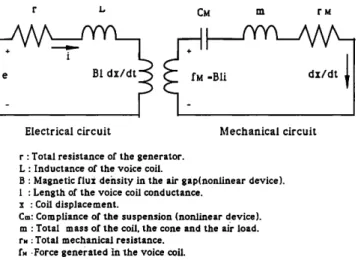
B. Equivalent electrical and mechanical circuit model for a loudspeaker

A loudspeaker is composed of an electrical part and a mechanical part. The electrical part is the voice coil. The mechanical part consists of the cone, the suspension, and the air load. The two parts interact through the magnetic field. The mechanical part can also be described by an equivalent electrical circuit. References 6 and 7 introduced an equivalent electrical circuit of a loudspeaker that is shown in Fig. 2. In the voice coil electrical circuit, e, i, r, L, and E represent the input voltage, the current in the voice coil, the electrical resistance of the voice coil, the induc- tance of the voice coil, and the voltage produced in the electrical circuit by the mechanical circuit, respectively. The voltage E is equal to Bl dx/dt, where B is the mag-

r • C• m

ß

1

e BI dx/dt =Bli

_ _

Electrical circuit Mechanical circuit

r: Total resistance of the generator.

L: Inductance of the voice coil.

B: Magnetic flux dehsity in the air gap(nonlinear device).

I : Length of the voice coil conductance.

x : Coil displacement.

C•,: Compliance of the suspension (nonlinear device).

m: Total mass of the coil. the cone and the air load.

r. :Total mechanical resistance.

f..Force generated in the voice coil.

rM

dx/dt

I

FIG. 2. Equivalent electrical and mechanical circuit of a loudspeaker.

netic flux density in the air gap, I is the length of the voice coil conductor, and x is the cone displacement. In the me- chanical circuit, rn, rM, CM, and fM denote the total mass of the coil and the air load, total mechanical resistance due to the dissipation in the air load and the suspension system, the compliance of the suspension, and the force generated in the voice coil, respectively. The force fM is equal to Bli.

Generally, the mechanomotive force in the voice coil is a nonlinear function of the displacement x. The force de- flection characteristics of the loudspeaker cone suspension system is approximated by

f M = OtX

-3-

BX

2 -3-

]/X

3.

( 8 )

Thus the compliance of the suspension system is obtained

x 1

CM--f

M--a

+ [3x

+ Tx

2 .

(9)

Another source of harmonic distortion is nonuniform

flux density B. The flux density is a function of the dis- placement x, which may also be approximated by a second- order polynomial,

B(x) = Bo+ BlX -3-

B2

x2.

Let the state variables x• =i, x2=x, and x3=dx2/dt. From the equivalent electrical and mechanical circuits, one can obtain the following state-space dynamical equation'

dx• 1

dt --L ( --rx•--

Bolx3+e--

BllX2x

3--

B21x22x3),

dt --x3'

(11)

-- ( BolXl--ax2--rMx3--lSx22--]/x•

+ lBlXlX2

+ lB2x

lx22

),

where y(t) is output signal of the loudspeaker.

(12)

II. NEURAL-BASED MODEL IDENTIFICATION

Neural networks have become a very fashionable area of research with a range of potential applications that spans artificial intelligence (AI), engineering, and science. All the applications are dependent upon training the net-

work

with illustrative

exa,,mples

and this

involves

adjusting

the weights which defin4 the strength of connection be-

tween the neurons in the network. This can often be inter-

preted as a system identification problem of estimating the system that transforms inputs into outputs given a set of examples of input-output pairs.

This section focuses on the feasibility of neural net- works and their learning algorithms for training the net- works to represent forward and inverse transform models of nonlinear acoustic systems. Training a neural network using input-output data from a nonlinear plant can be considered as a nonlinear functional approximation prob- lem. Approximation theory is a classical field of mathemat-

ics. From the well-known

Stone-Weierstrass

theorem,

•2 it

ity of networks

has

been

investigated

8-•ø

by using

the sim-

ilar concept based on the Stone-Weierstrass theorem. A number of results have been published showing that a feed- forward network of the multilayer perceptron type can ap-

proximate

arbitrarily

well a continuous

function.

8-•ø

To be

specific, these research works prove that multilayer feed- forward networks with as few as a single layer and an appropriately smooth hidden layer activation function are capable of arbitrarily accurate approximation to an arbi- trary continuous function.

Before applying the feedforward neural networks to the model identification of loudspeaker-room system, it is important to establish their approximation capabilities to some arbitrary nonlinear real-vector-valued continuous mapping y=f(x)'DC_Rn•R m from input/output data pairs {x,y}, where D is a compact set on R. Consider a feedforward network F(x,w) with x as a vector represent- ing inputs and w as a parameter-weighting vector that is updated by some learning rules. It is desired to train F(x,w) to approximate the mapping f(x) as close as pos-

sible.

The Stone-Weierstrass

theorem

12

shows

that for any

continuous

function

f•Cl(D) with respect

to x, a compact

metric space, an F(x,w) with appropriate weight vector w

can be found such that IIF(x,w ) - f(x )11 < for an arbi- trary e > 0, where Ilell is the norm defined by

Ilell-sup(lle(x)ll:xD, I1'11 is the vector norm}.

"

(13)

For network approximators, key equations are how many layers of hidden units should be used, and how many

units are required

in each layer. Cybenko

9 and Homik

ber of units. However, it is not cost effective for the

practical

implementation.

Nevertheless,

Chester

13 gave

a

Error back-propagation (Learning algorithm )

/ ... D .... /- ...

/

o

/

X•

Y -

Input layer Output layer

Hidden layers

Signal flow

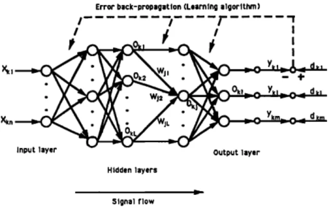
FIG. 3. Multilayer feedforward neural network.

N

E= • Ek,

(15)

where E• is the square error of the kth pattern,

1

IIm(x,w)-f(x)II 2

IIo-dll

_1 • (Okj_dkj)2

'

(16)

and N is the number

of samples,

oaj and daj are the jth

Here, we define the weighted sum of the output of the previous layer by the presentation of input pattern xa:

theoretical support to the empirical observation that net- works with two hidden layers appear to provide high ac- curacy and better generalization than a single hidden layer network, and at a lower cost (i.e., fewer total processing units). Since, in general, there is no prior knowledge about the number of hidden units needed, a common practice is to start with a large number of hidden units and then prune the network whenever possible. Additionally, Huang and

Huang

TM

gave

the lower

bounds

on the number

of hidden

A. Feedforward neural networks and their learning rules

A feedforward neural network shown in Fig. 3 is a layered network consisting of an input layer, an output layer, and at least one layer of nonlinear processing ele- ments. The nonlinear processing elements, which sum in- coming signals and generate output signals according to some predefined function, are called neurons. In this paper, the function used by nonlinear neurons is called the sig- moidal hyperbolic tangent function (7, which is similar to a smoothed step function,

(7(x) =tanh (x). (14)

The neurons are connected by terms with variable weights. The output of one neuron multiplied by a weight becomes the input of an adjacent neuron of the next layer.

In 1986, Rumelhart

et al. •5 proposed

a generalized

delta rule known as backpropagation for training layered neural networks. For control engineers, it is appropriate to

consider feedforward neural networks as a tool to solve

function approximation problems rather than pattern rec- ognition problems. In mathematical sense, the backpropa- gation learning rule is used to train the feedforward net- work F(x,w) to approximate a function f(x) from compact subset D of n-dimensional Euclidean space to a bounded subset f(D) of m-dimensional Euclidean space. Let Xk which belongs to D be the kth pattern or sample and selected randomly as the input of the neural network, let F(xk,w) (=ok) be the output of the neural network, and let f(xk)(=dk) which also belongs to f(D) be the desired output. This task is to adjust all the variable weights of the neural network such that the system error E can be reduced, where E is defined as

netkj=

• WjPki,

(17)

i

where

wji is the weight

that connects

the output

of the ith

neuron in the previous layer with respect to the jth neu- ron, and oki is the output of the ith neuron. It should be noted that oki is equal to xki when the ith neuron is located in the input layer, where xki is the ith component of pattern x k. Using (14), the output of neuron j is

xkj, if the neuron

j belongs

to the input layer

(7(net•), otherwise.

(18)

As discussed above, the goal is to choose the network

connection

weights

Wji'S

such

that the system

error E is

the backpropagation

algorithm.

•6 The algorithm

computes

iteratively the partial derivatives of the system error E with respect to each parameter and modify the parameter in order to achieve a gradient descent in E with a momentum term added to dampen oscillations. In particular, the

weight

Wji is updated

at the t+ 1st

iteration,

according

the

rule,

c•E

Awji(t+

1)=--(

1--a)r/(t+

1)

•-•ji+aAwj•(t),

(19)

where

Awji(t-[-1) is the weight

increment

for the t+ 1st

iteration, r/(t + 1 ) is the learning rate value corresponding to Aw(t+ 1 ) at time t+ 1, and a is the momentum rate.

Since

the expression

of OE/Owij

could

be in terms

of

OEk/Owij's,

it is useful

to see this partial derivative

for

pattern

k, OEk/OWii

, as resulting

from the product

of two

c•Ek c9Ek c9

netkj

• o

C•Wji • netkj c•wji

From (17), the second part becomes

(20)

•WJ

i __•Wji

. WjtOki

=Oki.

(21)

An error signal term 6 called delta produced by the jth

neuron is defined as follows:

0Ek

8•-• 0(net•j)

'

(22)

Note that E is a composite

function

of netkj, it can be

=E•(G(net•l ),G(net•2) .... ,G(net•L)), (23) where L is the number of the neurons in the current layer. Thus we have from (22),

0Ek 0o•j

ß (24)

•kJ=

-0o•,j

a netkj

Denoting the second term in (24) as a derivative of the

activation function,

aOk]

-- G' (net•j).

(25)

a net•

However, to compute the first term, there are two cases. For the hidden-to-output connections, it follows the definition of Ek that

OEk

OOk•

.= -- ( dkj--Okj

) .

(26)

Substituting for the two terms in (24), we can get

t•kj: ( dkj --Okj

) G' ( netkj

) .

( 27 )

chain rule is used to write

aEk aEk a netk/

Ook•--

• O

netk/

Ook-•-.

----

Z 8klWlj.

Substituting into (24), it yields

(28)

8kj

= G' (netkj)

• 8kzWtj.

( 29

)

Equations (27) and (29) give a recursive procedure for computing the 8's for all neurons in the network. Once those error signal terms have been determined, the partial derivatives for the system error can be computed directly by

N N N

0E

_{-- awji- a netkj}

0Ek

0Ek

a netkj

_awji

_{-- -- • •kjOki'}

aw/i k= 1

k= 1

k= l

(30a) where

•kj:

(dkj--okj)6' (netkj),

if neuron j belongs to the output layer,

G'

(netkj)

• 8k•w/i,

otherwise.

(30b)

It should be mentioned that oki is equal to xki when neuron i belongs to the input layer. The expression of Eqs. (30a) and (30b) is also called the generalized delta learning rule.

Jacobs 16 showed that the momentum can cause the weight to be adjusted up the slope of the system error surface. This would decrease the performance of the learn-

ing algorithm.

To overcome

this difficulty,

Jacobs

16

pro-

posed a promising weight update algorithm based on the delta-bar-delta rule which consists of both a weight update rule and learning rate update rule. The weight update rule is the same as the steepest descent algorithm and is given by (19). The delta-bar-delta learning rate update rule is

described as follows: Ar/(t+ 1) = where OE

•(t)--Owij

it(t) = ( 1 -- 0)it (t) +0it(t-- 1 ). (3 lc) In these equations, it (t) is the partial derivative of the

system

error with respect

wij at the tth iteration

and it (t)

B. Forward and inverse system model identification by feedforward network

In gereral, system identification is usually recognized as a process to train networks to represent nonlinear dy- namical systems and their inverses. This would be dis- tinctly helpful in achieving the desired output signal of the system. The issue of identification is perhaps of even greater importance in the field of adaptive control and sig-

nal processing

systems.

17 Since

the plant in an adaptive

control varies in operation with time, the adaptive control must be adjusted to account for the plant variations.

The procedure of training a neural network to repre- sent the forward dynamics will be referred to as forward

model

identification.

The basic

configuration

f6r achieving

Loudspeaker and Room acoustics ! I I I I I I 0 _ I I I I

•III

II II II••

r

...

• y

FIG. 4. Forward model identification.

with the system and receives the same input x as the sys- tem. The system output provides the desired response d during training. The purpose of the identification is to find

the appropriate

weights

w•js

of the network

with response

o that matchs the response y of the system for a given set of inputs x. During the identification, the norm of the error

vector, Ilell--Ila--oll, is minimized through a number of

weight adjustments by the delta-bar-delta learning rule. In our case, those weights are updated by minimizing the

system

error,

E=

by the

same

algorithm,

where

ek= (dk--Ok). Figure 4 shows the case for which the net- work attempts to model the mapping of system input to output, which both input and output measured at the same time. With sufficiently large number of hidden units,

Stone-Weierstrass theorem shows that the neural network

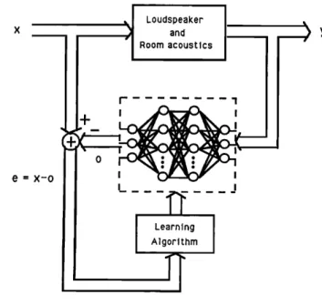
will be identical to the system in the domain of interest. Figure 4 shows use of a feedforward neural network for direct modeling of an unknown system to obtain a close approximation to its responses. By changing the configu- ration, it is possible to use the feedforward network for inverse modeling to obtain the reciprocal of the unknown system's transfer function when the system is invertible. In contrast to forward system characteristics identification, the system output o is used as neural network input, as shown in Fig. 5. The unknown system's input x delayed by A time units is the desired response of the feedforward network. Thus the error vector of network training is com-

puted as a x(t--A)-o(t). The system erro_r to be mini-

mized through learning

is therefore

E=•_•llx(tk

--A)--o(t•) II

2. The neural

network

trained

by the delta-

bar-delta algorithm will implement the mapping of the sys- tem inverse. Once the network has been successfully trained to mimic the delayed system inverse, it can be used directly for inverse feedforward control. In other words,

the inverse model is cascaded with the controlled unknown

system in order that the composed system results in an identity mapping with a time delay A between desired re- sponse (i.e., the network inputs) and the controlled system

FIG. 5. Inverse model identification.

output. The output of the system follows the input signal delayed by A time samples.

As mentioned, it is assumed that the system is invert- ible. Then there exists an injective mapping which repre- sents its inverse. If it is not true, a major problem with system inverse identification arises when the system inverse is not uniquely defined. A second approach to inverse mod- eling which aims to overcome these problems is known as

specialized

inverse

learning.

•8 As pointed

out in Psaltis

et al., 18

the specialized

method

allows

the training

of the

inverse network in a region in the expected operational range of the system. On the other hand, the generalized training procedure produces an inverse over the operating space which may be uniquely defined. Fortunately, the mapping of a loudspeaker-room system may have a unique inverse or its approximation. Thus we could apply the di- rect invesre method as illustrated in Fig. 5 to find the approximation of the inverse. In addition, since the non- linearity of a system inverse is higher than that of forward modeling, a network with two hidden layers is considered in constructing the inverse modeling.

III. INVERSE FILTERING AND MODEL IDENTIFICATION OF A LOUDSPEAKER-ROOM SYSTEM BY THE TIME DELAY NEURAL NETWORK

As discussed in the above section, the feedforward neural network results in a static network which maps static input patterns to static output patterns. Any tempo- ral patterns in the input data are not recognizable by such a network. A time delay neural network (TDNN) shown in Fig. 6 is extended to networks with delay elements in the connections can be trained to recognize specific spectral

structures

within a consecutive

frame

of audio signal.

•9

Usually, these temporal audio patterns generated by loudspeaker-room system can be governed by a nonlinear discrete-time difference equation where the output has a finite temporal dependence on the input, that is,

I ul(k)

I u2(k)

Mullilaver Perceotron

x(k)

J

-•[ Tapped

Delay

Line

y(t) =f{x(t--A f),x(t--A f-- 1 ),...,x(t--A f--nf)),

(32)

where

Af is the forward

system

time delay

and (A f+ n f) is

This architecture is equivalent to a linear finite impulse response (FIR) filter when the function f( ß ) is a weighted

linear sum. This would be identical to our method without

including the nonlinearity of the loudspeakers. The trans- fer function of the acoustic signal-transmission channel be- tween loudspeaker and microphone is denoted as G(z), which is a FIR (finite impulse response) system, G(z) represents the reflective sound as well as the direct sound between the loudspeaker and microphone.

To process the time series data generated by (32), it is possible to convert the temporal audio sequence into a static pattern by unfolding the sequence over time and then use this pattern to train a static network. From a practical point of view, it is suggested to unfold the sequence over a finite period of time. This can accomplished by feeding the input sequence into a tapped delay line of finite extent, then feeding the taps from the delay line into a static feedfor-

ward network. Because there is no feedback in this net-

work, it can be trained using the standard backpropagation algorithm.

Since the input-output structure of a real acoustic sys- tem involves the loudspeaker's nonlinearity, it is quite dif- ficult to describe clearly the dynamic behavior of the in- verse of a nonlinear system. For simplicity, we would like to discuss the linear acoustic signal-transmission channel and its inverse. Generally, Refs. 1 and 2 showed that the transfer function of the acoustic channel G(z) is consid- ered to be a nonminimum phase system where G(z) has

one or more of its zeros outside the unit circle in the z

plane. A reciprocal transfer function D(z){=l/G(z)} would then have unstable poles. Usually, the reciprocal function D(z) can be decomposed into two component subsystems, each of which has all of its poles either inside or outside the unit circle, that is,

D(z)=D½(z)Dac(Z), (33)

where De(z) and Dac(Z) have stable and unstable poles, respectively.

In other words, the system implements D(z) by a cas- cade connection of the subsystems De(z) and Dac(Z). Be- cause the poles of De(z) are inside the unit circle, a stable causal recursive filter can implement De(z). Since the poles of Dac(Z) are outside the unit circle, no stable implemen- tation of Da½(Z) exist if the causality is required. However, by allowing their impulse responses to extend backward in time, the stable inverse filter does exist. To better under- stand this principle, it is necessary to review the properties of the bilateral z transform. A specific pole contributes either to the causal or the anticausal portion of the impulse response of Da½(Z) depending on the associated region of convergence (ROC) of its z transform. Consider a circle in the z plane that is centered at the origin and that passes a pole; if the Roe associated with the pole lies outside that circle, then the time response extends forward in time. Conversely, if the ROC of the pole is inside that circle, the time response extends backward in time. For example, the same expression of Dac (z) = z/z-- a, a > 1 yield two differ- ent impulse responses, that is, a stable anticausal impulse

response h •[n] = - (a) nu[- n- 1] and an unstable causal impulse response h2[n ] = (a)nu[n], where u[n] is a discrete-

time unit step function.

The Roe of the entire system is the intersection of the ROes of all the poles. This intersection must include the unit circle for the system to be stable. Therefore, there exists a stable inverse to G(z) when the impulse response of Dc[z ] is strictly causal and the impulse response of Dac(Z) is strictly anticausal. If the anticausal impulse re- sponse is finite in duration, noncausal filtering can be achieved exactly when the filtering introduces delay, effec- tively shifting the impulse response until it is strictly

causal.

Moreover,

Widrow

17 showed

that the anticausal

u( t) =g{x( t-- A/),x( t-- A/-- 1 ) ,...,x( t-- A/-- n•) ),

(34)

where x (t) is the input voltage, u (t) is the driver voltage to the loudspeaker, A• is the system inverse time delay, and (A•+ n•) is the maximum lag in the input.

Similarly, the TDNN can implement the nonlinear FIR filter by inputting the temporal audio signal, i.e., x(t) to a tapped delay line, then feeding the taps from the delay line into a static feedfoward network. Next the output of the static network, i.e., u(t) acts as a drive voltage to the composite system of loudspeaker and room acoustic chan- nel. From the previous section, the inverse of the compos- ite system can be identified by minimizing the system error

E-•,•-•llx(t•-%)-O(t•) II

2 where

O(tk) is the

kth sam-

ple of the response of the composite system. The trained

x(n)

Time Delay Neural Network

FIG. 7. TDNN-based plant inverse acoustic controller.

1 0.8

y(•.•

0.6

TDNN-based inverse model can be cascaded with the com-

posite system and then preequalize its response. The prop- erly trained TDNN acts as the inverse feedforward con- troller in the configuration as illustrated in Fig. 7.

IV. ILLUSTRATED EXAMPLES

To evaluate the performance of TDNN-based model identification, the simulation of the composite system of loudspeakers and room acoustics is performed by a fourth- order Runge-Kutta method with sampling period= 1/5

kHz= 2 X 10-4s.

The dimensions

of the rectangular

listen-

ing room are 10X 15X 12.5 ft 3 with equal

wall reflection

coefficients

of/3x=/Jy=0.9 and with floor and ceiling

re-

pulse

response

can

be calculated

using

the image

method.

TM

For the simulation of loudspeakers, it requires knowing the values of the associated parameters, that is, (r/L)=l.1, ( Bol/L ) =0.2, ( Bol/rn ) =0.6, (a/m) =0.5, ( rM/rn ) =1.15, (B11/L)=O.04, (B21/L)=O.05, (r/m)=O.08, (lB1/m) --0.01, and (lB2/m) =0.02 which are suggested by Ref. 6. Since/3 is very small in practice,/3 is chosen as zero. Notice that e of (11) is the input voltage to the dynamic system. Here, y(t) of (12) is the resulting output of the loudspeaker and also acts as an input signal to the room acoustic signal transmission channel. As a result, the

0.8 0.6 0.4 0.2 -0.2 -0.4: -0.6 '0'80 50 100 150 200 250 300 350 sample point 't60 150 200 250 300 350 400 ;00 sample point

FIG. 9. Comparison of the desired response (--), the response without equalizer (.--), and the response (---) with TDNN-based equalization.

response of a composite system of loudspeaker and room acoustics is produced by convolving y(t) with the calcu- lated room impulse response.

Two TDNNs with one hidden layer and two hidden layers are designed to learn the forward and inverse models of the composite system, respectively. According to Huang

and Huang's

suggestions,

TM

it is possible

to estimate

the

are chosen as 30 for each layer. For the TDNN associated

with the forward

model,

the number

of taps

and Af deter-

mined

by the model

validation

test

2ø

are equal

to 100 and

40 units, respectively. Similarly, the tap number and As of

the TDNN for the inverse model are chosen as 100 and 90

units, respectively. By inputting 10 000 random sequence with unity maximum amplitude into the composite system and then performing the delta-bar-delta algorithm on the TDNN-based forward model, the training root-mean- square error (rms) can be found as 0.0031. Similarly, it can be found that the training error is 0.007 for TDNN-

based inverse model.

Next, we would like to verify the performance of both the estimated TDNN-based forward and inverse models by a test signal x(t) =0.3 sin(1.28wt) +0.5 cos(3.93wt), where co= 200rr. The resulting error for the TDNN-based forward and inverse model are 0.015 and 0.0267, respec- tively. Figure 8 illustrates a comparison of the responses of both the composite system and TDNN-based forward model. Figure 9 shows the tracking performance of the TDNN-based inverse feedforward control. The presented curves clearly show the performance improvement that is achieved by using the proposed inverse model. It should be noted that the error resulted from the composition system without including the TDNN-based inverse controller

would become 0.2951. The TDNN-based inverse controller

improves the performance of the sound reproduction by an order of magnitude.

v. CONCLUSION

FIG. 8. Comparison of the desired response (--) from the actual system and the response (---) from the estimated forward model.

The use of TDNN-based inverse filters for loud-

speaker-room correction promises to bring a new level of

accuracy to sound reproduction systems. The inverse filter is simply cascaded with the controlled system in order that the composed system results in an identity mapping be- tween desired response (i.e., the network inputs) and the controlled output. A model of combining the room acous- tics and loudspeaker's system dynamics has been devel- oped and studied which take into account a linear rever- berant distortion and two principal sources of nonlinear loudspeaker distortion. Based on this, simulations of the proposed method have been performed. The results have

shown that both linear and nonlinear distortions of the

composite system can be reduced by an order of magni- tude.

ACKNOWLEDGMENT

This work was supported by the National Science

Council, Taiwan, under Contract NSC 81-0404-E-009-027. S. T. Neely and J. B. Allen, "Invertibility of a room impulse response," J. Acoust. Soc. Am. 66, 165-169 (1979).

Masato Miyoshi and Yutaka Kaneda "Inverse filtering of room acous- tic," IEEE Trans. Acoust. Spee6h Signal Process. 36, 145-152 (1988). p. A. Nelson, H. Hamada, and S. J. Elliott, "Adaptive inverse filters for

stereophonic sound reproduction," IEEE Trans. Acoust. Speech Signal

Process. 40, 1621-1632 (1992).

4S. J. Elliott and P. A. Nelson, "Multiple point least squares equalization

in a room using adaptive digital filters," J. Audio Eng. Soc. 37, 899-907

(1988).

5R. L. Greiner and M. Schoessow, "Electronic equalization of closed-

box loudspeakers," J. Audio Eng. Soc. 31, 125-134 (1980).

6F. X. Y. Gao and W. M. Snelgrove, "Adaptive linearization of a loud-

speaker," IEEE Int. Symp. Circ. Syst. 3589-3592 (1991).

? A. J. M. Kaizer, "Modeling of the nonlinear response of electrodynamic

louspeaker by a Volterra series expansion," J. Audio Eng. Soc. 35,

421-433 (1987).

8K. Hornik, M. Stinchcombe, and H. White, "Multilayer feedforward

networks are universal approximators," Neural Networks 2, 359-366

(1989).

9 G. Cybenko, "Approximations by superposition of a sigmoidal func-

tion," Math. Control Syst. Signals 2, 303-314 (1989).

•øK. Hornik, M. Stinchcombe, and H. White, "Universal approximation

of an unknown mapping and its derivatives using multilayer feedfor-

ward networks," Neural Networks 3, 551-560 (1990).

• J. B. Allen and D. A. Berkley, "Image method for efficiently simulating small-room acoustics," J. Acoust. Soc. Am. 65, 943-950 (1979). •2M. E. Cotter, "The Stone-Weierstrass theorem and its applications to

neural nets," IEEE Trans. Neural Networks, 1, 290-295 (1990). 139. Chester, "Why two hidden layers are better than one," in Proceed-

ings of the International Joint Conference on Neural Networks (IEEE, Washington, DC, 1989), pp. 613-618.

•4S. C. Huang and Y. F. Huang, "Bounds on the number of hidden

neurons in multilayer perceptrons," IEEE Trans. Neural Networks, 2,

47-55 (1991).

15D. E. Rumelhart, G. E. Hinton, and R. J. Williams, "Learning internal

representations by error propagation," in Parallel Distributed Process- ing, edited by D. E. Rumelhart and J. L. McCelland (M.I.T., Cam- bridge, MA, 1986), pp. 318-362.

16R. A. Jacobs, "Increased rates of convergence through learning rate

adaptation," Neural Networks, 295-307 (1988).

17 B. Widrow and R. Winter, "Neural nets for adaptive filtering and adap-

tive pattern recognition," IEEE Comput. Mag. 21, 25-39 (1988).

•SD. Psaltis, A. Sideris, and A. A. Yamamura, "A multilayer neural

network controller," IEEE Control Syst. Mag. 8, 17-21 (1988).

19A. Waibel, T. Hanazawa, G. Hinton, K. Shikano, and K. J. Lang,

"Phoneme recognition using time-delay neural networks," IEEE Trans. Acoustic Speech Signal Process. ASSP-37, 328-339 (1988).

2øS. A. Billings and W. S. F. Voon, "Correlation based model validity tests for non-linear models," Int. J. Control 44, 235-244 (1986).