FINITE MATRIX COMPUTATIONS APPLIED TO THE SCATTERING OF A WAVEPACKET IN THE COULOMB POTENTIAL

This content has been downloaded from IOPscience. Please scroll down to see the full text.

Download details:

IP Address: 140.113.38.11

This content was downloaded on 28/04/2014 at 15:52

Please note that terms and conditions apply.

Finite matrix computations applied to the scattering of a wavepacket in the Coulomb potential

View the table of contents for this issue, or go to the journal homepage for more 1995 J. Phys. B: At. Mol. Opt. Phys. 28 L69

(http://iopscience.iop.org/0953-4075/28/4/001)

1. Phys. 8 : At. Mol. Opt. Phys. 28 (1995) L69-L75. Printed in the UK

LETTER TO THE EDITOR

Finite matrix computations applied to the scattering

of

a

wavepacket in the Coulomb potential

Ue-Li Pent and T F Jiangt

t Department of Astrophysical Sciences, Princeton University, Princeton. NJ 08544-100, USA

t Institute of Physics, National Chiao Tung University, Hsinchu, Taiwan 30050, Republic of

China

Received 22 November 1994

Abstract. We develop a finite dimensional matrix method to m a t wavepacket propagation in potential scattering problems ?be method is useful for general quanNm mechanical problems. The scattering dynamics of a minimum unceminty wavepwket in the Coulomb potential is presented.

In this letter, we propose to approximate a physical problem through finite dimensional matrix representation of observables. An implementation of this method to the above- threshold-ionizaton of atomic hydrogen has been published (pen and Jiang 1991). We present here a study of tbe scattering of a minimum uncertainty wavepacket in the Coulombic potential.

Coulombic potential scattering is one of the paradigms in the development of quantum mechanics. Both quantum theory and classical mechanics lead to the correct Rutherford cross section formula. However, the quantum Rutherford formula is obtained with plane wave incidence and usually treated in a time-independent way. It is of interest to represent the incident particle by a wavepacket and

to have

a picture of the time evolution of the system. Unfortunately this type of calculation is not easy (Sakurai 1985). There are several works on the scattering of a wavepacket by a step potential (Goldberg etal 1967, Diu 1980, Brandt and Dahmen 1990) but it is difficult to find a wavepacket treatment of Coulomb scattering. However, the dynamics of a wavepacket is of fundamental importance. We h o w that even the motion of a minimum uncertainty wavepacket under no external force has interesting dynamics (Schiff 1971).

The Coulombic singularity at the origin and the long-range interaction nature of the problem sometimes cause previously effective numerical procedures from the study

of

related problems to fail. For instance, in atom-laser interaction problems, a softened Coulomb potential has been used to avoid singularity at times (Eberly eta1 1989, Javanainen

etal 1988, Rae and Burnett 1993, Rae etal 1994). Indeed the form of the softened potential affects ionization (Grochmalicki et al 1991, Mknis er al 1992). Furthermore, the spatial spread of a wavepacket as time evolves usually demands a large grid which strains the capacity of even modest current high-speed computers. The following two choices allow us to break through the limits: (i) the use of the Heisenberg picture, where we only require the space grids to represent the initial state, with no need for an increasing spatial range due to wave propagation as time goes on; and (ii) the use of a finite dimensional matrix representation for the observables. As an illustration, we choose the harmonic oscillator 0953-4075~5M40069+07$19.50 @ 1995 IOP Publishing Ltd

L69

L70 Letter to the

Editor

eigenstates as

a

basis. This forms a complete L2 set

so

that any bound or continuum state can be expanded in this basis.

We study in this IeUer the scattering of a wavepacket i n the one-dimensional Coulomb potential. This formalism

can

be straightforwardly generalized to other problems. We describe our approach below. Consider

We require as a boundary condition that all solutions vanish for x -+ 0. So the basis set used contains the odd eigenfunctions of the simple harmonic oscillator:

The well-known normalized odd eigenfunctions in coordinate representation are:

4;

= N ( H , ( C U X ) exp(-w2x2/2) (3)

E( = (i

+

$)w0

i = 2 n + 1 n = 0 . 1 , 2 , 3

,...

where a4 = mk, 00 =

Jk7;;;.

H ; ( x ) ~ i s the Hermite polynomial and atomic units are used throughout. For Hamiltonian ( I ) , the Heisenberg state

IQH)

i s independent of time and related to the Schrodinger state IW,) through a unitary transformation U ( t ) :

u(t) = e-iHsr. (7)

The observable

6"

in the Heisenberg picture is related to the Schrodinger observable

6s

by

&

= Ut6SrJ. ( 8 )

H

= SASt

(9)

If we diagonalize the Hamiltonian matrix by a similarity transformation S:

then

(10) Since our basis functions are not eigenfunctions of the Hamiltonian ( I ) , its matrix elements are not diagonal and we have to compute them explicitly. The matrix elements of I j x and x are not easy to handle in the harmonic oscillator basis. Consider

Leffer to the

Edifor

L71

as an example, although by expanding the Hermite polynomials i n algebraic form, the integrals can be found term by term in standard integral tables (Abramowitz and Stegun 1972), the large values of the coefficients of high-power terms lead to cancellation errors. The numerical results fail to be meaningful for i, j

2

IS in double precision.

A way out of the problem is to apply the finite matrix idea. In practical calculations, we are always working with a finite basis set, so we consider the following sum in a finite dimensional vector space:

This is clearly not an identity matrix as would be expected in an infinite dimensional Hilbert space. Since the numerical calculation must he carried in finite dimensional space, and we have to be consistent with the relation @irac 1926)

(14)

^ ^

xx =

2

as

well as for

m e

of calculation, we define the finite dimensional matrix elements by

Here Axx is the diagonalized matrix of xi. These definitions force the second term in equation (13) to vanish identically. The various position observable functionals (such as .?,i', .?-I,.

.

.) share common eigenstates. We then choose the most easily computed

position observable and obtain the matrix representations of its derived observables in the same way

as

equation (16). For example, from equation (2) we can find easily the matrix elements: (4i

-

1)/2 J-/2 for i = j f o r i = j - I otherwise.

With this result, other functionals of observable i can be calculated along the same lines

as

equations (15) and (16). In this way, the Coulomb potential I/x turns out to be a matrix operator. The singularity is regularized naturally.

For the calibration of our calculation, we study the propagation of an eigenstate of Hamiltonian (1). In figure 1, we show the variation of the second excited state with respect to both space and time. The calculation is carried out as follows.

L72

Proboblily 1 .o 0.5 0.0 0.0

Leffer

to the

Editor

0

Figure 1. Change of probabilily density with respect to coordinate and lime, This is for lhe second

excited state. The probability is in relative s d e .

where

I@;)

is the basis function

of

equation (2) and e& is calculated in the finite dimensional harmonic oscillator basis and diagonalized as in equation (10). The probability density I(xlIv&))12 is stationary as it should be. The size of the basis set used in the calculation is n = 30. These calculations show the reliability of our approach. Also in the above calculation, the only time dependence is in the factor e-iAr. This enables us to calculate the wavefunction at any global time in one step without propagating the wavefunction step by step in time like popular finite difference algorithms. We regard this

as

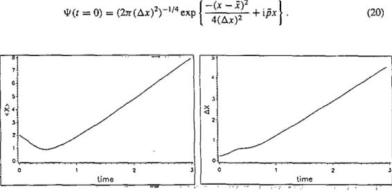
a very useful starting point for time-dependent calculations. Transformations between different pictures can also be accomplished easily.

Now consider the problem of Coulomb scattering. The Coulomb scattering problem is a good test case in the development of numerical methods. As we have stated, the singularity at the origin is crucial to many numerical methods. We consider an incoming minimum uncertainty wavepacket with i = 2, Ax = 1/4, ,5 = -2 and

Figure 2 Average position against lime. Figure 3. Position uncertainty against time,

In figure 2 we show the change in average position with time. The wavepacket is attracted toward the singularity first by the Coulomb force and bounces backward around

Letter to

the

Editor

L73

I

-

J

I

0 time 1.9 , 0 2

Figure 4. Average momentum against time. Figure 5. Momentum uncetrainty against time.

t = 0.5. Figure 3 is the corresponding change in position uncertainty, There is small bump around t = 0.5 and then Ax increases linearly in time. Figure 4 shows the time history of the momentum average. The initial momentum

p

= -2 of the wavepacket is unchanged until it enters the scattering region around t = 0.5 where the momentum reverses gradually and keeps around

p

= +2 afterwards. The momentum uncertainty remains unchanged beyond

the Coulomb-interaction dominant region as shown in figure 5. This is quite reasonable: away from the Coulomb centre, there is no obstacle to change the momentum and hence ii and A p are roughly unchanged. The position variables

i,

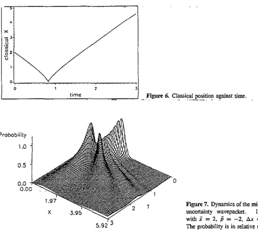
Ax increase in the way described in standard reference books (Schiff 1971). Since A x increases approximately linearly in time and A p is constant, the product is obviously linear in time. This means the coherence is soon lost in this problem, in contrast to the harmonic oscillator potential, where coherence is always maintained (Walker and Preston 1977). In the classical counterpart, the particle with initial condition x = 2 , p = -2 will impact on the Coulomb centre at f = t~ = 0.8264 and reflect back. The trajectory is described hy

and subjected to the energy constraint

In figure 6 we plot the classical position as a function of time. The conservation of total energy keeps the system from collapse to the attractive centre. The correspondence between quantum and classical behaviour can be found by comparing figures 2 and 6. Finally, a three-dimensional graph (figure 7) shows the evolution of the relative probability density in space and time. This picture shows the scattering dynamics clearly. I n the calculation the algorithm used is equation (19) and a basis set n = 100 was used to obtain convergent results. Since matrix operations are fully vectorizable, computations with IZ = 1000 and higher are

easily accomplished on a vector machine. Much smaller values of n are satisfactoly as the convergence is rapid.

In'summary, using the definition of finite matrix elements as in equations (15) and (16), the singularity can be removed reasonably. The Heisenberg representation enables us to

L74

Letter to the Editor

~~ ~

Figure 6. C l y i c a l position apinst time.

,.., .

.

.,..,.,,, ,.,., , Probobiiity 1 .o 0.5 0 0.0 0.0

Figure 7. Dynamics of the minimum uncertainty wavepacket. Initially wifi 2 = 2, f = -2, A A = 114. The probability is in relative scale.

calculate the dynamics globally in time, There will be much potential benefit in dynamics calculations for time-dependent problems. The harmonic oscillator basis is used only to demonstrate our ideas. Our method can be applied to other bases as well. A comparison between conventional coordinate and momentum representation as well

as

Sturmian and Hermite bases have been investigated and will be presented shortly.

This work was supported by the National Science Council

of

Taiwan under the contract of number NSC-84-2112-M009-002.

References

Abmowitz M and Stegun I A 1972 Hmdboouk ofMaIhemiCol Funclions (New York: Dover) Brandt S and Dahmen H D 1990 Quantum M ~ c h ~ i c s on the Personal Computer (Berlin: Springer) p 55

Dirac P A M 1926 Pmc. R. Soc. A 109 642

Diu B 1980 Eur. J. Phys. 1231

Eberly 1 H, Su Q and Javanainen 1 1989 P h y . Rev. Lett. 62 881

Goldberg A, Sehey H M and Schwvtr 1 L 1967 Am. J. Phys. 35 177

Grochmalicki, Lewenntein M, and RwLewslti K 1991 Phys. Rev. Let[. 66 1038

Javanainen J, Eberly J H and Su Q 1988 Phys. Rev. A 38 3430

Menis T, Taieb R, WNard and Maquet A 1992 J. Phys. E: At. Mol. OpI. Phys. 25 L263

Pen Ue-Li and limg T F 1991 Phys. Rev. A 46 4297

Rae S C and Burnen K 1993 Phys. Rev. A 48~2490 Rae S C. Chen and Bumett K 1994 Phys. Rev. A 50 1946

Letter

to

the

Editor

Sakurai I I 1985 Modern Quanru,n Merhunics (Taipei: BenjaminlCummings) p 386

Schiff L 1 1971 Qwrnrum Mechanics 3rd edn. Section 12 (New Yo* McCraw-Hill) Schriidinger E 1926 Ann. Phys. 79 361

Waker R Band Preston R K 1977 J. Chem Phys. 67 2017