This article was downloaded by: [National Chiao Tung University 國立交通大學] On: 27 April 2014, At: 23:13
Publisher: Taylor & Francis
Informa Ltd Registered in England and Wales Registered Number: 1072954 Registered office: Mortimer House, 37-41 Mortimer Street, London W1T 3JH, UK
The American Statistician
Publication details, including instructions for authors and subscription information:
http://www.tandfonline.com/loi/utas20
The Inequality Between the Coefficient of
Determination and the Sum of Squared Simple
Correlation Coefficients
Gwowen Shieha
a
Gwowen Shieh is Associate Professor, Department of Management Science, National Chiao Tung University, 1001 Ta Hsueh Road, Hsinchu, Taiwan 30050, Republic of China . This work was partially supported by National Science Council of Taiwan under contract number NSC89-2118-M-009-016. The author thanks the associate editor and referees for helpful comments that improved the presentation of this article.
Published online: 01 Jan 2012.
To cite this article: Gwowen Shieh (2001) The Inequality Between the Coefficient of Determination
and the Sum of Squared Simple Correlation Coefficients, The American Statistician, 55:2, 121-124, DOI: 10.1198/000313001750358437
To link to this article: http://dx.doi.org/10.1198/000313001750358437
PLEASE SCROLL DOWN FOR ARTICLE
Taylor & Francis makes every effort to ensure the accuracy of all the information (the “Content”) contained in the publications on our platform. However, Taylor & Francis, our agents, and our licensors make no representations or warranties whatsoever as to the accuracy, completeness, or suitability for any purpose of the Content. Any opinions and views expressed in this publication are the opinions and views of the authors, and are not the views of or endorsed by Taylor & Francis. The accuracy of the Content should not be relied upon and should be independently verified with primary sources of information. Taylor and Francis shall not be liable for any losses, actions, claims, proceedings, demands, costs, expenses, damages, and other liabilities whatsoever or howsoever caused arising directly or indirectly in connection with, in relation to or arising out of the use of the Content.
This article may be used for research, teaching, and private study purposes. Any substantial or systematic reproduction, redistribution, reselling, loan, sub-licensing, systematic supply, or distribution in any form to anyone is expressly forbidden. Terms & Conditions of access and use can be found at http://www.tandfonline.com/page/terms-and-conditions
The Inequality Between the Coef¢cient of Determination and
the Sum of Squared Simple Correlation Coef¢cients
Gwowen SHIEH
The inequality between the coef¢cient of determination and the sum of two squared simple correlation coef¢cients in a two-variable regression model is reexamined through two relative measures. They are the relative coef¢cient of determination and the relative simple correlation, which are the ratio of the coef¢-cient of determination to the sum of squares of the two simple correlations and the ratio of two simple correlations, respec-tively. This approach not only permits new insights into their relationship but also allows clear and informative visual repre-sentations of various aspects of the counterintuitive condition. We considerthe occurrence and correspondingmagnitude,prob-ability, and expected magnitude of the enhancement-synergism situation. Numerical examples are presented to illustrate these phenomena.
KEY WORDS: Coef¢cient of determination; Multiple re-gression; Simple correlation coef¢cient.
1. INTRODUCTION
Hamilton (1987) discussed the counterintuitivenature of mul-tivariate relationship in standard multiple regression models— the coef¢cient of determination can exceed the sum of the squared correlation coef¢cients between the response variable and each explanatoryvariable. To understandthis interestingand surprising feature, the theoretical proof and geometrical argu-ment that such inequalitycan occur were provided for the regres-sion model with two explanatory variables. A slightly simpler proof was given by Bertrand and Holder (1988). Related com-ments and discussions can be found in Currie and Korabinski (1984), Freund (1988), Hamilton (1988), Mitra (1988), Cuadras (1993) and their references. As visual supplement, Currie and Korabinski (1984) and Freund (1988) contain several diagrams that intend to illustrate when the counterintuitiveconditionscan occur. Since more than three measures are involved in those plots, their uses are limited to the selected conditional values of the chosen measure. Consequently, the interrelation is not com-pletely shown by single or even several plots together. Hence more concise diagrams are needed to effectively conceive and evaluate the occurrences and magnitudes of these phenomena. Although the existence of the inequality is well presented and
Gwowen Shieh is Associate Professor, Department of Management Science, National Chiao Tung University, 1001 Ta Hsueh Road, Hsinchu, Taiwan 30050, Republic of China (E-mail: gwshieh@cc.nctu.edu.tw). This work was par-tially supported by National Science Council of Taiwan under contract number NSC89-2118-M-009-016. The author thanks the associate editor and referees for helpful comments that improved the presentation of this article.
recognized in the aforementioned articles, it is still not clear exactly how often it can happen.
The purpose of this article is to provide more informative plots for the existence and subsequent analyses of the inequality and to quantify the probability and expected magnitude of the occurrence.
2. MAIN RESULTS FOR TWO-VARIABLE REGRESSION
Consider the standard regression model with one response variable Y and two explanatory variables X1and X2
Yi= ¬ + 1X1i+ 2X2i+ "i; i = 1; : : : ; n; (1)
where ¬ , 1, and 2 are parameters, and "i are iid N (0; ¼ 2)
random variables. Let rY 1, rY 2, and r12 be the usual simple
(product-moment) correlation coef¢cients between Y and X1,
Y and X2, and X1and X2, respectively.It follows from Equation
(8) of Hamilton (1987) or Equation (3-81) of Johnston (1991) that the coef¢cient of determination R2in terms of the simple
correlation coef¢cients is R2= r 2 Y 1+ rY 22 2rY 1rY 2r12 1 r2 12 : (2)
We will focus on the inequality between the coef¢cient of de-termination and the sum of two squared simple correlation co-ef¢cients
R2> r2Y 1+ r2Y 2: (3)
The inequalitymay seem surprising or counterintuitiveat¢rst. It will be shown later that it occurs more often than one may think. Currie and Korabinski (1984) called such an occurrence “en-hancement,” while Hamilton (1988) suggested “synergism” as an alternative. Here it will be termed “enhancement-synergism.”
2.1 When Does the Enhancement-Synergism Condition Hold?
Since it is obvious from (2) that R2 = r2
Y 1+ r2Y 2for r12 =
0, we will assume r12 6= 0 in the remainder of this article. It
is shown in Hamilton (1987) that the necessary and suf¢cient condition for (3) in terms of the simple correlation coef¢cients rY 1, rY 2, and r12is r12 ³ r12 2rY 1rY 2 r2Y 1+ rY 22 ´ > 0: (4)
Accordingly, the validity of inequality (4) depends upon the in-terrelation of rY 1, rY 2, and r12. In this case graphical
represen-tation is extremely informative in understanding its occurrence. To lay the basis for developing a simpli¢ed view and providing a concise visualizationof when the inequality can occur, we¢rst de¢ne the relative simple correlation, denoted by Q, as the ratio c
*2001 American Statistical Association The American Statistician, May 2001, Vol. 55, No. 2 121
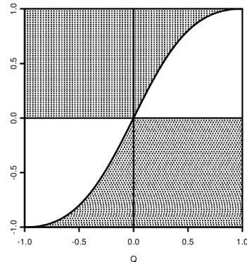
Q r1 2 -1.0 -0.5 0.0 0.5 1.0 -1 .0 -0 .5 0. 0 0. 5 1. 0
Figure 1. The Regions of Enhancement-Synergism.
of rY 2to rY 1:
Q = rY 2=rY 1: (5)
Since the designation of X1and X2is arbitrary, as long as only
one of rY 1 and rY 2 is zero, Q can be set as zero. The case
that both rY 1and rY 2 are zero will be excluded because R2is
obviously zero from (2).
Equation (5) enables us to rewrite (4) in terms of Q and r12,
and one gets r12 > g(Q) for r12 > 0 and r12 < g(Q) for
r12< 0, where g(Q) = 2Q=(1 + Q2). Equivalently, Q < q0or
Q > 1=q0for r12> 0, and Q < 1=q0or Q > q0for r12< 0,
where q0 = (1
p
1 r122 )=r12. Note that g(Q) = g(1=Q),
for Q 6= 0. Therefore, the relation between r12and Q can be
represented by the relation between r12and Q for jQj µ 1.
Fig-ure 1 presents the occurrence of (4) for combinations of r12and
Q for jQj µ 1. Those four shaded areas stand for the occurrence regions of enhancement-synergism.We believe Figure 1 is more effective for communicating the results than Figure 2 of Currie and Korabinski (1984) where the occurrence of enhancement-synergism was presented with multiple conditional plots (com-binations of rY 2and r12for selected values of rY 1).
2.2 What is the Magnitude of Enhancement-Synergism?
Instead of measuring the magnitude of enhancement-synergism with the direct difference of R2and r2
Y 1+ rY 22 , for
the purpose of simpli¢cation, we suggest using the relative co-ef¢cient of determination, denoted by H,
H = R2=(r2Y 1+ rY 22 ); (6)
which is the ratio of R2to r2 Y 1+ r
2
Y 2. A useful expression for
H is H = 1 + Q 2 2r 12Q (1 r2 12)(1 + Q2) (7)
as a function of Q and r12. A close examinationof (7) shows that
H attains its maximum 1=(1 jr12j) and minimum 1=(1+jr12j)
for Q = sign(r12) and sign(r12), respectively. The function
sign(x) returns respective value of 1, 0, or 1 if x > 0, x = 0, or x < 0. Besides, H(Q) = H(1=Q) for Q 6= 0. As in the previous discussion of g(Q), the relation between H and Q can be represented by the relation between H and Q for jQj µ 1. To visualize these facts, we plot H against Q for jQj µ 1 in Figure 2 for three different values r12 = :1, :5, and :9. (The plots for
negative values of r12are mirror images of those for positive
values.) We believe Figure 2 provides a clearer presentation of the relative magnitude and range of the enhancement-synergism condition than the plots in Freund (1988) and Figure 1 of Currie and Korabinski (1984).
2.3 How Often Does the Enhancement-Synergism Condition Occur and What is the Expected Magnitude of Enhancement-Synergism?
Because we know the enhancement-synergism condition ex-ists, it is of interest to know how often it occurs and what is the expected magnitude in terms of relative coef¢cient of termination; that is, what are P (H > 1) and E[H]? To de-termine these two quantities, we start with the derivation of the pdf of Q. Assume the true coef¢cient parameters of 1
and 2 in (1) are 1¤ and ¤2, respectively. It can be shown
from the standard assumptions that Q = Z2=Z1, where Zj =
SY j=(¼ Sj) ¹ N (· j; 1); SY j =Pni= 1(Yi Y )(Xji Xj); Sj
is the square root of S2 j =
Pn
i= 1(Xji Xj)2, j = 1 and 2,
· 1 = (¤1S1+ 2¤ S2r12)=¼ and · 2 = (2¤ S2+ 1¤ S1r12)=¼ .
Note that corr(Z1; Z2) = r12. Hence the distribution of Q is
exactly the same as the distribution of the ratio of two correlated normal random variables with mean (· 1; · 2), variance (1, 1) and
correlation r12. This is a special case of the ratio of two
corre-lated normal random variables discussed by Fieller (1932) and Hinkley (1969). Its explicit pdf and cdf were given by Hinkley (1969, eq. (1)–(3)). It appears, however, that there is no ana-lytic form for P (H > 1) = 1 P (q0 < Z2=Z1 < 1=q0) for
Q H -1.0 -0.5 0.0 0.5 1.0 0 1 2 3 4 5 6 7 8 9 10 11 r12 = 0.9 r12 = 0.5 r12 = 0.1
Figure 2. The Relation Between H and Q.
122 General
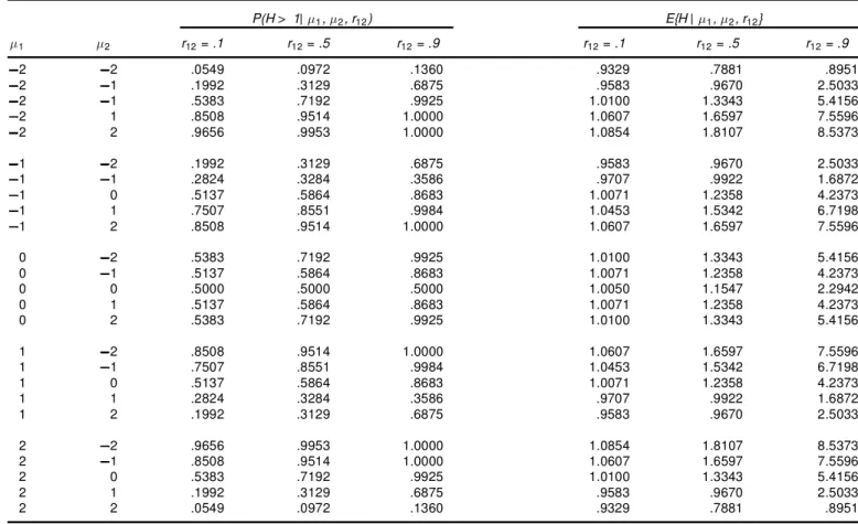
Table 1. The Occurrence Probability of Enhancement-Synergismand the Expected Relative Coefcient of Determination P(H > 1| · 1, · 2, r12) E{H| · 1, · 2, r12} · 1 · 2 r12= .1 r12= .5 r12= .9 r12= .1 r12= .5 r12= .9 2 2 .0549 .0972 .1360 .9329 .7881 .8951 2 1 .1992 .3129 .6875 .9583 .9670 2.5033 2 1 .5383 .7192 .9925 1.0100 1.3343 5.4156 2 1 .8508 .9514 1.0000 1.0607 1.6597 7.5596 2 2 .9656 .9953 1.0000 1.0854 1.8107 8.5373 1 2 .1992 .3129 .6875 .9583 .9670 2.5033 1 1 .2824 .3284 .3586 .9707 .9922 1.6872 1 0 .5137 .5864 .8683 1.0071 1.2358 4.2373 1 1 .7507 .8551 .9984 1.0453 1.5342 6.7198 1 2 .8508 .9514 1.0000 1.0607 1.6597 7.5596 0 2 .5383 .7192 .9925 1.0100 1.3343 5.4156 0 1 .5137 .5864 .8683 1.0071 1.2358 4.2373 0 0 .5000 .5000 .5000 1.0050 1.1547 2.2942 0 1 .5137 .5864 .8683 1.0071 1.2358 4.2373 0 2 .5383 .7192 .9925 1.0100 1.3343 5.4156 1 2 .8508 .9514 1.0000 1.0607 1.6597 7.5596 1 1 .7507 .8551 .9984 1.0453 1.5342 6.7198 1 0 .5137 .5864 .8683 1.0071 1.2358 4.2373 1 1 .2824 .3284 .3586 .9707 .9922 1.6872 1 2 .1992 .3129 .6875 .9583 .9670 2.5033 2 2 .9656 .9953 1.0000 1.0854 1.8107 8.5373 2 1 .8508 .9514 1.0000 1.0607 1.6597 7.5596 2 0 .5383 .7192 .9925 1.0100 1.3343 5.4156 2 1 .1992 .3129 .6875 .9583 .9670 2.5033 2 2 .0549 .0972 .1360 .9329 .7881 .8951 r12> 0, or 1 ¡ P (1=q0< Z2=Z1< q0) for r12< 0, except in
the following special case. Assume ¤
1 = 2¤ = 0, or equivalently · 1= · 2 = 0. In this
case, Q can be viewed as the ratio of two correlated standard normal variables and has a Cauchy distribution with location parameter ³ = r12and scale parameter ¶ = (1 ¡ r122 )1=2; see
Johnson, Kotz, and Balakrishnan (1994, eq. 16.1). Since its cdf is of the form FQ(q) = :5 + ¸ ¡ 1tan¡ 1f(q ¡ ³ )=¶ g, one has
P (H > 1) = 1 ¡ jFQ(q0) ¡ FQ(1=q0)j
= 1 ¡ jtan¡ 1(¡ q
0) ¡ tan¡ 1(1=q0)j=¸ = :5:
The last equality follows from the fact that ¡ q0× 1=q0= ¡ 1.
Therefore it is equallylikely to have or not to have enhancement-synergism in a two-variable regression with explanatory vari-ables that are absolutely irrelevant for describing the response variable. More importantly, this is true for all r126= 0. This
out-come may be easy to guess; however, it is not as trivial as one may think.
The actual occurrence probability of enhancement-synergism under various values of (· 1; · 2) are calculated through
numer-ical integration and are listed in Table 1 for r12= :1, :5, and :9.
In general, P (H > 1j· 1; · 2; r12) = P (H > 1j¡ · 1; ¡ · 2; r12)
and P (H > 1j· 1; ¡ · 2; r12) = P (H > 1j ¡ · 1; · 2; r12) due to
symmetry. It is also true that P (H > 1j· 1; · 2; r12) = P (H >
1j· 1; ¡ · 2; ¡ r12).
Based on the pdf of Q and (7), we can evaluate the expected relative coef cient of determination E[H] for any r12 6= 0.
Again it does not appear to have a simple analytic form and numerical integration is necessary to carry out the expectation.
Table 1 also presents the expected magnitude of enhancement-synergism in terms of H for r12 = :1; :5, and :9. In
partic-ular, when (· 1; · 2) = (0; 0), the values are 1.0050, 1.1547,
and 2.2942 for r12= :1; :5; and :9, respectively. This indicates
that the relative coef cient of determination is greater than one in “average” for all r12 6= 0 when (· 1; · 2) = (0; 0). So far
we are unable to prove that E[Hj· 1 = 0; · 2 = 0; r12] > 1
for all r12 6= 0. Moreover, Table 1 shows that the
differ-ences of E[H] among different values of (· 1; · 2) are more
dra-matic as jr12jgets larger. Overall E[Hj· 1; · 2; r12] = E[Hj ¡
· 1; ¡ · 2; r12]; E[Hj· 1; ¡ · 2; r12] = E[Hj ¡ · 1; · 2; r12] and
E[Hj· 1; · 2; r12] = E[Hj· 1; ¡ · 2; ¡ r12].
3. CONCLUSION
We provide a simpli ed and systematic view of the coun-terintuitive inequality or the enhancement-synergism condition that the coef cient of determination can exceed the sum of two squared simple correlation coef cients. The major differ-ence between our approach and others is that the relative sim-ple correlation Q and the relative coef cient of determina-tion H are the primary tools for analyzing such phenomenon rather than the original measures and their difference. The fol-lowing four major questions are studied: (1) When does the enhancement-synergism condition occur? (2) What is the mag-nitude of enhancement-synergism? (3) How often does the enhancement-synergism condition occur? (4) What is the ex-pected magnitude of enhancement-synergism? Both theoretical arguments and graphical presentations are given. Numerical ex-amples are provided to illustrate the levels of the
synergism and its dependence on the other measures. In addi-tion to the surprising enhancement-synergism condiaddi-tion itself, we point out two interesting features when the explanatory ables are absolutely irrelevant for describing the response vari-able. It is shown that even the two true coef¢cient parameters are indeed zero (¤
1 = 2¤ = 0) the occurrence probability of
the enhancement-synergismcondition is .5 for all r126= 0.
Fur-thermore, under the same assumption, it is shown numerically that the expected relative coef¢cient of determination appears to be greater than 1 for all r126= 0 and is increasing with jr12j.
[Received October 1999. Revised April 2000.]
REFERENCES
Bertrand, P. V., and Holder, R. L. (1988), “A Quirk in Multiple Regression: The Whole Regression can be Greater Than the Sum of its Parts,” The Statistician,
37, 371–374.
Cuadras, C. M. (1993), “Interpreting an Inequality in Multiple Regression,” The
American Statistician, 47, 256–258.
Currie, I., and Korabinski, A. (1984), “Some Comments on Bivariate Regres-sion,” The Statistician, 33, 283–293.
Fieller, E. C. (1932), “The Distribution of the Index in a Normal Bivariate Pop-ulation,” Biometrika, 24, 428–440.
Freund, R. J. (1988), “When is R2 > r2
y1+ r2y2 (Revisited),” The American
Statistician, 42, 89–90.
Hamilton, D. (1987), “Sometimes R2> r2
y x1+ r2y2, Correlated Variables are
not Always Redundant,” The American Statistician, 41, 129–132. (1988), “Sometimes R2 > r2
y x1+ ry x2 2, Correlated Variables are not
Always Redundant” (Reply), The American Statistician, 42, 90–91. Hinkley, D. V. (1969), “On the Ratio of Two Correlated Normal Random
Vari-ables,” Biometrika, 56, 635–639.
Johnson,N. L., Kotz, S., and Balakrishnan, N. (1994),Distributions in Statistics:
Continuous Univariate Distributions I, New York: Wiley. Johnston, J. (1991), Econometric Methods, New York: McGraw-Hill. Mitra, S. (1988), “The Relationship Between the Multiple and the Zero-Order
Correlation Coef¢cients,” The American Statistician, 42, 89.
124 General