財務比率與總體經濟因素對財務危機預警之影響

國

立

交

通

大

學

管理學院碩士在職專班財務金融組

碩

士

論

文

財務比率與總體經濟因素對財務危機預警之影響

The Impact of Financial Ratios and Macro-variables

on

Financial Distress Determination

研 究 生：劉榮宗

指導教授：李正福 教授

財務比率與總體經濟因素對財務危機預警之影響

The Impact of Financial Ratios and Macro-variables

on

Financial Distress Determination

研 究 生：劉榮宗 Student：Rong-Chung Liu

指導教授：李正福 博士 Advisor：Dr. Cheng-Few Lee

國 立 交 通 大 學

管理學院碩士在職專班財務金融組

碩 士 論 文

A Thesis

Submitted to Department of College of Management National Chiao Tung University

in partial Fulfillment of the Requirements for the Degree of

Master in

Finance

September 2010

Hsinchu, Taiwan, Republic of China

i

財 務 比 率 與 總 體 經 濟 因 素 對 財 務 危 機 預 警 之 影 響

學生：劉榮宗

指導教授

：

李正福 博士

國立交通大學管理學院碩士在職專班財務金融組

摘

要

本論文之主要目的在研究財務比率與總體經濟因素對財務危機預警之影響。根據公 司的財務比率資料以及總體經濟相關指標，以Logit模型來研究公司的財務狀況和預測未 來的破產機率。本文用1992到2007年的歷史資料來估計建立模型參數，並將建立之預測 模型，針對2008-2009年期間樣本公司分析違約機率來驗證所建立財務預測模型之準確 性。本論文採用加入與未加入總體經濟因素的兩種模型，來判斷經濟指標對財務危機預 警模型之影響，實證結果顯示出總體經濟因素對於預測模型的重要性。此研究指出對於 破產預測、投資組合管理和公司的內部與外在表現分析的應用可能性，並可提供給投資 者做參考避免重大損失發生。 關鍵詞：財務危機預警模型；Logit；總體經濟因素

ii

The Impact of Financial Ratios and Macro-variables

on

Financial Distress Determination

Student：Rong-Chung Liu

Advisor

：

Dr. Cheng-Few Lee

Graduate Institute of Finance

College of Management

National Chiao Tung University

ABSTRACT

The purpose of this paper is to investigate the impact of financial ratios and macroeconomic variables on financial distress. According to the information with respect to the financial ratios and macroeconomic related indicators, Logit model can research on the firms’ financial situation and predict the bankruptcy probability in the future. The parameters are estimated by the historical data from 1992 to 2007, and then the model can be constructed and verified by the evaluation the default probability of the firms during 2008-2009 and the detection whether firms fail or not. This paper adopts two models with and without macroeconomical factors to detect the influence of macroeconomic indicators on financial distress prediction model. The empirical results show the importance of macroeconomic factors within the failure prediction model. This study indicates the potential important application on the failure prediction, management portfolio and the internal and external performance analysis of the companies. Moreover, this paper provides the suggestion to investors and avoids the enormous loss occurring.

iii

Table of Contents

Chinese Abstract ………

i

English Abstract ……… ii

Table of Contents ………

iii

List of Tables ………

iv

List of Figures

………

v

I. Introduction………

1

II. Literature

Review………

3

III. Methodology………

7

3.1 Logit

Model………

7

3.2 Cut-off

Point………

19

IV. Experiment………

11

4.1

Definition of Financial Distress………

11

4.2 Sample

Data………

11

4.3 Factors

Choosing………

12

4.3.1 Financial

Ratios………

12

4.3.2 Macroeconomic

Factors………

15

V. Empirical

Results………

17

5.1 Without

Macroeconomic

Factors………

17

5.2

With Macroeconomic Factors.………

21

5.3 Prediction

Sample

Performance

24

VI. Conclusion………

29

Appendix A

………

31

Appendix B

………

33

iv

List of Tables

Table 3.1 The Quality of the KS Value………...10

Table 4.1 Number of Sample Companies………12

Table 4.2 The Summary of Chosen Financial Ratios………..14

Table 4.3 Descriptive Statistics of Financial Ratios………14

Table 4.4 The Summary of Chosen Macroeconomic Factors……….15

Table 4.5 Correlation Coefficient of Macroeconomic Factors………15

Table 4.6 Descriptive Statistics of Macroeconomic Factors………...16

Table 5.1 Coefficient Estimate of Model 1……….18

Table 5.2 The Process of Finding Maximum KS Value……….19

Table 5.3 Model 1 Performance of Estimation Sample ……….20

Table 5.4 Coefficient Estimate of Model 2……….22

Table 5.5 The Process of Finding Maximum KS Value……….23

Table 5.6 Model 2 Performance of Estimation Sample………..24

Table 5.7 Model 1 Performance of Prediction Sample………...25

v

List of Figures

Figure 5.1 KS Value in Model 1……….20

Figure 5.2 KS Value in Model 2……….24

Figure 5.3 Probability of Model 1 (Failed) ………27

Figure 5.4 Probability of Model 1 (Non-failed) ……….27

Figure 5.5 Probability of Model 2 (Failed) ……...……….28

1   

I. Introduction

The world was stunned when East Asia, the highest growth region during 1990s, was broken by a banking crisis in 1997 and the burst of Internet bubbles followed in 2000. Recently, since subprime mortgage crises broke out in August, 2007, economical recession occurs again and enormous companies encounter financial difficulties and defaults. The investors are afraid of vast loss due to liquidity and bankruptcy risk of financial institutions and firms. The research related to credit risk and financial distress prediction model hence isof vigorousness development to protect investors from enormous loss.

The default of a firm can be detected according to information, for example, financial statement, firm’s announcement, financial market or economic index. According to that significant information, the investors can avoid the loss of false portfolio through the investment of healthy firms. The purpose of this paper is to provide a convictive model with financial information and economic indexes, evaluate the default probability of companies, and enhance the accuracy of failure prediction for investors. Then the investors can refer to result of this model for the choice of portfolio.

Prior literatures provide several methods to calculate the default probability and to forecast the firm’s situation in the future. The prediction models can be categorized into univariate discriminant analysis (Beaver, 1966), multivariate discriminant analysis (Altman, 1968), Logit model (Ohlson, 1980), Probit model (Zmijewski, 1984). This paper based on Logit model and a proper cut-off point, could predict the default possibility for investors as the suggestion of investment. Although previous paper effectively incorporated historical financial data into model and presented significant practical results, the various financial ratios changing over time are neglected. The macroeconomic factors would influence microeconomic variables seriously, and then the accuracy of models would be unstable and unconvinced. In hence, this paper engages in the combination of macroeconomic variables and financial ratios to analysis whether firm would fail or not. 

2

This paper is organized as follows. Starting from introduction of purpose and motivation about prediction of failure firms, next section expresses the previous literatures related to our methodology and provides prior studies which deal with economical factors. Section 3 proposes our model and section 4 states the data and the explanatory variables. Section 5 shows the empirical results and analysis accuracy of prediction with and without macroeconomic factors. Finally, section 6 would make a conclusion and discuss the imperfections of this thesis and the recommendation for the future research.

  3   

II. Literature Review

Financial distress prediction models can be approximately classified into many categories. The investigation of corporate failure prediction models begins from univariate analysis (Beaver, 1966) and multivariate discriminant analysis (Altman, 1968). One of the classic works in the field of bankruptcy classification was provided by Beaver (1966). Beaver firstly employed dichotomous classification test to build financial distress prediction model. This univariate analysis including bankruptcy indicators set the stage for the multivariate attempts, which replace several variables by one factor to detect failed firms.

The pioneering work in the area of bankruptcy prediction using multivariate techniques is generally contributed to Altman (1968). The multivariate discriminant analysis (hereafter called MDA) improves the drawback of univariate analysis which only uses one financial ratio as the variable in the model. The discriminant model included five explanatory variables that affect firm’s liquidity, profitability, leverage, solvency and activity and capture various financial dimensions of the firm. According to these predictable factors, Altman regression model calculates the discriminant score to distinguish whether the firm defaults or not. Very briefly, the variables in the regression model (called Z-score model) are: 1. Net working capital/total assets, 2. Retained earnings/total assets, 3. Earnings before interest and taxes/total assets, 4. Market value equity/book value of total debt, and 5. Sales/total assets. In the evidence from MDA model, Altman shows the discriminant score (Z-score) 2.675 as the cut-off point which could distinguish the sound firms from the default firms. If firm’s Z-score larger (smaller) than 2.675, the firm is classified as a non-failed firm (a failed firm).

Specifically, according to the sample of 33 bankrupt and non-bankrupt firms, Altman's linear MDA model was able to classify accurately 95 percent of the original sample using financial data one reporting period prior to bankruptcy. However, the accuracy of prediction in Z-score model declines as the length of time increasing. The classification accuracy

4

declined to less than 72 percent for data two years prior to bankruptcy and to 36 percent for data dating from five years before bankruptcy. Subsequent research (Deakin, 1972; Blum 1974; Sinkey, 1975) largely focused on improvements in the selection of explanatory variables which yielded the better result in terms of prediction accuracy over the 1968 Altman model.

The previous studies mostly use the 1968 Altman model as a benchmark because of its popularity in the literature. Later, Altman, Haldeman, and Naraynana (1977) constructed a second generation model with the enhancement to the original Z-score approach. Due to economical factors vary with time, the adjusted Z-score model called ZETA model incorporated seven significant variables with respect to business failures. The seven factors are Return on assets (ROA), Stability of earnings, Debt service, Cumulative profitability, Liquidity, Capitalization, and Size. The variables are respectively measured by (1) earnings before interest and taxes/total assets, (2) the standard error of estimate around a ten-year trend in ROA, (3) earnings before interest and taxes/total interest payments, (4) retained earnings/total assets, (5) current ratio, (6) common equity/total capital, and (7) total assets. The ZETA model successfully enhanced the effectiveness in classifying bankrupt firms up to five years prior to failure on the 53 sample of manufacturers and retailers. The results show the prediction of accuracy is 96% in one year and 70% in five years prior to failure.

Generally, we use qualitative choice model when the dependent variables in the regression belong to discrete data, for example, dependent variable given 1 as failure and otherwise given 0. Ohlson (1980) firstly adopts Logit model to calculate the default probability. Logit model assumes that the probability of event happening follows Logistic distribution. The purpose of using Logit methodology is to avoid some well known problems related to MDA. The unprecedented assumption of distribution in financial distress prediction improved the drawback of MDA model which only can predict failure but cannot evaluate the default probability. The output of the application of MDA model is a score (Z-score) which is

5

indirectly related to decision policy of bankruptcy. Thus the misclassification may result from decision problem. Furthermore, there are certain statistical requirements in MDA model imposed on the distributional properties of the predictors. For instance, the variance-covariance matrices of the predictors should be the same for failed and non-failed firms groups. Also, the “matching” procedures in MDA model constrained the sample number. Thus, the use of Logit analysis essentially avoids all of the problems discusses associated with MDA. That is why Ohlson can choose sample with 105 failed firms and 2058 non-failed firm in contrast with 53 firms in each groups. In Logit model, nine variables are: 1. Log( total assets/GNP price-level index), 2. Total liabilities/total assets, 3. Working capital/total assets, 4. Current liabilities/current assets, 5. Bankruptcy dummy variable (one if total liabilities exceeds total assets, zero otherwise), 6. Net income/total assets, 7.Funds provided by operations/total liabilities, 8. Net income dummy variable (one if net income was negative for the last two years, zero otherwise), and 9. Change in net income. Under 0.5 as cut-off point, the predictions of accuracy are 96.12%, 95.55% and 92.84% related to the failure sample in period 1977, 1978, and 1977~1978 respectively.

Previous studies subsequently extend the application of Logit model to financial distress prediction. Lau (1987) classifies companies into five groups according to the soundness situation. Queen and Roll (1987) separate the eliminated firms into two groups according to the reason for emerge or default. Then analyze these firms via Logit model with five variables. Hopewood, Mckeown and Mutchler (1994) state the prediction of Logit model consistent with the accountant’s opinion. Platt and Platt (1990) consider that the financial ratios would vary unsteadily over time because of economical factors such as business cycle, inflation, and interest rate. They assert that the accuracy of prediction would increase if focusing on the firms in the same industry. Hwang, Lee and Liaw (1997) predict the bankruptcy of bank in America during the period from 1985 to 1988 via Logit model with 48 financial ratios as variables. Kane, Patricia and Richardson (1998) investigate the influence of economic

6

recession on financial distress prediction. The evidence illustrates the importance of economics recession factor and shows the significance of cash flow/ total assets and net income/total assets in Logit model. Compared to the occurrence of event following Logistic distribution in Logit model, Probit model and Probabilistic model assume the occurrence of event following Normal distribution and Cauchy distribution respectively. The unprecedented application of Probit model to financial distress prediction originated with Zmijewski (1984). However, in general, Logit model easily deals with the data, most papers usually construct financial distress prediction model based on Logit model.

The previous research on the failure of company mostly focuses on financial ratios to enhance the accuracy of financial distress prediction. However, only use firm’s internal information such as financial statement seems not enough to predict firm’s situation due to the significant effect of economical factors on these microeconomic variables (Platt and Platt, 1990; Kane, Patricia and Richardson, 1998). Suetorsak (2006) examines interactions between micro and macro variables in explaining the risk positions of East Asian banks. The analysis shows that macroeconomic policies significantly impacted the bank’s micro-economic decision. Suetorak (2006) states that macro conditions and government policies influences bank’s reactions to their microeconomic variables and the level of risk they take. Therefore, the macroeconomic factors are of importance in the investigation on the bankruptcy of firms. In this paper, financial ratios combined with macroeconomic factors engage in the analysis of the default and failure companies to increase the accuracy of prediction.

  7   

III. Methodology

In this study, we established a financial distress model by Logit Model. We tried to verify whether macroeconomic factors affect financial distress model or not. Therefore we used financial ratios as our basic factors of inputs, and compared the performance of models which without macroeconomic factors and the other with macroeconomic factors. In this section, we start with introducing the methodology used in this study.

3.1 Logit Model

The outcomes of the financial distress are between two discrete alternatives, failed or non-failed. Thus the binary choice model is an appropriate method for us to apply. The dependent variable Yk takes the value of 1 when the company suffers financial distress, and takes the value of 0 when otherwise. Logit Model assumes that the bankruptcy probability has a Logistic distribution. In a dummy regression equation of company k, suppose the continuously dependent variable * k y represent the possible situation of financial distress, and k

x ’s are its linear independent variables. The event will happen when the continuously

dependent variable crosses a value of threshold, say T. k y is the value we can observe. For

example, let T = 0 as a divide such that the firm encounters financial distress if the dependent variable value is negative and the sound firm if the dependent variable value is positive. The equation can be expressed as following:

  Assume k ε follows the logistic distribution. Then we have the conditional probability of

8 1 ( 1| ) ( m 0) k k k ik ik k i p P y x P α β x ε = = = = +

∑

+ > 1 ( _k m _{ik ik}) i P ε α β x = = > − −

∑

1 ( _k m _{ik ik}) i P ε α β x = = ≤ +

∑

1 ( ) 1 1 m ik ik i x e α β = − + = ∑ + (3-3)

Or written in the form of logit function of bankruptcy probability

1 ln 1 m k ik ik i k p x p α = β ⎛ _⎞⎟ ⎜ _{⎟ = +} ⎜ _⎟ ⎜ ⎟ ⎜ − ⎝ ⎠

∑

(3-4) In order to figure out the probability of this model, we have to estimate the parameters α

and β . In the linear regression models, the OLS (ordinary least squares) is frequently used ik

to estimate the parameters. However, we cannot use the OLS to estimate the coefficients due to bias. Thus, we use the MLE (maximum likelihood estimator) to estimate. Suppose Y1,

Y2, …, Yn are identically independent distribution of Bernoulli(pk). Then we have the probability

1

( ) yk(1 ) yk

k k k

f y = p −p − (3-5)

and the likelihood function is:

1 1 ( , | ) k(1 ) k n y y k k k L α β y p p − = =

∏

− (3-6)

By equation (3-6), we can get the log-likelihood function as:

[

]

1 1 ln ( , | ) ln k(1 ) k n y y k k k L α β y p p − = ⎡ ⎤ ⎢ ⎥ = _⎢ − _⎥ ⎣

∏

⎦

9

[

]

1 ln( ) (1 ) ln(1 ) n k k k k k y p y p = =

∑

+ − − 1 ln ln(1 ) 1 n k k k k k p y p p = ⎡ ⎛_{⎜ ⎞⎟} ⎤ ⎢ _⎟ ⎥ = _⎢ ⎜_{⎜⎜ − ⎟⎟}+ − _⎥ ⎝ ⎠ ⎢ ⎥ ⎣ ⎦

∑

1 1 1 1 ln 1 1 m ik ik i m ik ik i x n m k ik ik x k i e y x e α β α β α β = = + + = = ⎡ ⎛_{⎜ ∑ ⎞⎟}⎤ ⎢ _{⎛ ⎞ ⎜ ⎟⎥⎟} ⎢ _{⎜ ⎟} ⎜_{⎜ ⎟⎟}⎥ = _⎢⎢ _⎝⎜_⎜ + _⎠⎟⎟⎟+ ⎜_⎜⎜ − ⎟_⎟⎥_⎥ ⎟ ∑ _⎟ ⎜ ⎢ _{⎜⎝ + ⎠⎥⎟} ⎢ ⎥ ⎣ ⎦

∑

∑

1 1 1 ln 1 m ik ik i n m x k ik ik k i y x e α β α β = + = = ⎡ _{⎛ ⎞} ⎛_{⎜ ∑ ⎞⎟}⎤ ⎢ _{⎜ ⎟ ⎜ ⎟⎥⎟} ⎢ ⎥ = _{⎢ ⎝}⎜_⎜ + _⎟⎠⎟_⎟− _⎜⎜_⎜ + _⎟⎟_⎥ ⎟⎟ ⎜⎝ ⎠ ⎢ ⎥ ⎣ ⎦

∑

∑

(3-7) where yk equals to one if the firm goes bankruptcy and equals to zero otherwise.

We take differentiating with respect to α β β, , ,...,_{1 2} β for maximizing equation (3-7), and _m

set it to zero. Then, we can get the normal equations:

[

]

[

]

1 1 1 1 1 1 ln ( , | ) 0 1 ln ( , | ) 0 1,..., 1 m ik ik i m ik ik i m ik ik i m ik ik i x n k x k x n k jk x k j L y e y e L y e y x j m e α β α β α β α β α β α α β β = = = = + + = + + = ⎧ ⎡ ⎤ ⎪ _∑ ⎪ _{⎢ ⎥} ⎪∂ ⎪ ⎢ ⎥ ⎪ _{= ⎢ − ⎥=} ⎪⎪ _{∂ ⎢ ∑ ⎥} ⎪⎪ ⎢ ₊ ⎥ ⎪ _{⎣ ⎦} ⎪⎨ ⎪ ⎡ ⎤ ⎪ _{⎢ ∑ ⎥} ⎪⎪∂ _{⎢ ⎥} ⎪ _{= − = =} ⎪ ⎢ ⎥ ⎪ _{∂ ⎢ ⎥} ⎪ ∑ ⎪ _{⎢ ⎥} ⎪ + ⎪ ⎣ ⎦ ⎩

∑

∑

(3-8)

By solving this equation (3-8), we can get the parameters α β β, , ,...,_{1 2} β . _m

3.2 Cut-off point

After implementing the Logit Model, we can classify every firm as default group or non-default group by using a cut-off point. Traditionally, we use 0.5 as our cut-off point. This means that if the predicted bankruptcy probability of a company is higher than 0.5, we will classify the firm as the default group; if the predicted bankruptcy probability of a company is

10

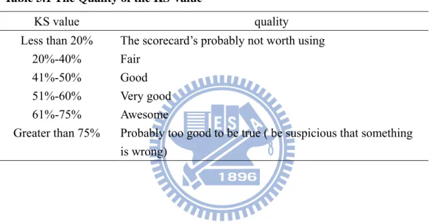
lower than 0.5, we will classify the firm as the non-default group. But whether the best value of cut-off point is 0.5 is a debatable problem. So we then employ the maximum KS value method (Mays,2001) to find the better cut-off point. KS value is the difference between cumulated percentages of default firm’s number and the non-default one. The range that max KS value falls in is the cut-off point we want. Table3.1 shows the general guide to the quality of the KS.

Table 3.1 The Quality of the KS Value

KS value quality

Less than 20% The scorecard’s probably not worth using 20%-40% Fair

41%-50% Good

51%-60% Very good

61%-75% Awesome

Greater than 75% Probably too good to be true ( be suspicious that something is wrong)

  11   

IV. Data

This section can be separated into three parts. The first part states the definition of financial distress according to TEJ database; the part about sample data expresses the period and the number of the samples; the final part is the independent factors choosing.

4.1 Definition of Financial Distress

A company encounters financial difficulties and defaults when it fails to service its debt obligation. Many researchers have studied corporate bankruptcy; different people have come up with different definitions that basically reflect their special interest in the field. In this study, we will use the definitions of financial distress and quasi financial distress in TEJ database as default event.

4.2 Sample Data

Our sample firms must be listed on Taiwan Stock Exchange Corporation (TSE) or GreTai Security Market (GTSM or OTC). Because the characteristics of banking, security and insurance industries are different from others, we exclude these industries from our sample firms. Besides, we also exclude the firms of which financial reports are incomplete.

We collect data of the sample firms from TEJ database. The study period is 1992-2009. If the firms experienced the financial distress situations mentioned in section 4.1 during this period, we classify these firms as default group. The non-default firms are firms that remain trading on TSE or GTSM during 1992-2009. The healthy or non-default firms we select are chosen on 1:1 basis. The industry and size of the healthy firm match with the default one. That is, the non-default firm’s industry and firm size is similar to the default one.

We have two kinds of data, financial ratios and macroeconomic factors. We choose financial ratios from financial year report one year before the firms suffering from financial

12

distress. We use sum of season macroeconomic factors. If financial distress breaks out in time t year, then we collect the first and second quarter of time t year, third and fourth quarter of the last year of time t year, and then sum these four quarts data together.

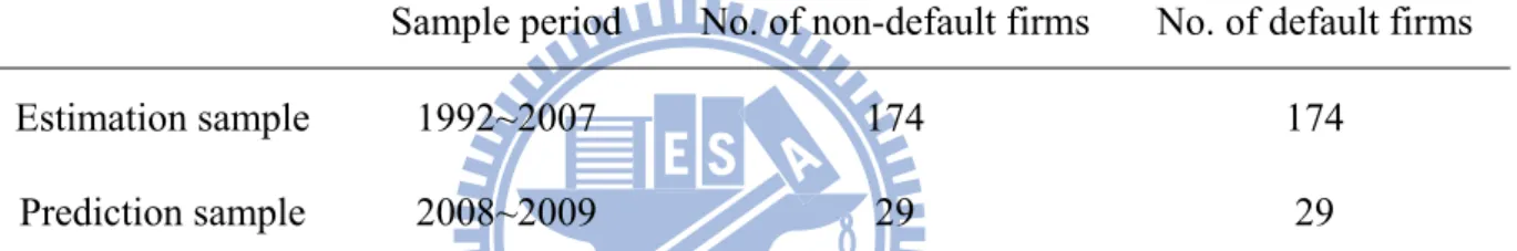
We use the observations between 1992 and 2007 as the estimation sample, and the observations from 2008 to 2009 as the prediction sample validation group to examine the model’s accuracy. Finally, there are 174 non-default firms and 174 default firms in the estimation sample, and 29 non-default firms and 29 default firms in the prediction sample. The number of estimation sample and prediction sample firms is shown in Table 4.1.

Table 4.1 Number of Sample Companies

Sample period No. of non-default firms No. of default firms

Estimation sample 1992~2007 174 174

Prediction sample 2008~2009 29 29

The data comes from TEJ database which the period is from 1992 to 2009. The sample firms are listed either on Taiwan Stock Exchange Corporation (TSE) or on GreTai Security Market (GTSM or OTC).

4.3 Factors choosing

The chosen independent variables can be classified into two kinds of variables, that is, financial ratios and macroeconomic factors respectively. The detail of these factors would be discussed subsequently.

4.3.1 Financial ratios

In this study, we collect inputs according to six category measures as follows.

1. Long-term solvency measure

Long-term solvency ratios are intended to address the firm’s long-run ability to meet its obligations, or more generally, its financial leverage. We choose “Debt Ratio” and

13

“ Equity Long-term liabilities

Fix assets +

” in this category.

2. Short-term solvency or Liquidity measure

Short-term solvency ratios as a group are intended to provide information about a firm’s liquidity. The primary concern is the firm’s ability to pay its bills over the short run without undue stress. Consequently, these ratios focus on current assets and current liability. We choose “Current Ratio” and “Quick Ratio” (Acid Test Ratio) in this category.

3. Asset management or Turnover measure

Turnover ratios are intended to describe how efficiently, or intensively, a company uses its assets to generate sales. We choose “Inventory Turnover Ratio”, “Receivables Turnover Ratio”, and “Total Asset Turnover Ratio” in this category.

4. Profitability measure

Profitability measures are intended to measure how efficiently the company uses its assets and how efficiently the company manages its operations. The focus in this group is on net income. We choose “Profit Margin” and “Return on Total Assets” in this category.

5. Cash flow measure

A firm’s cash flow measures reveal whether the firm makes money or not, and whether the money generated in this period can meet its obligations. We choose “Cash Ratio” and “Change in Cash flow” in this category.

6. Firm’s Size

The company with different size will have different ability of overcome financial distress. We use the natural log of firm’s size as an input.

Table 4.2 shows the code and calculation of the financial ratios used in this paper. Table 4.3 shows the descriptive statistics of the financial ratios.

14

Table4.2 The Summary of Chosen Financial Ratios

Category Code Variable Equation

Solvency

measure FR1 Debt Ratio

Total Liabilities Total Assets

FR2 Equity Long-term liabilities

Fix assets +

Liquidity

measure FR3 Current Ratio

Current Assets Current Liabilities

FR4 Quick Ratio Current Assets Inventory

Current Liabilities − Turnover measure FR5 Inventory Turnover Ratio

Cost of good sold Inventory FR6 Receivables Turnover

Ratio

Sales

Accounts receivable

FR7 Total Asset Turnover Ratio

Sales Total assets

Profitability

measure FR8 Profit Margin

Net income Sales

FR9 Return on Total Assets Net income

Total assets

Cash flow

FR10 Cash Ratio Cash

Current liabilities

FR11 Change in Cash flow

Size FR12 Size Ln(Size)

The total number of variables is twelve. The solvency ability is measured by debt ration and (equity + long-term liabilities) / fix assets; the liquidity ability is measured by current ratio and quick ratio; the turnover ability is measured by inventory turnover ratio, receivable turnover ratio and total asset turnover ratio; the profitability is measured by profit margin and return of total assets (ROA); the cash flow aspect is measured by cash ratio and change in cash flow; the size measure equation is the log of size value.

Table4.3 Descriptive Statistics of Financial Ratios

Variable Mean Std Maximum Minimum

FR1 53.08892 21.49304 175.25 1.82

FR2 921.7876 4430.586 75199.76 -211.05

FR3 169.0488 171.9555 1732.41 10.56

FR4 104.9144 157.3101 1730.63 1.59

15 FR6 9.051305 31.01726 587 -1.48 FR7 0.882635 0.707633 4.73 -0.03 FR8 -34.4377 241.0873 73.67 -3668 FR9 -1.27308 18.08898 66.5 -93.38 FR10 0.151685 0.602335 4.869454 -1.61291 FR11 -155772 2812215 10869450 -4.6E+07 FR12 14.93189 1.405555 19.48802 10.79561

The variable codes are explained in Table 4.2.

4.3.2 Macroeconomic factors

In this study, we choose eight macroeconomic indicators which are listed in table 4.4. The correlation of these indicators must not too large. So we check the correlations of these factors. Table 4.5 shows the coefficient correlation of them. Table 4.6 shows the descriptive statistics of macroeconomic indicators.

Table4.4 The Summary of Chosen Macroeconomic Factors

Code Variable

MF1 Real Estate Determine Score MF2 Monitoring Indictors Score MF3 Leading Index

MF4 Floor area of Building Permit - Taiwan (Epd) MF5 Saving Rate--R.O.C(YEAR)

MF6 Unemployment Rate – U.S.A.

MF7 New privately owned housing started-U.S.A. MF8 Import Goods – U.S.A.

MF1 data comes from Architecture and Building Research Institution, Ministry of the Interior; MF2 to MF5 measures are from Council for Economic Planning and Development; MF6 data is from US Department of Labor; MF7 data is from US Census Bureau; and MF8 data is from United States International Trade Commission (USITC). All factors are annual datum.

Table4.5 Correlation Coefficient of Macroeconomic Factors

MF1 MF2 MF3 MF4 MF5 MF6 MF7 MF8 MF1 1.0000 0.6458 0.1035 0.6187 0.0218 -0.0076 0.4032 -0.0111 MF2 0.6458 1.0000 0.0380 0.6134 0.1856 -0.1030 0.3590 -0.0687

16 MF3 0.1035 0.0380 1.0000 0.0451 -0.1043 -0.3651 0.3019 0.9850 MF4 0.6187 0.6134 0.0451 1.0000 0.3073 0.0924 0.2350 -0.0457 MF5 0.0218 0.1856 -0.1043 0.3073 1.0000 0.3831 -0.4929 -0.0833 MF6 -0.0076 -0.1030 -0.3651 0.0924 0.3831 1.0000 -0.6188 -0.3407 MF7 0.4032 0.3590 0.3019 0.2350 -0.4929 -0.6188 1.0000 0.1965 MF8 -0.0111 -0.0687 0.9850 -0.0457 -0.0833 -0.3407 0.1965 1.0000 The codes MF1 to MF8 can be referred to Table 4.4 which shows the detail of macroeconomic factors.

Table4.6 Descriptive Statistics of Macroeconomic Factors

Variable Mean Std Maximum Minimum

MF1 40.84211 8.98309 60 27 MF2 92.15789 21.92478 135 48 MF3 300.5842 72.86198 423.7 193.9 MF4 9049.105 2984.417 13611 4134 MF5 27.13158 1.636847 31.25 24.15 MF6 22.28947 4.401375 31.4 16.2 MF7 5908.421 1417.039 7916 2489 MF8 380578.9 165694 704411 164530 The codes MF1 to MF8 can be referred to Table 4.4 which shows the detail of macroeconomic factors.

  17   

V. Empirical Result

In this study, we compare the financial distress models with and without macroeconomic factors. We use “Model 1” represent the model without macroeconomic factors, and “Model 2” represent the model with macroeconomic factors. In section 5.1, we show the estimation result of Model 1. In section 5.2, we show the estimation result of Model 2. In section 5.3, we show the performance of prediction sample and compare the difference of the two models.

5.1 Without Macroeconomic factors

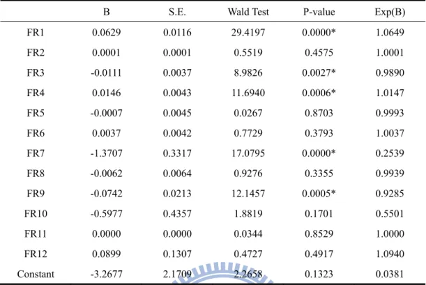
In section 3.1, we have introduced the Logit Model method. Equation (3-3) shows the probability concept of Logit Model. We use MLE to estimate the coefficients in Logit model, these coefficient estimates of model 1 is shown in Table 5.1. The regression for company k is as following

 

where FR1 is debt ratio, FR2 is equity plus long-term liabilities over fix assets, FR3 is current ratio, FR4 is quick ratio, FR5 is inventory turnover ratio, FR6 is receivables turnover ratio, FR7 is total asset turnover ratio, FR8 is profit margin, FR9 is return on total assets, FR10 is cash ratio, FR11 is change in cash flow, FR12 is ln(size).

So the probability equation of company k is

  According to the parameters estimated in Table 5.1, the regression of the equation (5-1) is as following:

18

Table5.1 Coefficient Estimate of Model 1

B S.E. Wald Test P-value Exp(B)

FR1 0.0629 0.0116 29.4197 0.0000* 1.0649 FR2 0.0001 0.0001 0.5519 0.4575 1.0001 FR3 -0.0111 0.0037 8.9826 0.0027* 0.9890 FR4 0.0146 0.0043 11.6940 0.0006* 1.0147 FR5 -0.0007 0.0045 0.0267 0.8703 0.9993 FR6 0.0037 0.0042 0.7729 0.3793 1.0037 FR7 -1.3707 0.3317 17.0795 0.0000* 0.2539 FR8 -0.0062 0.0064 0.9276 0.3355 0.9939 FR9 -0.0742 0.0213 12.1457 0.0005* 0.9285 FR10 -0.5977 0.4357 1.8819 0.1701 0.5501 FR11 0.0000 0.0000 0.0344 0.8529 1.0000 FR12 0.0899 0.1307 0.4727 0.4917 1.0940 Constant -3.2677 2.1709 2.2658 0.1323 0.0381

FR1 is debt ratio, FR2 is equity plus long-tern liabilities over fix assets, FR3 is current ratio, FR4 is quick ratio, FR5 is inventory turnover ratio, FR6 is receivables turnover ratio, FR7 is total asset turnover ratio, FR8 is profit margin, FR9 is return on total assets, FR10 is cash ratio, FR11 is change in cash flow, FR12 is ln(size). In P-value column, signal * means 1% significant. The Exp(B) is the exponential value of coefficient B for the calculation of failure probability in equation (5-1).

The estimated parameters illustrate that debt ratio, current ratio, quick ratio, total asset turnover ratio, and ROA are very significant at 1%. However, other financial ratios are of insignificance.

After estimating the coefficients, we have prediction probability of every company. The following step is to find a better cut-off point in order to sort companies into failed or non-failed catalogs. We use the Maximum KS value method to select cut-off value. Table 5.2 shows the summary of selection process. Figure 5.1 shows the figure of cumulative percentage of failed and non-failed companies. The max KS value is 66.09% and in the score range of 0.35 to 0.45. Thus we choose the upper bound 0.45 as Model 1’s cut-off point.

Table 5.3 shows the performance of estimation sample using Model 1, the correct prediction percentage of failed firms is 86.21%, the correct prediction percentage of

19

non-failed firms is 79.89%, and the correct percentage of total prediction is 83.05%. Thus the prediction ability performance of the model which uses financial ratios as its inputs is well. Note that table 5.3 also implies the type I error rate is 13.79% and type II error rate is 20.11%.

Table5.2 The Process of Finding Maximum KS Value

Score range

Number Cumulative

Number Number % Cumulative % KS value F N F N F N F N 0.00～0.05 2 38 2 38 1.15% 21.84% 1.15% 21.84% 20.69% 0.05～0.10 0 26 2 64 0.00% 14.94% 1.15% 36.78% 35.63% 0.10～0.15 2 21 4 85 1.15% 12.07% 2.30% 48.85% 46.55% 0.15～0.20 4 10 8 95 2.30% 5.75% 4.60% 54.60% 50.00% 0.20～0.25 0 12 8 107 0.00% 6.90% 4.60% 61.49% 56.90% 0.25～0.30 6 10 14 117 3.45% 5.75% 8.05% 67.24% 59.20% 0.30～0.35 2 11 16 128 1.15% 6.32% 9.20% 73.56% 64.37% 0.35～0.40 3 6 19 134 1.72% 3.45% 10.92% 77.01% 66.09% 0.40～0.45 5 5 24 139 2.87% 2.87% 13.79% 79.89% 66.09% 0.45～0.50 5 4 29 143 2.87% 2.30% 16.67% 82.18% 65.52% 0.50～0.55 5 4 34 147 2.87% 2.30% 19.54% 84.48% 64.94% 0.55～0.60 12 4 46 151 6.90% 2.30% 26.44% 86.78% 60.34% 0.60～0.65 10 4 56 155 5.75% 2.30% 32.18% 89.08% 56.90% 0.65～0.70 8 4 64 159 4.60% 2.30% 36.78% 91.38% 54.60% 0.70～0.75 7 3 71 162 4.02% 1.72% 40.80% 93.10% 52.30% 0.75～0.80 10 4 81 166 5.75% 2.30% 46.55% 95.40% 48.85% 0.80～0.85 12 3 93 169 6.90% 1.72% 53.45% 97.13% 43.68% 0.85～0.90 22 2 115 171 12.64% 1.15% 66.09% 98.28% 32.18% 0.90～0.95 16 0 131 171 9.20% 0.00% 75.29% 98.28% 22.99% 0.95～1.00 43 3 174 174 24.71% 1.72% 100.00% 100.00% 0.00% total 174 174 100.00% 100.00%

The max KS value is 66.09% noted by bold number in the table and we choose the upper bound 0.45 as the cut-off point of Model 1.

20

Figure5.1 KS Value in Model 1

KS 0.00% 20.00% 40.00% 60.00% 80.00% 100.00% 120.00% 0.00～ 0.05 0.10 ～0.1 5 0.20 ～0.2 5 0.30 ～0.3 5 0.40 ～0.4 5 0.50 ～0.5 5 0.60 ～0.6 5 0.70 ～0.7 5 0.80 ～0.8 5 0.90 ～0.9 5 interval %c um ul at e failed non-failed KS value

This picture is to find the maximum KS value which is denoted by the line with triangle spots. The line with diamond spot is the cumulative percentage of failed companies and the line with square spot is the cumulative percentage of non-failed companies. The KS value is calculated by the cumulative percentage of non-failed companies minus the cumulative percentage of failed companies.

Table5.3 Model 1 Performance of Estimation Sample

Sample Number Correct Prediction Incorrect Prediction Percentage Correct Overall Correct Percentage Observed Failed 174 150 24 86.21% 83.05% Observed Non-Failed 174 139 35 79.89% Total 348 289 59

The estimation sample is to evaluate the coefficients of parameters in model 1. Based on the coefficients calculated via MLE method, the correct percentage of observed failed firms is 86.21% and the correct percentage of observed non-failed firms is 79.89%. The overall correct percentage is 83.05% where the cut-off point is 0.45.

21

5.2 With Macroeconomic factors

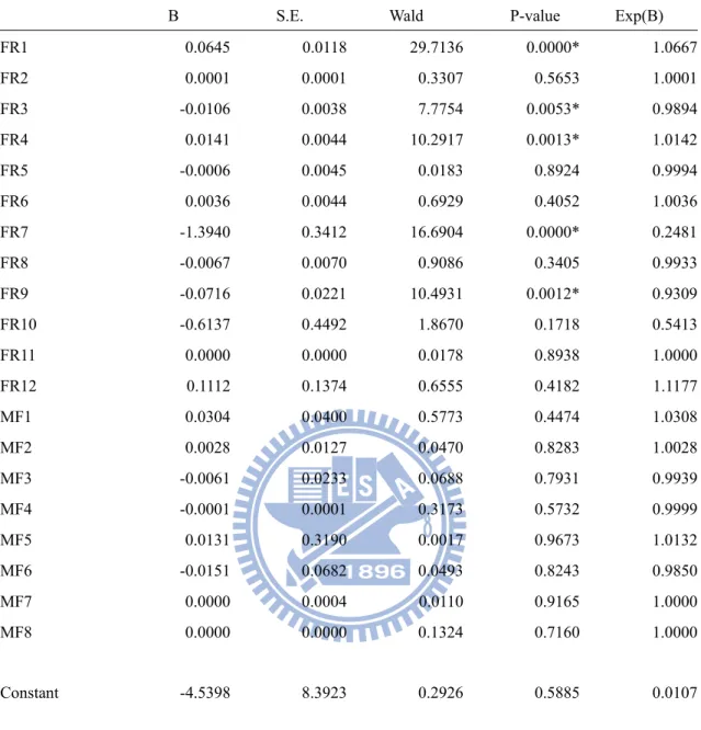
Similarly, the coefficient estimate of model 2 is shown in Table 5.4. The regression for company k is as following:

* 1 2 3 4 5 6 7 8 9 10 11 12 1 2 3 4 5 6 7 8 ˆ FR1 FR2 FR3 FR4 FR5 FR6+ FR7 FR8 FR9 FR10 FR11 FR12 MF1 MF2 MF3 MF4 MF5 MF6+ MF7 MF8 k k k k k k k k k k k k k k k k k k k k k y c β β β β β β β β β β β β λ λ λ λ λ λ λ λ = + + + + + + + + + + + + + + + + + +

where FR1 is debt ratio, FR2 is equity plus long-tern liabilities over fix assets, FR3 is current ratio, FR4 is quick ratio, FR5 is inventory turnover ratio, FR6 is receivables turnover ratio, FR7 is total asset turnover ratio, FR8 is profit margin, FR9 is return on total assets, FR10 is cash ratio, FR11 is change in cash flow, FR12 is ln(size). MF1 is real estate determine score, MF2 is monitoring indictors score, MF3 is leading index, MF4 is floor area of building permit –Taiwan (Epd), MF5 is saving rate-R.O.C(year), MF6 is unemployment rate-U.S.A., MF7 is new privately owned housing started (SA), MF8 is import goods-U.S.A.

And the probability equation of company k is

12 8 1 1 ( ) 1 1 i ik ik j jk jk k c FR MF p e β λ = = − + + = ∑ ∑ + (5-2)

where βik and λjk are the coefficients of financial ratios parameters and macroeconomic factors,

and c is the constant term.

According to the coefficients of parameters estimated in Table 5.4, the regression in equation (5-2) is as following: * ˆ 4.5398 0.0645FR1 0.0001FR2-0.0106FR3 0.0141FR4-0.0006FR5 0.0036FR6 -1.3940FR7-0.0067FR8-0.0716FR9 0.6137FR10 0.0000FR11 0.1112FR12 0.0304MF1 0.0028MF2-0.0061MF3-0.0001MF4 0.0131MF5-0.0151MF6+0.00 k y = − + + + + − + + + + + 00MF7 0.0000MF8+

22

Table5.4 Coefficient Estimate of Model 2

B S.E. Wald P-value Exp(B)

FR1 0.0645 0.0118 29.7136 0.0000* 1.0667 FR2 0.0001 0.0001 0.3307 0.5653 1.0001 FR3 -0.0106 0.0038 7.7754 0.0053* 0.9894 FR4 0.0141 0.0044 10.2917 0.0013* 1.0142 FR5 -0.0006 0.0045 0.0183 0.8924 0.9994 FR6 0.0036 0.0044 0.6929 0.4052 1.0036 FR7 -1.3940 0.3412 16.6904 0.0000* 0.2481 FR8 -0.0067 0.0070 0.9086 0.3405 0.9933 FR9 -0.0716 0.0221 10.4931 0.0012* 0.9309 FR10 -0.6137 0.4492 1.8670 0.1718 0.5413 FR11 0.0000 0.0000 0.0178 0.8938 1.0000 FR12 0.1112 0.1374 0.6555 0.4182 1.1177 MF1 0.0304 0.0400 0.5773 0.4474 1.0308 MF2 0.0028 0.0127 0.0470 0.8283 1.0028 MF3 -0.0061 0.0233 0.0688 0.7931 0.9939 MF4 -0.0001 0.0001 0.3173 0.5732 0.9999 MF5 0.0131 0.3190 0.0017 0.9673 1.0132 MF6 -0.0151 0.0682 0.0493 0.8243 0.9850 MF7 0.0000 0.0004 0.0110 0.9165 1.0000 MF8 0.0000 0.0000 0.1324 0.7160 1.0000 Constant -4.5398 8.3923 0.2926 0.5885 0.0107

FR1 is debt ratio, FR2 is equity plus long-tern liabilities over fix assets, FR3 is current ratio, FR4 is quick ratio, FR5 is inventory turnover ratio, FR6 is receivables turnover ratio, FR7 is total asset turnover ratio, FR8 is profit margin, FR9 is return on total assets, FR10 is cash ratio, FR11 is change in cash flow, FR12 is ln(size). MF1 is real estate determine score, MF2 is monitoring indictors score, MF3 is leading index, MF4 is floor area of building permit –Taiwan (Epd), MF5 is saving rate-R.O.C(year), MF6 is unemployment rate-U.S.A., MF7 is new privately owned housing started (SA), MF8 is import goods-U.S.A. In P-value column, signal * means 1% significant. The Exp(B) is the exponential value of coefficient B for the calculation of failure probability in equation (5-2).

The estimated parameters of model 2 illustrate the same results as model 1 which debt ratio, current ratio, quick ratio, total asset turnover ratio, and ROA are very significant at 1%. However, all macroeconomic factorsare not significant.

23

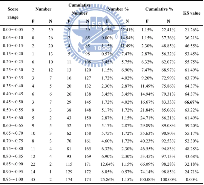
cumulative percentage of failed and non-failed companies. The max KS value is 66.67% and in the score range of 0.45 to 0.50. Thus we choose the upper bound 0.5 as Model 2’s cut-off point.

Table 5.6 shows the performance of estimation sample using Model 2, the correct prediction percentage of failed firms is 83.33%, the correct prediction percentage of non-failed firms is 83.33%, and the correct percentage of total prediction is 83.33%. Thus the prediction ability performance of the model which adds macroeconomic factors as its inputs is better than the model only use financial ratios as its inputs. From table 5.6, we know the type I error rate is 16.67% and type II error rate is 16.67%.

Table5.5 The Process of Finding Maximum KS Value

Score range

Number Cumulative

Number Number % Cumulative % KS value F N F N F N F N 0.00～0.05 2 39 2 39 1.15% 22.41% 1.15% 22.41% 21.26% 0.05～0.10 0 26 2 65 0.00% 14.94% 1.15% 37.36% 36.21% 0.10～0.15 2 20 4 85 1.15% 11.49% 2.30% 48.85% 46.55% 0.15～0.20 1 13 5 98 0.57% 7.47% 2.87% 56.32% 53.45% 0.20～0.25 6 10 11 108 3.45% 5.75% 6.32% 62.07% 55.75% 0.25～0.30 2 12 13 120 1.15% 6.90% 7.47% 68.97% 61.49% 0.30～0.35 3 7 16 127 1.72% 4.02% 9.20% 72.99% 63.79% 0.35～0.40 4 5 20 132 2.30% 2.87% 11.49% 75.86% 64.37% 0.40～0.45 6 6 26 138 3.45% 3.45% 14.94% 79.31% 64.37% 0.45～0.50 3 7 29 145 1.72% 4.02% 16.67% 83.33% 66.67% 0.50～0.55 9 3 38 148 5.17% 1.72% 21.84% 85.06% 63.22% 0.55～0.60 5 2 43 150 2.87% 1.15% 24.71% 86.21% 61.49% 0.60～0.65 9 5 52 155 5.17% 2.87% 29.89% 89.08% 59.20% 0.65～0.70 10 3 62 158 5.75% 1.72% 35.63% 90.80% 55.17% 0.70～0.75 8 3 70 161 4.60% 1.72% 40.23% 92.53% 52.30% 0.75～0.80 11 4 81 165 6.32% 2.30% 46.55% 94.83% 48.28% 0.80～0.85 12 4 93 169 6.90% 2.30% 53.45% 97.13% 43.68% 0.85～0.90 22 2 115 171 12.64% 1.15% 66.09% 98.28% 32.18% 0.90～0.95 14 1 129 172 8.05% 0.57% 74.14% 98.85% 24.71% 0.95～1.00 45 2 174 174 25.86% 1.15% 100.00% 100.00% 0.00%

24

total 174 174 100.00% 100.00%

The max KS value is 66.67% noted by bold number in the table and the score range is 0.45 to 0.5. Here we choose the upper bound 0.5 as the cut-off point of Model 2.

Figure5.2 KS Value in Model 2

KS 0.00% 20.00% 40.00% 60.00% 80.00% 100.00% 120.00% 0.00～ 0.05 0.10 ～0.1 5 0.20 ～0.2 5 0.30 ～0.3 5 0.40 ～0.4 5 0.50 ～0.5 5 0.60 ～0.6 5 0.70 ～0.7 5 0.80 ～0.8 5 0.90 ～0.9 5 interval %c um ul at e _failed non-failed KS值

This picture is to find the maximum KS value which is denoted by the line with triangle spots. The line with diamond spot is the cumulative percentage of failed companies and the line with square spot is the cumulative percentage of non-failed companies. The KS value is calculated by the cumulative percentage of non-failed companies minus the cumulative percentage of failed companies.

Table5.6 Model 2 Performance of Estimation Sample

Sample Number Correct Prediction Incorrect Prediction Percentage Correct Overall Correct Percentage Observed Failed 174 145 29 83.33% 83.33% Observed Non-Failed 174 145 29 83.33% Total 348 290 58

The estimation sample is to evaluate the coefficients of parameters in model 2. Based on the coefficients calculated via MLE method, the correct percentage of observed failed firms is 83.33% and the correct percentage of observednon-failed firms is 83.33%. The overall correct percentage is 83.33% based on the cut-off point 0.5.

25

In previous sections, we have figure out the coefficients and cut-off point. The coefficients of Model 1 are shown in Table 5.1; the coefficients of Model 2 are shown in Table 5.4; the cut-off point of Model 1 is 0.45; the cut-off point of Model 2 is 0.50. So we use these information to see how the prediction performance of the two models.

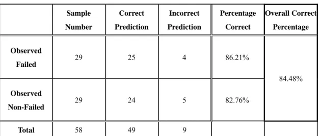
Table 5.7 shows the prediction performance of Model 1. The correct prediction percentage of failed firms is 86.21%, the correct prediction percentage of non-failed firms is 82.76%, and the correct percentage of total prediction is 84.48%. The type I error rate is 13.79% and type II error rate is 17.24%.

Table 5.8 shows the prediction performance of Model 2. The correct prediction percentage of failed firms is 86.21%, the correct prediction percentage of non-failed firms is 86.21%, so the correct percentage of total prediction is also 86.21%. The type I error rate is 13.79% and type II error rate is 13.79%, too.

Therefore, the model with macroeconomic factors is better than the model without ones. This result proves that the factor of macroeconomic affects firms’ financial situation in Logit default model.

Table5.7 Model 1 Performance of Prediction Sample

Sample Number Correct Prediction Incorrect Prediction Percentage Correct Overall Correct Percentage Observed Failed 29 25 4 86.21% 84.48% Observed Non-Failed 29 24 5 82.76% Total 58 49 9

The prediction sample is to verify the currency of model 1. The correct percentage of observed failed firms is 86.21% and the correct percentage of observed non-failed firms is 82.76%. The overall correct percentage is 84.48% based on the cut-off point 0.45.

26

Table5.8 Model 2 Performance of Prediction Sample

Sample Number Correct Prediction Incorrect Prediction Percentage Correct Overall Correct Percentage Observed Failed 29 25 4 86.21% 86.21% Observed Non-Failed 29 25 4 86.21% Total 58 50 8

The prediction sample is to verify the currency of model 2. The correct percentage of observed failed firms is 86.21% and the correct percentage of observed non-failed firms is 86.21%. The overall correct percentage is 86.21% based on the cut-off point 0.5.

We also compare the probabilities of the 29 prediction sample in 3-year before financial distress occur. Let year t be the time of financial distress occurs. Figure5.3 to figure5.6 show the firms’ probabilities of year t – 1, t – 2, and t – 3.

In figure 5.3, we can see the failed firms’ changes of probability in each year by using Model 1. There are 12 positive changes from year t – 3 to t – 2, and 23 positive changes from year t – 2 to t – 1. In figure 5.4, we can see the non-failed firms’ changes of probability in each year by using Model 1. There are 16 positive changes from year t – 3 to t – 2, and 5 positive changes from year t – 2 to t – 1.

Similarly, in figure 5.5, we can see the failed firms’ changes of probability in each year by using Model 2. There are 19 positive changes from year t – 3 to t – 2, and 13 positive changes from year t – 2 to t – 1. In figure 5.6, we can see the non-failed firms’ changes of probability in each year by using Model 2. There are 19 positive changes from year t – 3 to t – 2, and 2 positive changes from year t – 2 to t – 1.

27

This means no matter Model 1 or Model 2, if a firm’s change of default probability is positive, then it is more possibility for this firm to default. Moreover, no matter how many years prior to the failure time, the accuracy of prediction would increase with the inclusion of the macroeconomic factors even though these variables are not significant.

Figure5.3 Probability of Model 1 (Failed)

0 0.2 0.4 0.6 0.8 1 1 2 3 4 5 6 7 8 9 10 11 12 13 14 15 16 17 18 19 20 21 22 23 24 25 26 27 28 29 Pr ob ab ility Model 1 (Failed) t-3 t-2 t-1

The probability of each failed firm is calculated by model 1 without the macroeconomic factors. The time t-1 means the time of prediction is one year prior to time t year, the time t-2 means the time of prediction is two year prior to time t year, and the time t-3 means the time of prediction is three year prior to time t year. The cut-off point of model 1 is 0.45. Total sample for model verification is 29 firms.

Figure5.4 Probability of Model 1 (Non-failed)

0 0.2 0.4 0.6 0.8 1 1 2 3 4 5 6 7 8 9 10 11 12 13 14 15 16 17 18 19 20 21 22 23 24 25 26 27 28 29 Pr ob ab ility Model 1 (Non-failed) t-3 t-2 t-1

The probability of each non-failed firm is calculated by model 1 without the macroeconomic factors. The time t-1 means the time of prediction is one year prior to time t year, the time t-2 means the time of prediction is two year prior to time t year, and the time t-3 means the time of prediction is three year prior to time t year. The cut-off point of model 1 is 0.45. Total sample for model verification is 29 firms.

28

Figure5.5 Probability of Model 2 (Failed)

0 0.2 0.4 0.6 0.8 1 1 2 3 4 5 6 7 8 9 10 11 12 13 14 15 16 17 18 19 20 21 22 23 24 25 26 27 28 29 P roba bility Model 2 (Failed) t-3 t-2 t-1

The probability of each failed firm is calculated by model 2 without the macroeconomic factors. The time t-1 means the time of prediction is one year prior to time t year, the time t-2 means the time of prediction is two year prior to time t year, and the time t-3 means the time of prediction is three year prior to time t year. The cut-off point of model 2 is 0.45. Total sample for model verification is 29 firms.

Figure5.6 Probability of Model 2 (Non-failed)

0 0.2 0.4 0.6 0.8 1 1 2 3 4 5 6 7 8 9 10 11 12 13 14 15 16 17 18 19 20 21 22 23 24 25 26 27 28 29 P roba bility Model 2 (Non-failed) t-3 t-2 t-1

The probability of each non-failed firm is calculated by model 2 without the macroeconomic factors. The time t-1 means the time of prediction is one year prior to time t year, the time t-2 means the time of prediction is two year prior to time t year, and the time t-3 means the time of prediction is three year prior to time t year. The cut-off point of model 2 is 0.45. Total sample for model verification is 29 firms.

29

6. Conclusion and Discussions

This paper not only provides an accurate financial distress prediction model to avoid enormous loss of investment, but also gives investors a suggestion about the choice of portfolio to increase their wealth.

The contribution of this study results from the application of the combination of microeconomic and macroeconomic factors in Logit model, and differentiates from mostly previous paper which only focused on the financial ratios and ignored the influence of economic environment on firms. An appropriate cut-off point for the determination of failed and non-failed firm is chosen by maximum KS value method instead of 0.5 given in Ohlson’s paper. The proper cut-off point contributes to the explicit separation for default and non-default groups.

The evidence from empirical analysis illustrates that the Logit model with macroeconomic variables is slightly better than it without macro factors, especially in non-failed firms group. Therefore, the macroeconomic factors are of necessary and importance in the financial distress prediction model due to their influence on firm’s financial situation. Moreover, no matter adding macroeconomic variables or not, the default probability of the model can classify failed and non-failed firms correctly when the prediction time close to the failure date. Nevertheless, even the three year prior to failure time, the model with macro factors presents better currency of prediction on failed firms than it without those factors.

In conclusion, our model albeit uses Logit model without extension, the advantage of this paper contributes to the exhibition of important influence of macroeconomic factors on failure prediction. Thus, when any model predicts the default situation of company, we should

30

take account of macroeconomic aspect which would affect microeconomic variable such as financial ratios.

There are imperfections in this thesis to point out for future reference. As shown in table 4.5, MF3 Taiwan Leading Index has a high correlation with MF8 Import Goods-USA. FR3 current ratio is also highly correlative to FR10 cash ratio. These might affect the accuracy of the model.

Second imperfection is the significance of variables. FR5 inventory turnover ratio, FR11 change in cash flow have a poor significance on this distress model and also FR2 Long term capital adaptive rate, FR12 firm size have less significance. MF5 Saving rate-R.O.C. and MF7 New privately owned housing started –U.S.A. have poor significance. Less significant

variables won’t crumble the prediction model, but adding more significant variables will enhance the accuracy of this financial distress prediction model. In the future the interest rate, currency exchange might be the parameters to test.

Also, in the future, we can add these variables in different failure prediction models and then compare each model’s effectiveness. If other models consistently show significant results, the necessary of macroeconomic factors would be more convictive and persuasive.

31

Appendix A

The firm list: the samples for parameters estimation

Failed Firms

8094 卓立 3343 聯宗光電 2333 碧悠 1228 台芳 2506 太設 5504 信南 8709 峰安 3190 新典 5414 磐英 3295 宇極 1212 中日 2318 佳錄 2019 桂宏 8704 大業 6110 艾群 4413 飛寶 6252 艾爾法 9801 力霸 2594 德利 2518 長億 2005 友力 8276 連邦 2523 德寶 3039 宏傳 1207 嘉食化 5502 龍田 5313 皇旗 8708 大鋼 1557 金豐 1601 台光 2407 欣煜 3053 鼎營 1450 新藝 1505 楊鐵 8382 美式 6114 翔昇 6262 鼎太國際 6181 宇詮 5307 耀文 5518 大日 2334 國豐 5002 住聯 3096 碩良 3142 遠茂 4910 陽慶 5372 十美 1438 裕豐 4424 民興 8716 尖美 4801 碼斯特 5395 圓方 5325 大騰 4404 百成行 3258 誠洲 2714 華國 8706 金緯 8060 力竑 6249 蕃薯網 6193 洪氏英 2445 南方 5503 榮美開發 1107 建台 2529 仁翔 6238 勝麗 2496 卓越 5376 東正元 1221 久津 1458 嘉畜 2521 宏總 2016 名佳利 6111 大宇資 2479 和立 9936 欣錩 5702 統合 1491 東榮工 1462 東雲 8719 宏福 2418 雅新 6137 新寶科 1534 新企 1602 太電 1407 華隆 2528 皇普 8707 中精機 3348 中華聯 8934 世一旦 3004 豐達科 5011 久陽 3159 彩華科 2628 正利 8712 國產車 8017 展茂 3328 亞微電 2490 皇統 8007 商合行 1224 惠勝 1209 益華 8717 瑞圓 3401 南曄 8061 東聖科 5207 飛雅 3239 帝華 1408 中紡 8907 三粹 1918 萬有 3179 華科 5467 聯福生 8031 鉅業 2525 寶祥 8720 元富 9922 優美 1238 正義 6294 智基科 3137 瑞積 2491 吉祥全 5304 鼎創達 8724 立大 8725 三采 1425 福昌 5532 竟誠建築 6132 銳普 6250 宇加 2512 寶建 2517 長谷 8711 大穎 8701 正豐 2569 開立 6254 菘凱 3184 微邦 1807 羅馬 6702 復航 8713 延穎 8721 尚鋒 6236 凌越 3084 光威 2398 博達 2435 台路 2902 中信 8710 易欣 8702 羽田 2410 鼎大 5204 得捷 2494 廣業科 2326 亞瑟 8718 工礦 8714 紐新 1501 台機 8106 寰訊 1204 津津 2335 清三 1306 合發 2540 金尚昌 5901 中友 2202 三富 2429 永兆 6162 鴻源科 3001 協和 5336 華特 9906 興達 1431 新燕 2052 同光 5318 佳鼎 3116 寬頻 2533 昱成 5385 瑩寶 5008 長銘 2553 啟阜 2309 國勝 3364 達康網 1432 大魯閣 8143 晶揚 8722 尚德 2058 彥武 2322 致福

32

Non-Failed Firms

8101 華冠 8069 元太 3038 全台 8905 裕國 9945 潤泰新 2504 國產 2009 第一銅 3236 千如 3515 華擎 6188 廣明 1219 福壽 3060 銘異 2015 豐興 6285 啟碁 6218 豪勉 1476 儒鴻 5209 新鼎 8033 雷虎 5534 長虹 2501 國建 2012 春雨 3527 聚積 5521 工信 6172 互億 1210 大成 5508 永信建 2352 佳世達 5016 松和 1527 鑽全 1611 中電 2377 微星 6271 同欣電 1418 東華 1583 程泰 9935 慶豐富 5464 霖宏 5212 凌網 6259 百徽 2316 楠梓電 5514 三豐 2301 光寶科 9958 世紀鋼 6140 訊達 2495 普安 5388 中磊 5439 高技 4401 東隆興 4413 飛寶 5531 鄉林 9949 琉園 3523 迎輝 2403 友尚 1439 中和 2489 瑞軒 2707 晶華 1445 大宇 3287 廣寰科 3570 大塚 2365 昆盈 3466 致振 5533 皇鼎建設 2524 京城 5523 宏都 6231 系微 4903 聯光通 6210 慶生 1201 味全 1460 宏遠 5512 力麒 2031 新光鋼 3546 宇峻 8935 邦泰 8941 關中 5905 南仁湖 1474 弘裕 1455 集盛 2511 太子 2313 華通 3024 憶聲 5384 捷元 1605 華新 1409 新纖 2534 宏盛 4534 慶騰 5443 均豪 1537 廣隆 3552 同致 5007 三星 6219 富旺 2609 陽明 2207 和泰 3049 和鑫 6182 合晶 6180 橘子 6146 耕興 1232 大統益 1201 味全 1446 宏和 2482 連宇 8048 德勝 5201 凱衛 6199 精威 1402 遠紡 5516 雙喜 1902 台紙 9912 偉聯 6265 方土昶 5403 中菲 5522 遠雄 6605 帝寶 9934 成霖 1218 泰山 6209 今國光 6195 旭展 3050 鈺德 8101 華冠 1217 愛之味 6212 理銘 1473 台南 5519 隆大 3296 勝德 3221 台嘉碩 2534 宏盛 2542 興富發 1313 聯成 6508 惠光 1535 中宇 6179 世仰 8047 星雲 1809 中釉 2618 長榮航 1307 三芳 4305 世坤 3268 海德威 2442 美齊 2393 億光 5480 統盟 5902 德記 2543 皇昌 2204 中華 3010 華立 2471 資通 8082 捷超 4905 台聯電 2906 高林 9927 泰銘 1539 巨庭 5201 凱衛 1213 大飲 4909 新復興 1316 上曜 6177 達麗 2905 三商行 2201 裕隆 3229 晟鈦 5355 佳總 3083 網龍 8066 福陞 8936 國統 1443 立益 5015 華祺 2367 燿華 3466 致振 2509 全坤興 8111 立碁電 5009 榮剛 5511 德昌 2434 統懋 3130 一零四 1465 偉全 2425 承啟 1235 興泰 2008 高興昌 2314 台揚

33

Appendix B

The firm list: the samples for model verification

Failed Firms

2348 力廣 6101 弘捷 2341 英群 3051 力特 2396 精碟 6149 禾鴻 1456 怡華 8027 鈦昇 6242 聯豪科 3369 鐵研 1606 歌林 8130 聯達電 5206 經緯 5346 力晶 5506 長鴻 8028 昇陽 3065 大眾電 3252 海灣科 1805 寶徠 5387 茂德 3099 頂倫 3397 協泰 3144 新揚科 6103 合邦 5432 達威 3469 銓祐科 2438 英誌 6130 亞全 6232 仕欽

Non-Failed Firms

8271 宇瞻 6108 競國 6277 宏正科 3049 和鑫 2349 錸德 6221 晉泰 1468 昶和 5493 三聯 3511 矽瑪 2431 聯昌 1604 聲寶 5481 華韡 6218 豪勉 2303 聯電 2546 根基 3016 嘉晶 3045 台灣大 8277 商丞 9949 琉園 3474 華亞科 5349 先豐 8088 品安 3354 律勝 6104 創惟 8049 晶采 6222 上揚 6235 華孚 5314 世紀 5465 富驊

34

Reference

1. Altman, E. I. 1968. Financial ratios, discriminate analysis and the prediction of corporate  bankruptcy. Journal of Finance 23: 589‐609.   

2. Altman,  E.  I.,  R.  G.  Hadelman,  and  P.  Narayanan.  1977.  Zeta  analysis,  a  new  model  to  identify bankruptcy risk of corporations. Journal of Banking and Finance 1:29‐54.    3. Beaver,  W.  H.  1966.  Financial  ratios  as  predictors  of  failure.  Journal  of  Accounting 

Research 4: 71‐102.   

4. Blum,  M.  1974.  Failing  company  discriminant  analysis.  Journal  of  Accounting  Research  12: 1‐25.   

5. Deakin,  E.  B.  1972.  A  discriminant  analysis  of  predictors  of  business  failure.  Journal  of  Accounting Research 10:167‐179. 

6. Hopwood,  W.,  J.  C.  Mckeown,  and  J.  F.  Mutchler.  1994.  A  reexamination  of  auditor  versus  model  accuracy  within  the  context  of  the  going‐concern  opinion  decision.  Contemporary Accounting Research 10:409‐431.   

7. Hwang,  D.  Y.,  C.  F.  Lee,  and  K.  T.  Liaw.  1997.  Forecasting  bank  failures  and  deposit insurance premium. International Review of Economics and Finance 6: 317‐334.   

8. Kane,  G.  D.,  L.  Patricia,  and  F.  M.  Richardson.  1998.  The  impact  of  recession  on  the  prediction of corporate failure. Journal of Business and Accounting 25: 167‐186.    9. Lau, A. H. L. 1987. A five‐state financial distress prediction model. Journal of Accounting  Research 25:127‐138.    10. Mays, E. 2001. The Basics of Scorecard Development and Validation. Handbook of Credit  Scoring Ch. 5: 89‐106.  11. Ohlson, J. A. 1980. Financial ratio and the probabilistic prediction of bankruptcy. Journal  of Accounting Research 18:109‐131.   

35

12. Platt, H. D., and M. B. Platt. 1990. Development of a class of stable predictive variables:  The  case  of  bankruptcy  prediction.  Journal  of  Business  Financial  and  Accounting  17:31‐49.   

13. Queen,  M,  Roll.  R.  1987.  Firm  Mortality:  Using  Market  Indicators  to  Predict  Survival.  Financial Analysts Journal: 9‐26. 

14. Sinkey,  J.  F.  1975.  A  multivariate  statistical  analysis  of  the  characteristic  of  problem  banks. Journal of Finance 30: 21‐36.   

15. Suetorsak,  R.  2006.  Banking  crisis  in  east  asia:  A  micro/macro  perspective.  Review  of  Quantitative Finance and Accounting 26: 219‐248 

16. Tsai, B. H., C.F. Lee, and L. Sun. 2009. The Impact of Auditors’ Opinions, Macroeconomic  and  Industry  Factors  on  Financial  Distress  Predictions:  An  Empirical  Investigation.  Review of Pacific Basin Financial Markets and Policies 12: 417‐454. 

17. Zmijewski,  M.  E.  1984.  Methodological  issues  related  to  the  estimation  of  financial  distress prediction models. Supplement to Journal of Accounting Research 22:59‐68 

18. 詹益宗，「財務危機預警模型之比較」，交通大學財務金融研究所，碩士論文，民國

九十五年。 

19. 魏曉琴，「財務危機預警模型之研究－以台灣地區上市公司為例」，交通大學財務金