針對非特定語者語音辨識使用不同前處理技術之比較

全文

(1)國立交通大學電機與控制工程學系碩士論文. 針對非特定語者語音辨識使用不同前處理技術之比較 A Comparison of Different Front-End Techniques for Speaker-Independent Speech Recognition. 研究生：蕭依娜指導教授：陳永平教授. 中華民國. 九十三年六月.

(2) 針對非特定語者語音辨識使用不同前處理技術之比較 A Comparison of Different Front-End Techniques for Speaker-Independent Speech Recognition. 研究生：蕭依娜. Student：Yi-Nuo Hsiao. 指導教授：陳永平教授. Advisor：Professor Yon-Ping Chen. 國立交通大學電機與控制工程學系碩士論文. A Thesis Submitted to Department of Electrical and Control Engineering College of Electrical Engineering and Computer Science National Chiao Tung University in partial Fulfillment of the Requirements for the Degree of Master in Electrical and Control Engineering June 2004 Hsinchu, Taiwan, Republic of China. 中華民國九十三年六月.

(3) 針對非特定語者語音辨識使用不同前處理技術之比較. 研究生：蕭依娜. 指導教授：陳永平教授. 國立交通大學電機與控制工程學系. 摘要本論文針對非特定語者的系統，使用不同特徵粹取技術，透過以單音素為基礎之非特定語者的語音辨識系統以及以字元為基礎之非特定語者語音辨識系統的表現優劣來做為比較的依據。這些特徵粹取技術可以被分為以「語音產生方式」為主以及以「語音感知」為主兩類。第一類包含了線性預估編碼(LPC)、由線性預估編碼所衍生的倒頻譜係數(LPC-derived Cepstrum)以及反射係數(RC)。第二類則包含了梅爾倒頻譜係數(MFCC)以及感知線性預估(PLP)分析。由架構於非特定語者的實驗結果得知，由語音感知為主的第二類的辨識率較高於由語音產生方式為主的第一類，其中，梅爾倒頻譜係數 (MFCC) 在以單音為基礎下，辨識率為 78.3% ，以字元為基礎下，辨識率為 98.5%；感知線性預估 (PLP) 係數在以單音為基礎下，辨識率為 78.9% ，以字元為基礎下，辨識率為 98.5%。. i.

(4) A Comparison of Different Front-End Techniques for Speaker-Independent Speech Recognition. Student：Yi-Nuo Hsiao. Advisor：Professor Yon-Ping Chen. Department of Electrical and Control Engineering National Chiao Tung University. ABSTRACT Several parametric representations of the speech signal are compared with regard to monophone-based recognition performance and syllable-based recognition performance of speaker-independent speech recognition system. The parametric representation, namely the feature extraction techniques, evaluated in this thesis can be divided into two groups: based on the speech production and based on the speech perception. The first group includes the Linear Predictive Coding (LPC), LPC-derived Cepstrum (LPCC) and Reflection coefficients (RC). The second group comprises the Mel-frequency Cepstral Coefficients (MFCC) and Perceptual Linear Predictive (PLP) analysis. From the experimental results, the speech perception group, including MFCC (78.3% for monophone-based and 98.5% for syllable-based) and PLP (78.9% for monophone-based and 98.5% for syllable-based), are superior to the features based on the speech production, including LPC, LPCC and RC, in the speaker-independent recognition experiments. ii.

(5) Acknowledgement. 本論文能順利完成，首先感謝指導老師陳永平教授這兩年來孜孜不倦的指導，除了課業的解惑外，亦著重學習態度、研究方法及語文能力上的培養，因此，在這些方面上亦讓我有相當的成長，謹向老師致上最高的謝意；此外，感謝賓少煌學長於繁忙的工作之餘，仍抽空解答我研究上的疑惑以及給予建議，並不時給予我鼓勵，在此誠摯地表達感謝之意。最後，感謝口試委員林進燈教授以及林昇甫教授提供寶貴意見，使得本論文能臻於完整。此外，還要感謝可變結構控制實驗室的克聰學長、豊裕學長、建峰學長、豐洲學長、培瑄、翰宏、智淵、世宏、倉鴻以及學弟們對我的照顧與陪伴，讓我在實驗室的研究生活充滿溫馨與快樂。另外，感謝室友宜錦及貞伶，在我最累的時候給我打氣。最後，感謝父母與妹妹給我生活上的照顧與精神上的支持。謹以此篇論文獻給所有關心我、照顧我的人。. 蕭依娜 2004.6.27. iii.

(6) Contents. Chinese Abstract. i. English Abstract. ii. Acknowledgement. iii. Contents. iv. Index of Figures. vi. Index of Tables. viii. Chapter 1 Introduction ..........................................................................1 1.1 Motivation......................................................................................................1 1.2 Overview........................................................................................................2. Chapter 2 Front-End Techniques of Speech Recognition System .....3 2.1 Constant bias Removing ................................................................................3 2.2 Pre-emphasis ..................................................................................................4 2.3 Frame Blocking..............................................................................................5 2.4 Windowing.....................................................................................................7 2.5 Feature Extraction Methods...........................................................................9 2.5.1. Linear Prediction Coding (LPC)................................................9. 2.5.2 Mel-Frequency Cepstral Coefficients (MFCC) .......................16 2.5.3. Perceptual Linear Predictive (PLP) Analysis...........................21. Chapter 3 Speech Modeling and Recognition....................................29 3.1 Introduction..................................................................................................29 3.2 Hidden Markov Model.................................................................................30 iv.

(7) 3.3 Training Procedure.......................................................................................36 3.3.1. Midified k-means algorithm ....................................................39. 3.3.2. Viterbi Search...........................................................................42. 3.3.3. Baum-Welch reestimation........................................................44. 3.4 Recognition Procedure.................................................................................48. Chapter 4 Experimental Results .........................................................49 4.1 Corpus ..........................................................................................................49 4.1.1. TCC-300 ..................................................................................49. 4.1.2. Connected-digits corpus...........................................................51. 4.2 Monophone-based Experiments...................................................................52 4.2.1. SAMPA-T ................................................................................52. 4.2.2. Monophone-based HMM used on TCC-300 ...........................54. 4.2.3. Experiments .............................................................................57. 4.3 Syllable-based Experiments.........................................................................64 4.3.1. Syllable-based HMM used on connected-digits corpus...........64. 4.3.2. Experiments .............................................................................65. Chapter 5 Conclusions .........................................................................70 References ................................................................................................73. v.

(8) Index of Figures Fig.2- 1. Frequency Response of the pre-emphasis filter ........................................... 5. Fig.2- 2. Speech signal (a) before pre-emphasis and (b) after pre-emphasis.............. 5. Fig.2- 3. Frame blocking............................................................................................. 6. Fig.2- 4. Hamming window (a) in time domain and (b) frequency response............. 7. Fig.2- 5 Successive frames before and after windowing ........................................... 8 Fig.2- 6. Speech production model estimated based on LPC model ........................ 10. Fig.2- 7. Homomorphic filtering............................................................................... 15. Fig.2- 8. Scheme of obtaining Mel-frequency Cepstral Coefficients ....................... 16. Fig.2- 9. Frequency Warping according to the Mel scale (a) linear frequency scale (b) logarithmic frequency scale.......................................................... 20. Fig.2-10. The Mel filter banks (a) Fs = 8 kHz and (b) Fs =16 kHz .......................... 21. Fig.2-11 Scheme of obtaining Perceptual Linear Predictive coefficeints................ 22 Fig.2-12. Short-term speech signal (a) in time domain and (b) power spectrum ..... 23. Fig.2-13. Frequency Warping according to the Bark scale....................................... 24. Fig.2-14. Critical-band curve.................................................................................... 25. Fig.2-15. The Bark filter banks (a) in Bark scale (b) in angular frequency scale..... 25. Fig.2-16. Critical-band power spectrum ................................................................... 26. Fig.2-17. Equal loudness pre-emphasis .................................................................... 27. Fig.2-18. Intensity-loudness power law.................................................................... 27. Fig.3-1. Three-state HMM...................................................................................... 32. Fig.3-2. Four-state left-to-right HMM with (a) one skip and (b) no skip ............... 33. Fig.3-3. Typical left-to-right HMM with three states ............................................. 33. Fig.3-4. Three-state left-to-right HMM with one skip............................................ 34 vi.

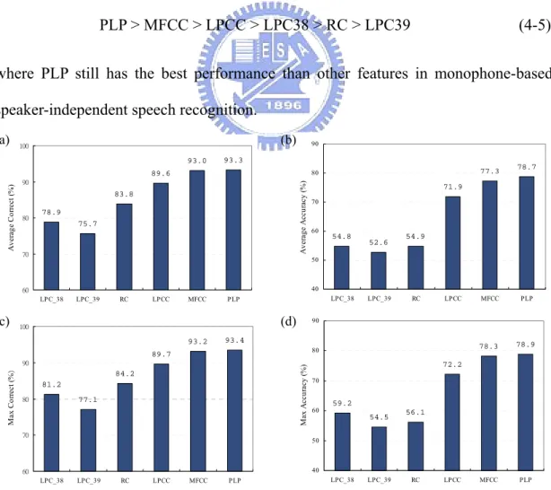
(9) Fig.3-5. Three-state left-to-right HMM with no skip ............................................. 34. Fig.3-6. Scheme of probability of the observations................................................ 36. Fig.3-7. (a) Speech labeled with the boundary and transcription save as text file (b) with and (c) without boundary information......................................... 38. Fig.3-8. Training procedure of the HMM ............................................................... 38. Fig.3-9. The block diagram of creating the initialized HMM................................. 41. Fig.3-10 Modified k-means ..................................................................................... 41 Fig.3-11 Maximization the probability of generating the observation sequence..... 42 Fig.4-1. HMM structure of (a) sp, (b) sil, (c) consonants and (d) vowels .............. 56. Fig.4-2. (a) HMM structure of the word “樂(l@4),” (b) “l” and (c) “@” .............. 56. Fig.4-3. Flow chart of training the monophone-based HMMs ............................... 58. Fig.4-4. 3-D view of the variations of the feature vectors (a) LPC-38 (b) LPC_39 (c) RC (d) LPCC (e) MFCC (f) PLP........................................... 59. Fig.4-5. Flow chart of testing the performance of different features...................... 60. Fig.4-6. Comparison of the different features (a) Correct (%) (b) Accuracy (%)... 62. Fig.4-7. Monophone-based HMM experiment (a) Average Correct (%) (b) Average Accuracy (%) (c) Max Correct (%) (d) Max Accuracy (%)........ 63. Fig.4-8. Flow chart of training the syllable-based HMMs...................................... 66. Fig.4-9. Flow chart of testing the syllable-based HMMs ....................................... 67. Fig.4-10. Comparison of the different features (a) Correct (%) (b) Accuracy (%)... 68. Fig.4-11. syllable-based HMM experiment (a) Average Correct (%) (b) Average Accuracy (%) (c) Max Correct (%) (d) Max Accuracy (%) ...................... 69. vii.

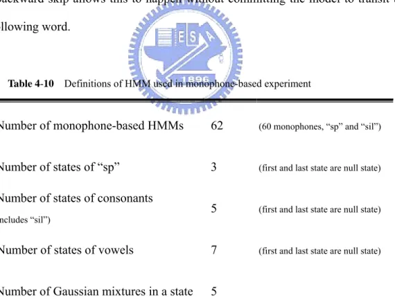
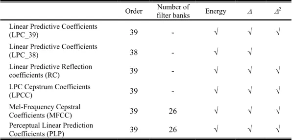
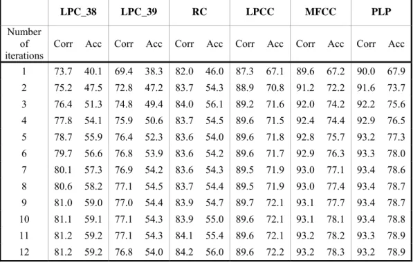
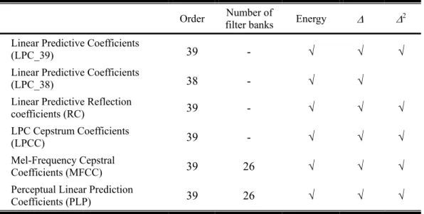
(10) Index of Tables Table 4-1. The recording environment of the TCC-300 corpus produced by NCTU..................................................................................................... 50. Table 4-2. The statistics of the database TCC-300 (NCTU) .................................. 50. Table 4-3. Recording environment of the connected-digits ................................... 51. Table 4-4. Statistics of the connected-digits database ............................................ 51. Table 4-5. The comparison table of 21 consonants of Chinese syllables between SAMPA-T and Chinese phonetic alphabets ............................ 52. Table 4-6. Comparison table of 39 vowels of Chinese syllables between SAMPA-T, and Chinese phonetic alphabets .......................................... 53. Table 4-7. A paragraph marked with Chinese phonetic alphabets ......................... 54. Table 4-8. Word-level transcriptions using SAMPA-T .......................................... 54. Table 4-9. Phone-level transcriptions using SAMPA-T ......................................... 54. Table 4-10 Definitions of HMM used in monophone-based experiment................ 55 Table 4-11 The parameters of front-end processing................................................ 57 Table 4-12 Six different features adopted in this thesis .......................................... 57 Table 4-13 Comparison of the Corr (%) and Acc (%) of different features ............ 61 Table 4-14 Definition of Hidden Markov Models used in syllable-based experiment ............................................................................................. 64 Table 4-15 Six different features adopted in this thesis .......................................... 66 Table 4-16 Comparison of the Corr (%) and Acc (%) of different features ............ 67 Table 5- 1 Performance Comparison Table ..............................................................71. viii.

(11) Chapter 1 Introduction. 1.1 Motivation Imaging that if we can control the equipments and tools in our surroundings through voice command, just like people in the sci-fi movies do, the world will be more convenient and fantastic. In many real-world applications, such as toys, cell phones, automatic ticket booking, goods ordering, etc and it can be foreseen that there will be more and more services provided in the form of speech in the future. The speaker-independent (SI) automatic speech recognition is the way to achieve the goal. Although the speaker-dependent automatic speech recognition system outperforms the speaker-independent automatic speech recognition system in the recognition rate, it is infeasible to collect large speech data of the user and then train the models in real applications, especially the popular commodities. Hence, the solution of providing services for general users is to build a speaker-independent (SI) automatic speech recognition system. It has been shown that the selection of parametric representations significantly affects the recognition results in an isolated-word recognition system [16]. Therefore, this thesis focuses on the selection of the best parametric representation of speech data for speaker-independent automatic speech recognition. The parametric representation, namely the feature extraction techniques, evaluated in this thesis can be divided into two groups: based on the speech production and based on the speech perception. The first group includes the Linear Predictive Coding (LPC), LPC-derived Cepstrum (LPCC) and Reflection coefficients (RC). The second group comprises the. 1.

(12) Mel-frequency Cepstral Coefficients (MFCC) and Perceptual Linear Predictive (PLP) analysis. In general, the speech signal is comprised of the context information and the speaker. information.. The. objective. of. selecting. the. best. features. of. speaker-independent automatic speech recognition is to eliminating the difference between speakers and enhancing the difference of phonetic characteristics. Therefore, in this thesis, two corpora are employed in the experiment to evaluate the performance of different features. In recent years, Hidden Markov Model (HMM) has become the most powerful and popular speech model used in ASR due to its remarkable ability of characterizing the acoustic signals in a mathematically tractable way and better performance compared to other methods, such as Neural Network (NN), Dynamic Time Warping (DTW). The statistical model HMM plays an important role to model the speech signals especially for speech recognition system since the template method is no more feasible for large number of users and large vocabulary system. HMM is proceeded after the extracting the features from the speech signal where the features means MFCCs, LPCs, PLPs, etc. The Hidden Markov Model is employed to model the acoustic features in all the experiments in this thesis.. 1.2 Overview The chapter of thesis is organized as follows. In chapter 2, the front-end techniques of the speech recognition system will be introduced, including the feature extraction methods, such as LPC, MFCC and PLP, utilized in this thesis. The chapter 3 will show the concept of Hidden Markov Model and its training and recognition procedure. Then the experimental results and comparison of different features will be shown in chapter 4. The experimental conclusion will be given in the last chapter.. 2.

(13) Chapter 2 Front-End Techniques of Speech Recognition System In modern speech recognition systems, the front-end techniques mainly includes converting the analog signal to a digital form, extracting important signal characteristics such as energy or frequency response, and augmenting perceptual meanings of these characteristics, such as human production and hearing. The purpose of the front-end processing of the speech signal is to transform a speech waveform into a sequence of parameter blocks and to produce a compact and meaningful representation of the speech signal. Besides, the front-end techniques can also remove the redundancies of the speech and then reduce the computational complexity and storage in the training and recognition steps, thus the performance of recognition will improve through effective front-end techniques. Independent of what the parameter kind extracted later is, there are four simple pre-processing steps, including constant bias removing, pre-emphasis, frame blocking, and windowing, which are applied prior to performing feature extraction. And these steps will be expressed and stated in the following four sections. In addition, three common feature extraction methods, Linear Prediction Coding (LPC) [2], Mel Frequency Cepstral Coefficient (MFCC) [3], and Perceptual Linear Predictive (PLP) Analysis [4], will be described in the last section of this chapter.. 2.1 Constant bias Removing The speech waveform probably has a nonzero mean, denoted as DC bias, due to the environments, the recording equipments, or the analogous-digital conversion. In. 3.

(14) order to get better feature vectors, it is necessary to estimate the DC bias and then remove it. The DC bias value is estimated by. DCbias =. 1 N ∑ s(k ) N k =1. (2-1). where s(k) is the speech signal possessing N samples. Then the signal after removing the DC bias, denoted by s ′(k ) , is given s ′(k ) = s (k ) − DC bias ,. 1≤ k ≤ N. (2-2). where N is the total samples of the speech signal. After the process of constant bias removing, the pre-emphasis filter is then applied to the speech signal s ′(k ) which is stated in the next section.. 2.2 Pre-emphasis The purpose of pre-emphasis is to eliminate the effect of glottis while producing sound and to compensate the high-frequency parts depressed by the speech generation system. Typically, the pre-emphasis is fulfilled with a high-pass filter in a form as P( z ) = 1 − µz −1 ,. 0.9 ≤ µ ≤1.0. (2-3). which increases the relative energy of the high-frequency spectrum and introduces a zero near µ. In order to cancel a pole near z = 1 due to the glottal effect, the value of µ is usually greater than 0.9 and it is set to be µ = 0.97 in this paper. The pole and zero −1. of the filter P(z) = 1- 0.97 z are 0 and 0.97 respectively. Furthermore, the frequency responses for the pre-emphasis filter with µ = 0.9, 0.97, and 1 are given in Fig 2-1. The filter is intended to boost the signal spectrum 20dB per decade approximately [5]. Fig.2-2 shows the comparison of the speech signal before and after pre-emphasis.. 4.

(15) Fig.2- 1 Frequency Response of the pre-emphasis filter. (a). (b). Fig.2- 2 Speech signal (a) before pre-emphasis and (b) after pre-emphasis. 2.3 Frame Blocking The objective of frame blocking is to decompose the speech signal into a series of overlapping frames. In general, the speech signal changes rapidly in time domain; 5.

(16) nevertheless, the spectrum changes slowly with time from the viewpoint of the frequency domain. Hence, it could be assumed that the spectrum of the speech signal is stationary in a short time, and then it is more reasonable to do spectrum analysis after blocking the speech signal into frames. There are two parameters should be concerned, that is frame duration and frame period, shown in Fig.2-3. I. Frame duration The frame duration is the length of time (in seconds), usually ranging between 10 ms ~ 30 ms, over which a set of parameters are valid. If the sampling frequency of the waveform is 16 kHz and the frame duration is 25 ms, there are 16 kHz × 25 ms = 400 samples in one frame. It is noted that the total number of samples in a frame is called the frame size. II. Frame period As shown in Fig.2-3, the frame period is often selected on purpose shorter than the frame duration to avoid the characteristics changing too rapidly between two successive frames. In other words, there is an overlap with time length equal to the difference of frame duration and frame period.. Frame 1. Frame n. Frame 2 Frame 3. ‧‧‧ ‧‧‧. Frame duration. Frame period. Feature vectors. ‧‧‧. Fig.2- 3 Frame blocking 6. ‧‧‧.

(17) 2.4 Windowing After frame blocking, the process of windowing applies to each frame by multiplying a Hamming window, shown in Fig.2-4 for N=64, to minimize the spectrum distortion and discontinuities. Let the Hamming window be given as ⎛ 2π n ⎞ w(n ) = 0.54 − 0.46 ⋅ cos⎜ ⎟, ⎝ N −1⎠. 0 ≤ n ≤ N−1. (2-4). where N is the window size, chosen the same as the frame size. Then the result of windowing process to m-th sample sm(n) can be obtained as smw (n ) = sm (n ) w(n ) ,. 0 ≤ n ≤ N−1. (2-5). Fig.2-5 shows an example of the time domain and frequency response for two successive frames, frame m and frame m+1, of the speech signal before and after multiplying by a Hamming window. From this figure, the spectrum of smw(n) is smoother than the sm(n). It is noted that there is little variation between two consecutive frames in their frequency response.. (a). (b). Fig.2- 4 Hamming window (a) in time domain and (b) frequency response. 7.

(18) frame m frame m+1. ……. windowing. windowing. smw(n). Fig.2- 5 Successive frames before and after windowing. 8.

(19) 2.5 Feature Extraction Methods Feature extraction is the major part of front-end technique for the speech recognition system. The purpose of feature extraction is to convert the speech waveform to a series of feature vectors for further analysis and processing. Up to now, several feasible features have been developed and applied to the speech recognition, such as Linear Prediction Coding (LPC), Mel Frequency Cepstral Coefficient (MFCC), and Perceptual Linear Predictive (PLP) Analysis, etc. The following sections will present all the techniques.. 2.5.1 Linear Prediction Coding (LPC). For the past years, Linear Prediction Coding (LPC), also known as auto-regressive (AR) modeling, has been regarded as one of the most effective techniques for speech analysis. The basic principle of LPC states that the vocal tract transfer function can be modeled by an all-pole filter as H (z ) =. S (z ) = GU ( z ). 1 p. 1 − ∑ ak z. = −k. 1 A( z ). (2-6). k =1. where S(z) is the speech signal, U(z) is the normalized excitation, G is the gain of the excitation, and p is the number of poles (or the order of LPC). As for the coefficients {a1, a2,…,ap}, they are controlled by the vocal tract characteristics of the sound being produced. It is noted that the vocal tract is a non-uniform acoustic tube which extends from the glottis to the lips and varies in shape as a function of time. Suppose that characteristic of vocal tract changes slowly with time, thus {ak} are assumed to be constant in a short time. The speech signal s(n) can be viewed as the output of the all-pole filter H(z), which is excited by acoustic sources, either impulse train with period P for voiced sound or random noise with a flat spectrum for unvoiced sound,. 9.

(20) shown in Fig.2-6. P Periodic impulses (voiced). P. U(z). Random noises (unvoiced). 1 H(z)= A( z ). S(z). G vocal tract model. glottis. Fig.2- 6 Speech production model estimated based on LPC model. From (2-6), the relation between speech signal s(n) and the scaled excitation Gu(n) can be rewritten as p. s (n ) = ∑ ak s (n − k ) + Gu (n ). (2-7). k =1. p. where. ∑ a s(n− k ) k =1. k. is a linear combination of the past p speech samples. In general,. the prediction value of the speech signal s(n) is defined as p. ˆs (n ) = ∑ ak s(n − k ). (2-8). k =1. and then the prediction error e(n) could be found as p. e(n ) = s(n ) − ˆs (n ) = s (n ) − ∑ ak s (n − k ). (2-9). k =1. which is clearly equal to the scaled excitation Gu(n) from (2-7). In other words, the prediction error reflects the effect caused by the scaled excitation Gu(n). To use the LPC is mainly to determine the coefficients {a1, a2,…,ap} that minimizes the square of the prediction error. From (2-9), the mean-square error, called the short-term prediction error, is then defined as En =. N −1+ p. ∑. m=0. en (m ) = 2. N −1+ p. ∑. m=0. p ⎛ ⎞ ⎜⎜ sn (m ) − ∑ ak sn (m− k )⎟⎟ k =1 ⎝ ⎠. 2. (2-10). where N is the number of samples in a frame. It is commented that the short-term. 10.

(21) 2. prediction error is equal to G and the notation of sn(m) is defined as ⎧s (m+ n ) w(m ), 0 ≤ m ≤ N − 1 sn (m ) = ⎨ otherwise ⎩0,. (2-11). which means sn(m) is zero outside the window w(m). It can be imaged that In the range of m = 0 to m = p − 1 or in the range of m = N to m = N − 1 + p , the windowed signals sn(m) are predicted as ŝn(m) by previous p signals and some of the previous signals are equal to zero since sn(m) is zero when m < 0 or m > N − 1 . Therefore, the prediction error en(m) is sometimes large at the beginning (m = 0 to m = p − 1 ) or the end ( m = N to m = N − 1 + p ) of the section (m = 0 to m = N − 1 + p ) . The minimum of the prediction error can be obtained by differentiating En with respect to each ak and setting the result to zero as ∂ En =0, ∂ ak. k = 1,2,..., p. (2-12). and then En is replaced by (2-11), the above equation can be rewritten as N −1+ p. ∑. m=0. p ⎞ ⎛ ⎜⎜ sn (m ) − ∑ aˆk sn (m− k )⎟⎟ sn (m− i ) = 0 , k =1 ⎠ ⎝. i = 1,2,..., p. (2-13). where i and k are two independent variables and aˆk are the values of ak for k = 1,2,…, p that minimize En. From (2-13), we can further expand the equation as N −1+ p. p. N −1+ p. m=0. k =1. m=0. ∑ sn (m ) sn (m− i ) = ∑ aˆk. where the term. ∑ s (m− k ) s (m− i ) ,. N −1+ p. N −1+ p. m=0. m=0. ∑ sn (m) sn (m− i ) and. n. n. ∑ s (m− k ) s (m− i ) n. n. i = 1,2,..., p. (2-14). will be replaced by the. autocorrelation function rn(i) and rn(i− k) respectively. The autocorrelation function is defined as rn (i − k ) =. N −1+ p. ∑ s (m− k ) s (m− i ) ,. m =0. n. n. 11. i = 1,2,..., p. (2-15).

(22) where rn(i− k) is equal to rn(k − i ). Hence, it is equivalent to use rn(|i− k|) to replace N −1+ p. the term. ∑ s (m− k ) s (m− i ). m=0. n. n. in (2-16). By replacing (2-16) with autocorrelation. function rn(i) and rn(i− k), we can obtain p. ∑ aˆ r ( i − k ) = r (i ) , k =1. i = 1,2,..., p. n. k n. (2-16). which matrix form is expressed as rn (1) rn (2 ) ⎡ rn (0 ) ⎢ r (1) rn (0 ) rn (1) ⎢ n ⎢ rn (2 ) rn (1) rn (0 ) ⎢ M M ⎢ M ⎢rn ( p − 2 ) rn ( p − 3) rn ( p − 4 ) ⎢ ⎣⎢ rn ( p − 1) rn ( p − 2 ) rn ( p − 3). L rn ( p − 2 ) rn ( p − 1) ⎤ ⎡ aˆ1 ⎤ ⎡ rn (1) ⎤ ⎢ ⎥ L rn ( p − 3) rn ( p − 2 )⎥⎥ ⎢ aˆ2 ⎥ ⎢⎢ rn (2 ) ⎥⎥ L rn ( p − 4 ) rn ( p − 3)⎥ ⎢ aˆ3 ⎥ ⎢ rn (3) ⎥ ⎥=⎢ ⎥⎢ ⎥ O M M ⎥⎢ M ⎥ ⎢ M ⎥ rn (0 ) rn (1) ⎥ ⎢aˆ p −1 ⎥ ⎢rn ( p − 1)⎥ L ⎥ ⎢ ⎥⎢ ⎥ rn (1) rn (0 ) ⎦⎥ ⎣⎢ aˆ p ⎦⎥ ⎣⎢ rn ( p ) ⎦⎥ L. (2-17). which is in the form of Rx = r where R is a Toeplitz matrix, that means the matrix has constant entries along its diagonal. The Levinson-Durbin recursion is an efficient algorithm to deal with this kind of equation, where the matrix R is a Toeplitz matrix and furthermore it is symmetric. Hence the Levinson-Durbin recursion is then employed to solve (2-20), and the recursion can be divided into three steps, as Step 1. Initialization E (0) = rn (0) , a (0 ,0 ) = 1 Step 2. Iteration ( aij is denoted as a ( i , j ) ) for i = 1 to p { i −1. k (i ) =. rn (i + 1) − ∑ a( j,i − 1) rn (i − j ) j =1. E (i − 1). a (i,i ) = k (i ). for j = 1 to i − 1. 12.

(23) a ( j,i ) = a ( j,i − 1) − k (i ) a (i − j,i − 1). (. ). E (i ) = 1 − k (i ) E (i − 1) 2. } Step 3. Final Solution for j = 1 to p a ( j ) = a ( j, p ). where the aˆ j = a( j ) for j = 1 , 2 , … , p , and the coefficients k ( i ) are called reflection coefficients whose value is bounded between 1 and -1. In general, the rn( i ) is replaced by a normalized form as rn_ normailizd (i ) =. rn (i ) rn (0). (2-18). which will result in identical LPC coefficients (PARCOR) but the recursion will be more robust to the problem with arithmetic precision. Another problem of LPC is to decide the order p. As p increases, more detailed properties of the speech spectrum will be reserved and the prediction errors will be lower relatively, but it should be notice when p is beyond some value that some irrelevant details will be involved. Therefore, the guideline for choosing the order p is given as ⎧ F + (4 or 5) p=⎨ s ⎩ Fs. voiced unvoiced. ,. (2-19). where Fs is the sampling frequency of the speech in kHz [6]. For example, if the speech signal is sampled at 8 kHz, then the order p is can be chosen as 8~13. Another rule of thumb is to use one complex pole per kHz plus 2-4 poles [7], hence p is often chosen as 10 for the sampling frequency 8 kHz. 13.

(24) Historically, LPC is first used directly in the feature extraction process of the automatic speech recognition system. LPC is widely used because it is fast and simple. In addition, LPC is effective to compute the feature vectors by Levinson-Durbin recursion. It is noted that the unvoiced speech has higher error than the voiced speech since the LPC model is more accurate for voiced speech. However, the LPC analysis approximates power distribution equally well at all frequencies of the analysis band which is inconsistent with human hearing because the spectral resolution decreases with frequency beyond 800 Hz and hearing is also more sensitive in the middle frequency range of the audible spectrum.[11] In order to make the LPC more robust, the cepstral processing, which is a kind of homomorphic transformation, is then employed to separate the source e(n) from the all-pole filter h(n). It is commented that the homomorphic transformation ˆx(n ) = D( x(n )) is a transformation that converts a convolution x(n ) = e(n ) ∗ h(n ). (2-20). ˆx(n ) = eˆ(n ) + hˆ(n ). (2-21). into a sum. which is usually used for processing signals that have been combined by convolution. It is assumed that a value N can be found such that the cepstrum of the filter hˆ(n ) ≈ 0 for n ≥ N and the excitation of eˆ(n ) ≈ 0 for n < N. The lifter (“l-i-f-ter” is the inverse of the word “f-i-l-ter”) l(n) is used for approximately recovering eˆ(n ) and hˆ(n ) from ˆx(n ) . Fig.2-7 shows how to recover h(n) with l(n) given by ⎧1 l (n ) = ⎨ ⎩0. n<N. (2-22). n≥N 14.

(25) -1. and the operator D usually uses the logarithmic arithmetic and D. use inverse. Z-transform. In the similar way, the l(n) is given by. ⎧1 l (n ) = ⎨ ⎩0. n≥N. (2-23). n<N. which is utilized for recovering the signal e(n) from x(n). In general, the complex cepstrum can be obtained directly from LPC coefficients by the formula expressed as ⎧0 ⎪ln G ⎪ n −1 ⎪ ⎛k⎞ hˆ(n ) = ⎨an + ∑ ⎜ ⎟ hˆ(k ) an − k ⎪ n −1 k =1 ⎝ n ⎠ ⎛k ⎞ˆ ⎪ ∑ ⎪k = n − p ⎜⎝ n ⎟⎠ h(k ) an − k ⎩. n<0 n=0 0<n≤ p. (2-24). n> p. where hˆ (n) is the desired LPC-derived cepstrum coefficients c(n). It is noted that, while there are finite number of LPC coefficients, the number of cepstrum is infinite. Empirically, the number of cepstrum which is approximately equal to 1.5p is sufficient.. x(n). D[. ˆx(n ). ]. hˆ(n ). l(n). -1. D [. Multiply ˆx (n ) by l(n). n ≈ hˆ(n ). N. ≈ eˆ(n ). N. Fig.2- 7 Homomorphic filtering. 15. ]. h(n).

(26) 2.5.2 Mel-Frequency Cepstral Coefficients (MFCC). The Mel-Frequency Cepstral Coefficients (MFCC) is the most widely used feature extraction method for state-of-the-art speech recognition system. The conception of MFCC is to use nonlinear frequency scale, which approximates the behavior of the auditory system. The scheme of the MFCC processing is shown in Fig.2.8, and each step will be described below.. {s(k)}. Pre-processing. {sw(k)}. FFT. {St(k)} Mel-Frequency. {Xt(m)}. Filter Banks. Speech Energy. logΣ Xt(m). et ct(i). derivatives. DCT. Yt (m). Mel Cepstrum c(i ), et ⎫ ⎧ ⎪ ⎪ { ( ) } { } yt = ⎨ ∆ c i , ∆ et ⎬ ⎪ ∆2 c(i ) , ∆2 e ⎪ t ⎭ ⎩. {. }{ }. Fig.2- 8 Scheme of obtaining Mel-frequency Cepstral Coefficients. After the pre-processing steps discussed above, including constant bias removing, pre-emphasis, frame blocking, and windowing, are applied to the speech signal, the Discrete Fourier Transform (DFT) is then performed to obtain the spectrum where DFT is expressed as N −1. St (k ) = ∑ sw (i )e − j 2π ik/N ,. 0≤k < N. (2-25). i =0. where N is the size of DFT chosen the same as the window size. The Fast Fourier Transform (FFT) is often adopted to substitute for the DFT for more efficient computation. The Mel filter banks will be defined later after making a short introduction of the Mel scale. 16.

(27) The Mel scale, is obtained by Stevens and Volkman [8][9], is a perceptual scale motivated by nonlinear properties of human hearing and it attempts to mimic the human ear in terms of the manner that the frequencies are sensed and resolved. In the experiment, the reference frequency was selected as 1 kHz and equaled it with 1000 mels where a mel is defined as a psychoacoustic unit of measuring for the perceived pitch of a tone [10]. The subjects were asked to change the frequency until the pitch they perceived was twice the reference, 10 times, half, 1/10, etc. For instance, if the frequency they perceived is twice the reference, namely 2 kHz, while the actual frequency is 3.5 kHz, the frequency 3.5 kHz is mapping to the Mel frequency twice 1000 mels, that is, 2000 mels. The formulation of Mel scale is approximated by f ⎞ ⎛ B( f ) = 2595 log10 ⎜1 + ⎟ ⎝ 700 ⎠. (2-26). where B ( f ) is a function for mapping the actual frequency to the Mel frequency, shown in Fig.2.9, and the Mel scale frequency is almost linear below 1 kHz and is logarithmic above. The Mel filter bank is then designed by placing M triangular filters non-uniformly along the frequency axis to simulate the band-pass filters of human ears, and the m-th triangular filter is expressed as 0 ⎧ ⎪ (k − f (m − 1)) ⎪ ⎪ ( f (m ) − f (m − 1)) H m (k ) = ⎨ ( f (m + 1) − k ) ⎪ ⎪ ( f (m + 1) − f (m )) ⎪⎩ 0. k < f (m − 1) f (m − 1) ≤ k ≤ f (m ) f (m ) ≤ k ≤ f (m + 1) k > f (m + 1). 0 ≤ k < N , 1≤ m ≤ M M. which satisfies. ∑ H (k ) = 1 m =1. m. ,. (2-27). and N is the size of the FFT. The boundary points f ( m ). in the above equation can be calculated by. 17.

(28) ⎛N⎞ ⎛ B( f h ) − B( f l ) ⎞ f (m ) = ⎜⎜ ⎟⎟ B −1 ⎜ B( f l ) + m ⎟, M +1 ⎠ ⎝ Fs ⎠ ⎝. 1≤ m ≤ M. (2-28). where fl and fh is the lowest and highest frequency (Hz) of the filter bank, Fs is the sampling frequency of the speech signal and the function B ( f ) is the function to map -1 the actual frequency to Mel frequency given in (2-24). The function B (b) is the. inverse of the B( f ) given by. (. ). B −1 (b ) = 700 10b/ 2295 − 1. (2-29). where b is the Mel frequency. It is noted that the boundary points f ( m ) are uniformly -1. spaced in the Mel scale. By replacing B and B in (2-28) by (2-26) and (2-29), the equation can be rewritten as m ⎤ ⎡ M ⎛ ⎞ 700 + f l 700 + f h + 1 700 ⎥ ⎢ ⎟⎟ ⋅ ⎜⎜ − f (m ) = N ⋅ ⎢ Fs + 700 f Fs ⎥ l ⎠ ⎝ ⎥⎦ ⎢⎣. (2-30). which can be used in programming. In general, M is equal to 20 for the speech signal with 8 kHz sampling frequency and 24 for 16 kHz sampling frequency. The Mel filter banks of the 8 kHz (M = 20) and 16 kHz (M = 24) are shown in Fig.2-10(a) and Fig.2-10(b) respectively. The region of spectrum below 1 kHz is processed by more filter banks since this region contains more information on the vocal tract such as the first formant. The nonlinear filter bank is employed to achieve both frequency and time resolution where the narrow band-pass filter at low frequencies enables harmonics to be detected and the longer band-pass filter at high frequencies allows for higher temporal resolution of bursts.. The Mel spectrum is derived by multiplied each FFT magnitude coefficient with the corresponding filter gain as 18.

(29) X t (k ) = St (k ) H m (k ) ,. 0 ≤ k < N−1. (2-31). and the results is accumulated and taken logarithm as N −1. Yt (m ) = log ∑ X t (k ) ,. 0≤m<M. (2-32). k =0. which is robust to noise and spectral estimation errors. The reason of using the magnitude of St(k) is that the information of phase is useless in speech recognition. The logarithm operation is utilized to reduce the component amplitudes at every frequency and to perform a dynamic compression in order to make the feature extraction less sensitive to variations in dynamics where the dynamics means the magnitude of the sound. Besides, the logarithm is applied to separate the excitation produced by the vocal tract and the filters that represents the vocal tract. Since the log-magnitude spectrum Y(m) is real and symmetric, the inverse Discrete Fourier Transform (IDFT) is reduced to the Discrete Cosine Transform (DCT) and applied to derive the Mel Frequency Cepstral Coefficients ct (i) as. ct (i ) =. 2 M. ⎛ iπ ⎛. M. 1 ⎞⎞. ∑ Y (m )cos⎜⎜⎝ M ⎜⎝ m− 2 ⎟⎠ ⎟⎟⎠ , m=1. i = 1,L , L. (2-33). where L is the number of cepstrum coefficients desired and L ≤ M . It is noted that the cepstrum is defined in the quefrency domain. The process of DCT successfully separates the excitation and the vocal tract, in other words, the low quefrencies, namely lower order of cepstrum, represents the slow changes of the envelope of the vocal tract and the high quefrencies, namely, higher order of cepstrum represents the periodic excitation. In general, 12 MFCCs (L=12) and the energy is adapted where the energy term computed by the log of the energy as N. et = log ∑ sw (k ). 2. (2-34). k =1. which often referred to as absolute MFCCs, and then the first and second-order. 19.

(30) derivatives of these absolute coefficients are given. ∑ p(c (i ) − c (i )) P. ∆ ct (i ) =. p =1. t+ p. t− p. P. 2∑ p. ,. 2. i = 1,L , L. (2-35). i = 1,L , L. (2-36). p =1. and. ∑ p(∆ c (i ) − ∆ c (i )) P. ∆ ct (i ) = 2. p =1. t+ p. t− p. P. 2∑ p. ,. 2. p =1. which are useful to cancel the channel effect of the speech. In addition, the derivative operation is utilized to obtain the dynamic evolution of the speech signal, that is, the temporal information of the feature vector ct (i). If the value of P is too small, the dynamic evolution may not be caught; if the value P is too large, the derivatives have less meaning since two frames may describe different acoustic phenomena. In practice, the order of MFCC is often chosen as 39, including 12 MFCCs ({c(i)}|i=1,2,…,12), energy term (et) and their first-order derivatives (∆{c(i)}|i=1,2,…,12, ∆{et}) and second-order derivatives (∆2{c(i)}|i=1,2,…,12, ∆2{et}). (a). (b). Fig.2- 9. Frequency Warping according to the Mel scale (a) linear frequency scale (b) logarithmic frequency scale. 20.

(31) (a). H1(k). ……. H18(k) H19(k) H20(k). H2(k). (b). H1(k) H2(k). ……. H22(k). H23(k) H24(k). Fig.2-10 The Mel filter banks (a) Fs = 8 kHz and (b) Fs =16 kHz. 2.5.3 Perceptual Linear Predictive (PLP) Analysis. The Perceptual Linear Predictive (PLP) analysis is first presented and examined by Hermansky in 1990 [4] for analyzing speech. This technique combines several engineering approximations of psychophysics of human hearing processes, including critical-band spectral resolution, the equal-loudness curve, and the intensity-loudness power law. As a result, the PLP analysis is more consistent with the human hearing. In addition, the PLP analysis is beneficial for speaker-independent speech recognition due to its computational efficiency and yielding a low-dimensional representation of 21.

(32) speech. The block diagram of the PLP method is shown in Fig.2.11, and each step will be described below. [12]. {s(k)}. Pre-processing. {sw(k)}. Critical-band. FFT. analysis. Speech. Equal-Loudness. Intensity-Loudness. Pre-emphasis. Conversion. Autoregressive modeling. Fig.2-11. IDFT. All-pole Model. Scheme of obtaining Perceptual Linear Predictive coefficeints. Step I. Spectral analysis The fast Fourier Transform (FFT) is first applied on the windowed speech segment (sw(k), for k=1,2,…N) into the frequency domain. The short- term power spectrum is expressed as P(ω ) = [Re(St (ω ))] + [Im(St (ω ))] 2. 2. (2-37). where the real and imaginary components of the short-term speech spectrum are squared and added. There is an example in Fig.2-12 which shows the short-term speech signal and its power spectrum P(ω).. 22.

(33) (a). (b). Fig.2-12 Short-term speech signal (a) in time domain and (b) power spectrum. Step II.. Critical-band analysis. The power spectrum P(ω) is then warped along the frequency axis ω into the Bark scale frequency Ω as 2 ⎧⎪ ω ⎫⎪ ⎛ ω ⎞ + + ⎜ 1 ⎟ ⎬ ⎝ 1200π ⎠ ⎪⎩1200π ⎪⎭. Ω (ω ) = 6ln ⎨. (2-38). where ω is the angular frequency in rad/sec, which is shown in Fig.2-13. The resulting power spectrum P(Ω ) is then convoluted with the simulated critical-band masking curve Ψ ( Ω ) and get the critical-band power spectrum Θ (Ω i ) as. Θ (Ω i ) =. 2.5. ∑ P(Ω )Ψ (Ω − Ω ) ,. Ω = −1.3. i. i = 1,2,..., M. (2-39). where M is number of Bark filter banks and the critical-band masking curve Ψ ( Ω ), shown in Fig.2-14, is given by,. 23.

(34) ⎧ ⎪ ⎪⎪ Ψ (Ω )= ⎨ ⎪ ⎪ ⎪⎩. 0 100.5( Ω + 0.5 ) 1 10−1.0( Ω − 0.5 ) 0. for for for for for. Ω < −1.3 − 1.3 ≤ Ω ≤ −0.5 − 0.5 < Ω < 0.5 0.5 ≤ Ω ≤ 2.5 Ω > 2.5. (2-40). where Ω is the Bark frequency just mentioned in (2-38). This step is similar to Mel filter banks processing of MFCC where the Mel filter banks are replaced by the analogous trapezoid Bark filter banks. The step between two banks is constant on the Bark scale, and the interval is chosen so that the filter banks must cover the whole analysis band. For example, 21 Bark filter banks, which cover from 0-Bark to 19.7-Bark in 0.985-Bark steps, are employed for analyzing speech signal of 16 kHz sampling frequency, shown in Fig.2-15. It is noted that 8 kHz is mapping to 19.687-Bark and the steps are usually chosen approximately 1-Bark. Fig.2-16 is the power spectrum after applying the Bark filter banks (M = 21) to the speech signal in Fig.2-12. The Bark filter banks and the Mel filter banks are both allocate more filters to the lower frequencies, where the hearing is more sensitive. Sometimes, the Bark filter banks are replaced with the Mel filter banks.. Fig.2-13 Frequency Warping according to the Bark scale. 24.

(35) Fig.2-14 Critical-band curve. Fig.2-15 The Bark filter banks (a) in Bark scale (b) in angular frequency scale. 25.

(36) Fig.2-16 Critical-band power spectrum. Step III.. Equal-loudness pre-emphasis. In order to compensate the unequal sensitivity of human hearing at different frequencies, the sampled power spectrum Θ ( Ω i ) obtained in the (2-39) is then pre-emphasis by the simulates equal loudness curve E(ω), expressed as. Ξ (Ω i ) = E (ω ) ⋅ Θ (Ω i ) ,. i = 1,2,..., M. (2-41). where the function E(ω) is given by. E(ω) =. (ω + 56.8 ×10 )ω (ω + 6.3×10 ) × (ω + 0.38×10 )× (ω 2. 2. 6 2. 6. 2. 4. 9. 6. + 9.58×1026. ). (2-42). where E(ω) is a high pass filter. Then the value of the first and last samples are made equal to the values of their nearest neighbors, thus Ξ ( Ω i ) begins and ends with two equal-valued samples. Fig.2-17 shows the power spectrum after equal-loudness pre-emphasis. From the Fig.2-17, the part of higher frequency in Fig.2-16 has been well compensated.. 26.

(37) Fig.2-17 Equal loudness pre-emphasis. Step IV. Intensity-loudness power law Since the nonlinear relation between intensity of the sound and its perceived loudness, the spectral compression is then utilized by using the power law of hearing given by. Φ (Ω i ) = Ξ (Ω i )0.33 ,. i = 1,2,..., M. (2-43). where a cubic root compensation of critical band energies is applied. This step can reduce the spectral-amplitude variation of the critical-band spectrum. It is noted that the log arithmetic is adopted in the process of MFCC.. Fig.2-18 Intensity-loudness power law. 27.

(38) Step V. Autoregressive modeling The autocorrelation coefficients rs(n) are not computed in the time domain through (2-18) but is obtained as the inverse Fourier transform (IDFT) of the power spectrum P(ω) of the signal. The IDFT is better choice than the FFT here since only a few autocorrelation values are needed. If the order of the all pole model is equal to p, only the first p+1 autocorrelation values are used to solve the Yule-Walker equation. Then the standard Durbin-Levinson recursion is employed to compute the PLP coefficients.. 28.

(39) Chapter 3 Speech Modeling and Recognition. During the past several years, Hidden Markov Model (HMM) [20][21][22] has become the most powerful and popular speech model used in ASR because of its wonderful ability of characterizing the speech signal in a mathematically tractable way and better performance comparing to other methods. The assumption of the HMM is that the data samples can be well characterized as a parametric random process, and the parameters of the stochastic process can be estimated in a precise and well-defined framework.. 3.1 Introduction In a typical HMM based ASR system, the HMM is proceeded after the feature extraction. The input of the HMM is the discrete time sequence of feature vectors, such as MFCCs, LPCs, etc. These feature vectors are customarily called observations, since these feature vectors represent the inforamtion observable from the incoming speech utterance. The observation sequence O ={ o1, o2, …, oT} is a set of the observations from time 1 to time T, where the time t is the frame index. An Hidden Markov Model can be used to represnent a word (one, two, three, etc) , a syllable (“grand”, “fa”, “ther”, etc), a phone (/b/, /o/, /i/, etc), and so forth. The Hidden Markov Model is essentially structured by a state sequence q = {q1 , q2 ,L , qT } where qt ∈ {S1 , S 2 ,L , S N } , N is the total number of states and each state is generally associated with a multidimensional probability distribution. The states of HMM can. 29.

(40) be viewed as collections of similar acoustical phenomena in an utterance. The total number of state N should be chosen well to represent these phenomena. In general, different number of state of HMM would lead to differnet recognition results [12].. For a particular state, an observation can be generated according to the associated probability distribution. This means that there is not a one-to-one correspondence between the observation and the state, and the state sequence cannot be determined unanimously by a given oberservation sequence. It is noticed that only the observation is visible, not the state. In other words, the model possesses hidden states and is named as the “Hidden” Markov Model.. 3.2 Hidden Markov Model Formally speaking, a Hidden Markov Model is defined as Λ = ( A, B ,π ) , which includes the initial state distribution π, state-transition probability distribution A, and observation probability distribution B. Each elements will be illustrated respectively as follows. I. Initial state distribution π The initial state distribution is defined as π = { π i }in which. π i = P(q1 = Si ) ,. 1≤ i ≤ N. (3-1). where π i is the probability that the initial state q1 of the state sequence q = {q1 , q2 ,L , qT } is Si. Thus, the summation of the probability of all possible initial. state is equal to 1, given as. π1 + π 2 + L + π N = 1. (3-2). 30.

(41) II. State-transition probability distibution A The state transition probability distribution A of an N-state HMM can be expressed as { aij} or in the form of square matrix ⎡ a11 a12 ⎢a a22 A = ⎢ 21 ⎢ M M ⎢ ⎣a N 1 aN 2. L a1 N ⎤ L a2 N ⎥⎥ O M ⎥ ⎥ L aNN ⎦. (3-3). with constant probability aij. aij = p(qt +1 = j | qt = i ) ,. 1 ≤ i, j ≤ N. (3-4). representing the transition probability from state i at time t to state j at time t +1. Briefly, the transitions among the states are governed by a set of probabilities aij, called the transition probabilities, which are assumed not changing with time. It is noticed that the summation of all the probabilities from a particular state at time t to itself and the others at time t +1 should be equal to 1, i.e. the summation of all the entries in the i-th row is equal to 1, given as. ai 1 + ai 2 + L + aiN = 1 ,. i = 1,2,..., N. (3-5). For any state sequence q = {q1 , q2 ,L , qT } where qt ∈ {S1 , S 2 ,L , S N }, the probability of q being generated by the HMM is. P(q | A,π ) = π i aq1 q 2 aq 2 q3 L aqT −1qT. (3-6). For example, the transition probability matrix of a three-state HMM can be expressed in the form as ⎡ a11 a12 A = ⎢⎢a21 a22 ⎢⎣ a31 a32. a13 ⎤ a23 ⎥⎥ a33 ⎥⎦. (3-7). where 31.

(42) ai 1 + ai 2 + ai 3 = 1 ,. i = 1,2,3. (3-8). for arbitrary time t. Fig.3-1 shows all the possible paths, labeled with transition probabilities between states, from time 1 to T. The structure without any constrain imposed on state transitions is called ergodic HMM. It is easy to find that the number. ( ). of all possible paths N 2. T −1. (in this case N = 3 ) would greatly increase as time. increasing. q1. q2. state. a11. S1. π1. a13. π2. a21 S2. S1. qT-1. ‧‧‧. a21 S2. ‧‧‧. S2. a31 S3. S1. a12. a13. a23. π3. a11. S1. a12. a22. qT. a22. S2. a23 a31. a32 a33. 1. S3. ‧‧‧. 2 Fig.3-1. S3. T-1. a32 a33. S3. T. Time. Three-state HMM. A left-to-right HMM (namely Bakis model) with the elements of the state-transition probability matrix. aij = 0 ,. for j < i. (3-9). is adopted in general cases to simplify the model and reduce the computation time. The main conception of a left-to-right HMM is that the speech signal varies with time from left to right, that is, the acoustic phenomena change sequentially and the first state must be S1. There are two general types of left-to-right HMM, shown in Fig.3-2.. 32.

(43) By using a three-state HMM as an example, the transition probability matrix A with left-to-right and one-skip constrain, shown in Fig.3-3, can be express as ⎡a11 a12 A = ⎢⎢ 0 a22 ⎢⎣ 0 0. a13 ⎤ a23 ⎥⎥ a33 ⎥⎦. (3-10). where A is an upper-triangular matrix with a21 = a31 = a32 = 0. Fig.3-4 shows all possible paths between states of a three-state left-to-right HMM from time 1 to time T. If no skip is allowed, the transition probability matrix A can be express as ⎡a11 a12 A = ⎢⎢ 0 a22 ⎢⎣ 0 0. 0⎤ a23 ⎥⎥ a33 ⎥⎦. (3-11). where the element a13 in (3-7) is replaced by zero. Similarly, Fig.3-5 shows all possible paths between states of a no-skip three-state HMM from time 1 to time T.. (a). (b). Fig.3-2. Four-state left-to-right HMM with (a) one skip and (b) no skip. a23. a12 S1. a33. a22. a11. S2 a13 Fig.3-3 Typical left-to-right HMM with three states. 33. S3.

(44) state S1. a11. S1. ‧‧‧. a12. a13 S2. S2. a11. S1. ‧‧‧. a22. S2. S1. a12. S2. a23. S3. a33. 1 Fig.3-4. state S1. S3. ‧‧‧. 2. S3. a33. T-1. T. Time. Three-state left-to-right HMM with one skip. a11. S1. ‧‧‧. a11. S1. a12. S2. S3. S1. a12. S2. ‧‧‧. a22. S2. S2. a23. S3. S3. S3. 1. 2. T-1. Fig.3-5. a33. S3. T. Time. Three-state left-to-right HMM with no skip. III. Observation probability distribution B Since the state sequence q is not observable, each observation ot can be envisioned as being produced with the system in state qt . Assume that the production of ot in each possible state Si is stochastic, where i =1, 2,…, N, and is characterized by a set of observation probability functions B = {bj(ot)} where. b j (ot ) = P (ot | qt = S j ) ,. j = 1,2,..., N 34. (3-12).

(45) which discribes the probability of the observation ot being produced with respect to state j. If the distribution of the observations are continuous and infinite, the finite mixture of Gaussian distributions, that is, a weighted sum of M Gaussian distributions is used, expressed as. b j (ot ) = ∑ w j mN (µ jm , Σ jm ,ot ) M. m=1. ⎡ M = ∑ w jk ⎢ ⎢ m =1 ⎣. (. 1. 2π. ). L. Σ jm. 1 2. ⎤ ⎛ 1 ⎞ T −1 exp⎜ − (ot − µ jm ) Σ jm (ot − µ jm )⎟⎥ ⎝ 2 ⎠⎥ ⎦. (3-13). where µ jm and Σ jm indicates the mean vector and the covariance matrix of the m-th mixture component in state Sj. The observations are assumed to be independent to each other, the covariance matrix can be reduced to a diagonal form Σ jm as. Σ jm. 0 ⎡σ jm (1) ⎢ 0 σ jm (2) =⎢ ⎢ M M ⎢ 0 ⎣⎢ 0. ⎤ L 0 ⎥⎥ O M ⎥ ⎥ L σ jm (L )⎦⎥. L. 0. (3-14). or simplified as a vector with L-dimension as. [. ]. Σ jk = σ jk (1) σ jk (2 ) L σ jk (L ). (3-15). where L is the dimension of the observation ot. The mean vector can be expressed as. [. ]. µ jm = µ jm (1) µ jm (2 ) L µ jm (L ). (3-16). Then, the observation probability function bj(ot) can be written as ⎡ ⎢ M ⎢ 1 b j (ot ) = ∑ w jm ⎢ 1 m =1 L⎡ L ⎢ ⎤2 ⎢ (2π ) 2 ⎢∏ σ jm (l )⎥ ⎣ l =1 ⎦ ⎣. ⎤ ⎥ L ⎛ (ot (l ) − µ jm (l ))2 ⎞⎥ ⎟⎥ (3-17) exp⎜ − ∏ ⎜ ⎟ ( ) 2 σ l l =1 jm ⎝ ⎠⎥ ⎥ ⎦. As for the weighting coefficient w jk, it must satisfying M. ∑w m =1. jm. =1. (3-18) 35.

(46) where wjk is non-negative value. Fig.3-6 shows that the probabilities of the observations sequence O ={o1, o2, o3,. o4 } generated by state sequence q = {q1, q2, q3, q4} are bq1(o1), bq2(o2), bq3(o3), bq4(o4), respectively.. aq1 q2. q1. aq2 q3. …. bq (o2). …. q2. bq (o1) 1. qT-1. o2. qT. bq (oT-1). 2. o1. aqT-1 qT. bq (oT). T-1. …. oT-1. T. oT. …. Observations. Fig.3-6. time. Scheme of probability of the observations. 3.3 Training Procedure Given a HMM Λ ={ A, B, π } and a set of observations O ={o1, o2,…, oT }, the purpose of training the HMMs is to adjust the model parameters so that the likelihood P (O | Λ ) is locally maximized by using iterative procedure. The modified k-means. algorithm [19] and Viterbi algorithm are employed in the process of obtaing initial HMMs. The Baum-Welch algorithm (or called the forward-backward algorithm) is performed to train the HMMs. Before applying the training algorithm, prepareation work of the corpus and HMM is required prior to the trainging procedure as below I. A set of speech data and their associated transcriptions should be prepared, and the speech data must be transformed to the a series of feature vectors (LPC, RC, LPCC, MFCC, PLP, etc). 36.

(47) II. The number of states and the number of mixtures in a HMM must be determined, according to the degree of variations in the unit. In general, 3~5 states and 6~8 states are used for representing the English phone and Mardarin Chinese phone, respectively. It is noted that the features are the the observations of the HMM, and these observations and the transcriptions are then utilized to train the HMMs. The training procedure can be divided into two manners depending on whether the sub-word-level segment information, or called the boundary information, is available, that is labeled with boundary manually. If the segment information is available, such as Fig.3-7(a), the estimation of the HMM parameter would be easier and more precise; otherwise, training with no segment information would cost more computation time to re-align the boundary and re-estimate the HMM, in addition, the HMM often performs not as good as the one with well-segment information. The transcription and boundary condition should be saved in text files, such as the form in Fig.3-7(b)(c). It is noted that if the speech doesn’t have segment information, it is also necessary to get the transcription and save it before training. The block diagram of the training procedure is shown in Fig.3-8. The main difference between training the HMM with boundary information and training the HMM without boundary information is on the processing of creating the initialized HMM. Then, the following section will divided into two parts to present the details of creating the initialized HMM. (a). 37.

(48) (b). (c) 0 60 sil. sil. 60 360 yi. yi. 360 370 sp. sp. 370 600 ling. ling. 600 610 sp. sp. 620 1050 wu. wu. 1050 1150 sil. sil. Fig.3-7 (a) Speech labeled with the boundary and transcription save as text file (b) with and (c) without boundary information. … Feature vectors (observations). With boundary information?. No. Yes. Initial HMM with k-means and Viterbi alignment (Fig.3-9). Initial HMM with global mean and variance. Baum-Welch and Viterbi alignment to obtain estimated HMM. Viterbi search. Baum-Welch re-estimation. Baum-Welch re-estimation. Get HMMs. Get HMMs. Fig.3-8. Training procedure of the HMM 38.

(49) I. Boundary information is available The procedure of creating the initialized HMMs is shown in Fig.3-9, Fig 3-10. The modified k-means algorithm and the viterbi algorithm are utilized in training iteration. On the first iteration, the training data of a specific model are uniformly divided into N segments, where N is the number of states of HMM, and the successive segments are associated with successive states. Then, the HMM parameters πi and aij can be estimated first by. πj =. number of observations in state j at time = 1 number of observations at time = 1. (3-19). aij =. number of transitions from state i to state j number of transitions from state i. (3-20). 3.3.1 Midified k-means algorithm. For continuous-density HMM with M Gaussian mixtures per state, the modified k-means [13][14] are used for cluster the observations O into a set of M clusters which are associated to the number of mixtures in a state, shown in Fig.3-9. Let the i-th cluster of a m-cluster set at the k-th iteration denote as ω m,k i where i =1,2,…, m and k = 1,2,…, k max with kmax being the maximum allowable iteration count. Y(ω) is the representive pattern for cluster ω. the number of clusters in the current iteration and i is the iteration counter in classification process. The modified k-means algorithm is given by (i). Set m=1, k =1 and i =1; ωm,k i = O and compute the mean Y(Ο) of the entire training set O.. (ii) Classify the vectors by minimum distance principle. Accumulate the total 39.

(50) intracluster distance for each cluster ωm,k i denoted as ∆ik . If none of the following conditions meet then back to (ii) and k = k+1. a. ωm,k +1i = ωm,k i , for all i=1,2,…,m b. k meets the preset maximum allowable number of iterations. c. The change in the total accumulated distance is below the preset threshold ∆th . (iii) Record the mean and the covariance of the m-cluster,. If m is reached the number of mixtures M, then stop, else, go to (iv). (iv) Split the mean of the cluster that has largest intracluster distance and m=m+1, reset k and go to (ii).. From the modified k-means, the observations are clustered into M groups where M is the number of mixtures in a state. The parameters can be estimated by w jm =. N number of observations classified in cluster m in state j = jm Nj number of observations classified in state j. (3-21). N. µ jm. jm 1 ⋅ ∑ on (3-22) = mean of the observations classifiedin cluster m in state j = N jm n =1. Σ jm = covariance matrix of the observations classified in cluster m in state j N. jm 1 ˆ j m )(on − µ ˆ jm )T = ⋅ ∑ (on − µ N jm n =1. (3-23). where on (1≤ n ≤ Njm ) is the observations classified in cluster m in state j. Then the HMM parameters is all updated.. 40.

(51) … Viterbi alignment. Feature vectors (observations). Uniform Segmentation Modified k-means Modified k-means Update the Model parameters Initialize Parameters Converged ?. Initialized HMM Fig.3-9. The block diagram of creating the initialized HMM. q1. …. q2. bq (o1). …. bq (o2). 1. bq (oT-1). …. o2. bq (oT). T-1. 2. o1. qT. qT-1. T. oT-1. oT. …. Cluster 1. ×. ×. ××. 。. Global mean. ×. × × ×× × × × ×。 × × ×. ×. ×. ×. Cluster 2. ×× ×. × × ×. × ×. ×. ×. ××. ×. ×. ××. × × ×. ×. 。. 。 × ×. ×. Cluster 2. × × × × × × ×× ×. {ω13, µ13, Σ13} Cluster 3. Fig.3-10 Modified k-means. 41. {ω11, µ11, Σ11} Cluster 1 {ω , µ , Σ } 12 12 12.

(52) 3.3.2 Viterbi Search. Except for the first estimation of the HMM, the uniform segmentation is replaced by Viterbi alignment, viz Viterbi search, which is applied to find the optimal state sequence q ={q1, q2,…,qT} where model Λ and the observations sequences O ={o1, o2,…, oT } are given. By the Viterbi alignment, each observation will be. re-align to the state so that the new sate sequence q ={q1, q2,…,qT} maximizes the probability of generating the observation sequence O ={o1, o2,…, oT }. By taking logarithm of the model parameters, the Viterbi algorithm [14] can be impletement with only N T additions and wihout any multiplications. Define δ t (i ) 2. be the highest probability along the singal path at time t, expressed as. δ t (i ) =. max. q = {q1 ,q 2 , ,...,q t −1 }. P (q1 ,q2 , ,...,qt −1 ,qt = i, o1 ,o2 , ,...,ot | Λ). (3-24). and by induction we can obtain. [. ]. δ t +1 ( j ) = max δ t (i ) aij b j (ot +1 ) i. (3-25). which is shown in Fig.3-11.. state. ‧‧‧. δt (1). a11. S1. a12 ‧‧‧. δt (2). a22. S2. a23 ‧‧‧. δt (3). a33. S3. t Fig.3-11. b1(ot+1) S1. ‧‧‧. b2(ot+1) S2. ‧‧‧. b3(ot+1) S3. t+1. ‧‧‧ time. Maximization the probability of generating the observation sequence 42.

(53) The Viterbi algorithm is expressed as follows (i) Preprocessing. π~i = log(π i ) ,. 1≤ i ≤ N. (3-26). ~ bi (ot ) = log(bi (ot )) ,. 1≤ i ≤ N , 1≤ t ≤ T. (3-27). a~i j (ot ) = log(ai j ) ,. 1≤ i ≤ N. (3-28). (ii) Initialization ~. ~. δ1 (i ) = log(δ1 (i )) = π~i + bi (o1 ) , ψ 1 (i ) = 0 ,. 1≤ i ≤ N. (3-29). 1≤ i ≤ N. (3-30). where the array ψi ( j) is used for backtracking. (iii) Recursion ~. [~. ]. ~. δ t ( j ) = log(δ t ( j )) = max δ t ( j ) + a~ij + bij , 1≤ i ≤ N. [~. ]. ψ t ( j ) = arg max δt −1 (i ) + a~ij , 1≤ i ≤ N. 2 ≤ t ≤ T , 1≤ j ≤ N. 2 ≤ t ≤ T , 1≤ j ≤ N. (3-31) (3-32). (iv) Termination. [. ]. ~ ~ P * = max δ T (i ) 1≤ i ≤ N. [. (3-33). ]. (3-34). t = T − 1,T − 2,...,1. (3-35). ~ * qT = arg max δ T (i ) 1≤ i ≤ N. (v) Backtracking. ( ). qt = ψ t +1 qt +1 , *. *. ~ From the above, the state sequence q which maximizes P* implies an alignment of observations with states.. The above procedures, viterbi alignment, modified k-means and parameter ~ estimation, are applied until P* converges. After obtaining the initialized HMM, the Baum-Welch algorithm and the Viterbi search are then applied to get the first. 43.

(54) estimation of the HMM. Finally, the Baum-Welch algorithm is performed repeatedly to reestimate the HMMs simultaneously. The Baum-Welch algorithm will be introduced later.. II. Boundary information is not available In this case, all the HMMs are initialized to be identical and the mean and the variance of the all states are set to be eqaul to the global mean and variance. As for the initial state distribution π and state-transition probability distribution A, there is no information to compute these parameters; hence, the parameters π and A should be set arbitrarily. From the above process, the initialized HMMs are then generated. Afterwards, the processes for reestimating HMMs are resemble the reestimated processes for boundary information, that is using the Baum-Welch algorithm. After reestimating by Baum-Welch algorithm, the Viterbi search is also needed to re-align the boundaries of the sub-word. This step is different to the training procedure which already have boundary information. The next section will introduce the Baum-Welch algorithm employed in the HMM training processing.. 3.3.3 Baum-Welch reestimation. The Baum-Welch algorithm, known as the forward-backward algorithm is the core of training HMM. Consider the forward variable αt (i) defined as αt (i ) = P(o1 ,o2 ,...,ot , qt = i | Λ). (3-36). that means the probability of the state i at time t which having generating the observation sequence o1, o2,…, ot given the model Λ, shown in Fig.3-12. The forward. 44.

(55) variable is obtained inductively by Step 1. Initialization:. α1 (i ) = π i bi (o1 ) ,. 1≤ i ≤ N. (3-37). Step II. Induction: ⎡. ⎤. N. α t +1 ( j ) = ⎢∑ αt (i ) aij ⎥ b j (ot +1 ) , 1 ≤ j ≤ N , 1 ≤ t ≤ T − 1 ⎦. ⎣ i =1. (3-38). In similar way, the backward variable is defined as. β t (i ) = P(ot +1 ,ot + 2 ,...,oT | qt = i, Λ). (3-39). that represent the probability of the observation sequence from t +1 to the end given state i at time t and the model Λ, shown in Fig.3-12. The backward variable is obtained inductively by Step I. Initialization:. βT (i ) = 1 ,. 1≤ i ≤ N. (3-40). Step II. Induction: N. β t (i ) = ∑ β t +1 ( j )b j (ot +1 ) aij , 1 ≤ i ≤ N , t = T − 1,T − 2,...,1 j =1. S1 S2. a1i a2i a3i. S3 .. .. ai1 ai2. Si. ai3 aiN. aNi. S2 S3 .. .. SN t−1 αt-1(i). S1. SN t. αt(i) βt(i). t+1 βt+1(i). Fig.3-12 Forward variable and backward variable. 45. (3-41).

(56) Besides, three variables should be defined, that is ξt ( i , j ) and the posteriori probability γt ( i ) and γt ( i , j ). The variable ξt ( i , j ) is defined as. ξt (i, j ) = P (qt = Si ,qt +1 = S j | O , Λ). (3-42). which is the probability of being in state i at time t and state j at time t +1. The posteriori probability γt (i) is expressed as N. γ t (i ) = P (qt = Si | O , Λ) = ∑ ξt (i, j ). (3-43). j =1. which is the probability being in state i at time t. The variable γt ( i , j ) is defined as. γ t (i,k ) = P(qt = Si ,mt = k | O , Λ) which represent the probability of being in state i at time t with the k-th mixture component accounting for ot. The HMM parameter A, π can be re-estimated by using the variables mentioned above as. π i = expected number of times in state Si at time t = 1 = γ 1 (i ). (3-44) T −1. aij =. expected number of transitions from state Si to state S j expected number of transitions from state Si. =. ∑ ξ (i, j ) t =1 T −1. ∑ γ (i, j ) t =1. w jk =. (3-45). t. expected number of times in state S j and mixture k expected number of times in state S j T. T. =. t. ∑ γ (i,k ). t =1 T M. t. ∑∑ γ (i,k ) t =1 m =1. t. =. ∑ γ (i,k ) t =1 T. t. (3-46). ∑ γ (i ) t =1. t. µ jk = mean of the observations at state S j and mixture k T. =. ∑ γ (i,k )o t =1 T. t. t. (3-47). ∑ γ (i,k ) t =1. t. Σ jk = covariance matrix of the observations at state S j and mixture k 46.

(57) ∑ γ (i,k )(o. − µ jk )(ot − µ jk ). T. =. t. t =1. T. t. ∑ γ (i,k ) t =1. where. ξt (i, j ) = =. t. P (qt = Si ,qt + 1 = S j ,O | Λ) P(O | Λ). =. αt (i ) aij b j (ot +1 )β t +1 ( j ) P(O | Λ). α t (i ) aij b j (ot +1 )β t +1 ( j ) N. (3-49). N. ∑∑α (i )a b (o )β ( j ) i =1 j =1. γt (i ) =. (3-48). T. t. ij. j. t +1. t +1. αt (i ) βt (i ). (3-50). N. ∑α ( j) β ( j) j =1. t. t. ⎤ ⎤⎡ ⎡ ⎢ α ( j ) β ( j ) ⎥ ⎢ w jk b jk (ot ) ⎥ t ⎥ ⎥⎢ M γt ( j, k ) = ⎢ N t ⎢ α (s ) β (s ) ⎥ ⎢ w b (o ) ⎥ t t jk jk t ⎥⎦ ⎥⎦ ⎢⎣ ∑ ⎢⎣ ∑ s =1 k =1. From. the. statistical. viewpoint. (3-51). of. estimating. HMM. by. Expectation-Maximization (EM) algorithm, the equations for estimating the parameters are the same as the equations derived from Baum-Welch algorithm. Besides, it has been shown that the likelihood function will converge to a critical point after iterations and the Baum-Welch algorithm leads to a local maximum only due to the complexity of the likelihood function.. 47.

(58) 3.4 Recognition Procedure Given the HMMs and the observation sequence O ={o1, o2, … , oT }, the recognition stage is to compute the probability P(O|Λ) by using an efficient method, forward-backward procedure. This method has been introduced in the training stage. Recall the forward variable αt (i) is defined as. α t +1 ( j ) = P(o1 ,o2 ,...ot ,qt = Si | Λ) ⎤ ⎡N = ⎢∑ αt (i ) aij ⎥ b j (ot +1 ) , ⎦ ⎣ i =1. 1≤ i ≤ N. (3-52). and the backward variable βt (i). β t (i ) = P(ot +1 ,ot + 2 ,...,oT | qt = i, Λ) N. = ∑ β t +1 ( j )b j (ot +1 ) aij ,. 1≤ i ≤ N. (3-53). j =1. given the initial conditions. α1 (i ) = π i bi (o1 ) , βT (i ) = 1 ,. 1≤ i ≤ N. (3-54). 1≤ i ≤ N. (3-55). where N is the number of states. The probability of being in state i at time t is expressed as P(O , qt = Si | Λ) = αt (i ) βt (i ). (3-56). such as the total probability P(O|Λ) is then obtained by N. N. i =1. i =1. P(O | Λ) = ∑ P(O , qt = Si | Λ) =∑ αt (i ) βt (i ) which is employed in the speech recognition stage.. 48. (3-57).

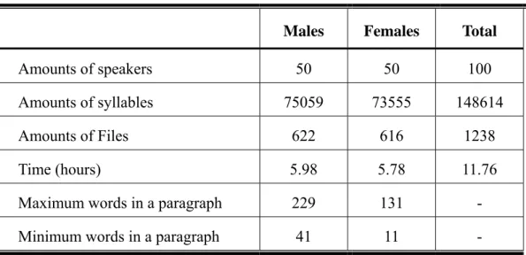
(59) Chapter 4 Experimental Results Several speaker-independent recognition experiments are shown in this chapter. The effect and performance of different front-end techniques are discussed in the experimental results. The corpus will be described in section 4.1. The experiments are divided into two parts, including the monophone-based HMM and the syllable-based HMM. The experimental results will be shown in section 4.2, and 4.3, respectively.. 4.1 Corpus The corpora employed in this thesis are TCC-300 provided by the Associations of Computational Linguistics and Chinese Language Processing (ACLCLP) and the connected-digits database provided by the Speech Processing Lab of the Department Communication Engineering, NCTU. These corpora are introduced as below. 4.1.1 TCC-300. In the speaker-independent speech recognition experiments, the TCC-300 database from the Associations of Computational Linguistics and Chinese Language Processing (ACLCLP) was used for monophone-based HMM training. TCC-300 is a collection of microphone speech databases produced by National Taiwan University (NTU), National Chiao Tung University (NCTU) and National Cheng Kung University (NCKU). In this thesis, the training corpus uses the speech databases produced by National Chiao Tung University. The speech signal is recording under the following conditions, listed in Table 4-1. The speech is saved in the MAT file format, which is a format for recording the 49.

(60) speech waveform in PCM format and, in addition, recording the condition of the environment and the speaker in detail by adding extra 4096 bytes file header into the PCM.. Table 4-1 The recording environment of the TCC-300 corpus produced by NCTU. File Format. MAT. Microphone. Computer headsets VR-2560 made by Taiwan Knowles. Sound card. Sound Blaster 16. Sampling rate. 16 kHz. Sampling format. 16 bits. Speaking style. read. The database provided by NCTU is comprised of paragraphs spoken by 100 speakers (50 males and 50 females). Each speaker read 10-12 paragraphs. The articles are selected from the balanced corpus of the Academia Sinica and each article contains several hundreds of words. These articles are then divided into several paragraphs and each paragraph includes no more than 231 words. Table 4-2 shows the statistics of the databases. Table 4-2 The statistics of the database TCC-300 (NCTU). Males. Females. Total. Amounts of speakers. 50. 50. 100. Amounts of syllables. 75059. 73555. 148614. Amounts of Files. 622. 616. 1238. Time (hours). 5.98. 5.78. 11.76. Maximum words in a paragraph. 229. 131. -. Minimum words in a paragraph. 41. 11. -. 50.