自我組織特徵映射網路於最佳化問題及其應用

國

立

交

通

大

學

電機與控制工程學系

博 士 論 文

自我組織特徵映射網路於最佳化問題及其應用

An SOM-Based Algorithm for Optimization

and Its Applications

研 究 生：陳一元

指導教授：楊谷洋 教授

自我組織特徵映射網路於最佳化問題及其應用

An SOM-Based Algorithm for Optimization

and Its Applications

研 究 生：陳一元 Student：Yi-Yuan Chen

指導教授：楊谷洋 Advisor：Kuu-Young Young

國 立 交 通 大 學

電 機 與 控 制 工 程 學 系

博 士 論 文

A Dissertation

Submitted to Department of Electrical and Control Engineering College of Electrical and Computer Engineering

National Chiao Tung University in partial Fulfillment of the Requirements

for the Degree of Doctor of Philosophy

in

Electrical and Control Engineering

July 2008

Hsinchu, Taiwan, Republic of China

自我組織特徵映射網路於最佳化問題及其應用

An SOM-Based Algorithm for Optimization

and Its Applications

研 究 生：陳一元 指導教授：楊谷洋 博士

國立交通大學電機與控制工程學系

摘要

自我組織特徵映射神經網路（SOM）已經廣泛地應用在靜態資料處理與動態資料的 分析，但利用 SOM 解決最佳化的問題的研究非常少。目前以 SOM 為基礎的最佳化演算法 對動態系統最佳化的效能還有待改進，所以在本論文中提出一自我組織特徵映射神經網 路最佳化演算法（SOMS）應用於靜態與動態最佳化問題。為了更進一步擴展它的收尋能 力，也提出一個新的鍵結值的調整規則以達到動態調整 SOM 的鄰域函數。在論文中我們 也利用 SOMS 演算法發展ㄧ智慧型雷達預估器，可在很短的時間週期內對於只有很少的 資料被雷達接收的情形下，估測目標物的運動軌跡。除此之外，當最佳化問題存在多個 最佳解時，利用一個新的 Niching 方法（即決策型競爭機制），我們也提出一個 Niching 型自我組織特徵映射神經網路最佳化演算法（NSOMS）。為了提高學習的效能且同時可以 讓最佳解的分佈結構顯現在二維的輸出空間，我們提出一新的神經元鍵結值與座標位置 的調整規則，由於新的調整規則的設計簡單而且只用到兩個學習參數分別於神經元鍵結 值與座標位置上，所以提出的 NSOMS 可以很容易地應用在不同的最佳化問題上。我們以 模擬的方式來驗證此方法的可行性，並與傳統的卡曼濾波器 (KF)，基因演算法（GA）， 與其他 SOM 最佳化演算法進行比較。

An SOM-Based Algorithm for Optimization

and Its Applications

Student： Yi-Yuan Chen

Advisor： Dr. Kuu-Young Young

Department of Electrical and Control Engineering

National Chiao Tung University

Abstract

The self-organizing map (SOM), as a kind of unsupervised neural network, has been used for both static data management and dynamic data analysis. To further exploit its search abilities, in this dissertation we propose an SOM-based search algorithm (SOMS) for optimization problems involving both static and dynamic functions. Furthermore, a new SOM weight updating rule is proposed to enhance the learning efficiency; this may dynamically adjust the neighborhood function for the SOM in learning system parameters. Based on the SOMS, we develop an intelligent radar predictor to achieve accurate trajectory estimation under the strict time constraint due to only few data are available in every short time period. Moreover, when an optimization problem has many different optimal solutions, a new niche method (deterministic competition mechanism) to extend SOM-based search algorithm (NSOMS) has been proposed for identification of multiple optimal solutions. The proposed NSOMS network structure is able to find multiple different optimal solutions and visualize distribution and structure of optimal solutions, allowing us to easily classify the optimal solutions into clusters. As a demonstration, the proposed NSOMS is applied for function optimization in a multimodal domain and also dynamic trajectory prediction involving multiple targets, with its performance compared with the genetic algorithm (GA) and other SOM-based optimization algorithms.

Acknowledgements

以最誠摯的心感謝我的指導教授楊谷洋博士，在我攻讀碩士及博士學位期間，在學 術研究領域上給予我最專業的指導與諄諄教誨，使我的博士論文得以順利完成。此外我 也從楊谷洋博士身上學習到對於研究應有的態度，懷抱著熱忱，加以認真、踏實、努力 的精神、持續不輟的耐心，才能在學術研究這條路上堅持理想，朝著目標邁進。也感謝 蘇木春教授、林進燈教授、周志成教授、林昇甫教授、陶金旭教授，以及黃士殷教授， 撥冗參與我的論文口試，你們的不吝指導與寶貴的建議，使我獲益良多，並不斷砥礪自 己精益求精。 感謝人與機器實驗室的學弟們，在論文研究上給予最佳的建議與討論，使我的研究 可以更加事半功倍。感謝我的父母、弟弟、太太、兒女，在我求學的路途上給予我最堅 定的支持與鼓勵，使我能堅持目標繼續奮鬥，因為你們的關懷與愛護，所以我能心無旁 騖的完成學業，也讓我感受到家人的關懷是支持我在求學路上最堅強、最溫暖的力量。 求學生涯告一段落，但這不代表學習的結束，而是另一階段的開始。感謝所有愛護 我的人對我的支持與鼓舞，我將帶著你們給我的信心，在學術研究的路上繼續努力！ 謹以此論文獻給愛我的師長、家人、朋友們！謝謝大家。

Contents

Chinese Abstract i

English Abstract ii

Acknowledgements iii

Contents iv

List of Tables vi

List of Figures vii

1 Introduction 1

2 Intelligent Radar Predictor 5

2.1 Dynamic Trajectory Prediction Based on Self-Organizing Map

………9

2.2 SOM Implementation

………12

2.3 Simulation

………18

3 SOM-Based Algorithm for Optimization 28

3.1 Proposed SOM-Based Search Algorithm (SOMS)

………29

3.2 Proposed Weight Updating Rule

………31

3.3 Applications

………37

3.3.1 Function Optimization

………….………38

4 Niching SOM-Based Search Algorithm (NSOMS) 52

4.1 Niching Method

………53

4.2 Proposed Niching SOMS Weight Updating Rule

……….57

4.3 Visualization of Distribution of Optimal Solutions

………62

4.4 Applications

………64

4.4.1 Function Optimization of a Multimodal Domain

………64

4.4.2 Multiple Dynamic Trajectories Prediction

………72

5 Conclusion 91

5.1 Future Research

………92

Bibliography 93

List of Tables

4.1 Comparison results for NSOMS and RCS-PSM on the 4 test functions

……….69

4.2 Comparison results for NSOMS, SOMSO-1, and SOMSO-2 on the dynamic

trajectory prediction

………..87

List of Figures

2.1 A conceptual diagram of an air-defense radar system.

..………7

2.2 System organization of the proposed intelligent radar predictor.

………11

2.3 The structure and operation in the SOM.

..………..11

2.4 The movement of the weight vector in the two-dimensional space: (a) w_j* ≠wˆ_j*

and (b) wj* =wˆj*.

………..………13

2.5 Simulation results for trajectory prediction using the SOM and the Kalman filter

with good estimates of both the initial condition and noise distribution: (a) the ideal

and measured TBM trajectories, (b) the estimated position error by using the SOM

and Kalman filter, and (c) the movement of the weight vector w_j during the SOM

learning process.

………..21

2.6 Simulation results for trajectory prediction using the SOM and the Kalman filter

with a good estimate of the initial condition but bad estimate of the noise

distribution: (a) the ideal and measured TBM trajectories, (b) the estimated position

error by using the SOM and Kalman filter, and (c) the movement of the weight

vector w_j during the SOM learning process.

………..23

2.7 Simulation results for trajectory prediction using the SOM and the Kalman filter

with a bad estimate of the initial condition but good estimate of the noise

distribution: (a) the ideal and measured TBM trajectories, (b) the estimated position

error by using the SOM and Kalman filter, and (c) the movement of the weight

vector wj during the SOM learning process.

……….………….24

2.8 Simulation results for trajectory prediction using the SOM and the Kalman filter

ideal and measured TBM trajectories, (b) the estimated position error by using the

SOM and Kalman filter, and (c) the movement of the weight vector w_j during the

SOM learning process.

……….……25

2.9 Results by applying the SOM to predict the actual TBM trajectory.

………..26

3.1 Conceptual diagram of the organized search in a 2-D SOM: the solution is (a)

within the estimated range and (b) outside of the estimated range.

………...30

3.2 Proposed SOM-based algorithm for optimization.

………..33

3.3 Structure and operation of the SOM in the SOMS.

………..33

3.4 Center and width adjustment for the neighborhood function G w( j i_,( ))k , when (a)

(

*

)

2 2 ,( ) ei _{j i} i w −w k ≥

σ

, and (b).

(

*

)

2 2 ,( ) ei j i i w −w k <σ .

……….36

3.5 Minimization of the 2-D Griewant function using the SOMS and GA with the

optimal solution outside of the estimated region: (a) minimal function values

*

( j ( ))

O w k during the learning process, (b) weight vector movement in the SOM, and (c) weight vector movement in the GA.

………41

3.6 Minimal function values O(w_j*( ))k during the learning process for the mini-

mization of the 30-D Rosenbrock function using the SOMS, GA, and SOMO.

…….42

3.7 Simulation results for dynamic trajectory prediction using the SOMS, SOMSO, and

GA with a good estimate of the initial state: (a) the estimated position error in the

X-direction and (b) the variation of the neighborhood function F(w_j( ))k during the SOMS learning process.

………..50

3.8 Simulation results for dynamic trajectory prediction using the SOMS, SOMSO, and

GA with a bad estimate of the initial state.

………51

4.1 Optimization during learning process: (a) without the niching method, (b) with the

4.2 Proposed Niching SOM-based search algorithm.

………56

4.3 Structure and operation of the SOM in the NSOMS.

………56

4.4 Three multimodal functions. (a) F1: uniform sine function, (b) F2: nonuniform sine

function, and (c) F3: Shekel’s Foxholes function.

………..67

4.5 Convergence comparisons for F3 function: (a) the variation of the number of

maintained peaks and (b) the variation of the maximum peak ratio during the

NSOMS learning process.

………..70

4.6 The results obtained by the NSOMS for F4 function: (a) projection result in the 2D

neuron space, and (b) final neighborhood function values.

……….71

4.7 Simulation results for the multiple trajectories prediction using the NSOM,

SOMSO-1, and SOMSO-2 with a good estimate of the initial state: (a) the ideal

and measured TBM trajectories, (b)-(d) the estimated initial state error by using the

NSOM, SOMSO-1, and SOMSO-2.

……….77

4.8 Final results obtained by the NSOMS for the multiple trajectories prediction: (a)

projection result in 2D neuron space and (b) finial neighborhood function values.

…78

4.9 Simulation results for multiple trajectories prediction using the NSOM, SOMSO-1,

and SOMSO-2 with a bad estimate of the initial state: (a) the ideal and measured

TBM trajectories, (b)-(d) the estimated initial state error by using the NSOM,

SOMSO-1, and SOMSO-2.

………81

4.10 Final results obtained by the NSOMS for the multiple trajectories prediction : (a)

projection result in 2D neuron space and (b) finial neighborhood function values.

...82

4.11 Performance for different network sizes using the NSOMS, SOMSO-1, and

SOMSO-2.

……….84

4.12 Performance for different parameters using the NSOMS, SOMSO-1, and

SOMSO-2.

……….86

and SOMSO-2…

………89

4.14 Performance of 5 runs with the different initial weights using the NSOMS,

Chapter 1

Introduction

The self-organizing map (SOM), as a kind of unsupervised neural network, is performed in a self-organized manner in that no external teacher or critic is required to guide synaptic changes in the network [4, 22]. By contrast, for the other two basic learning paradigms in neural networks, supervised learning is performed under the supervision of an external teacher [14] and reinforcement learning involves the use of a critic that evolves through a trial-and-error process [3]; these other two also demand the input-output pairs as the training data. The appealing features of learning without needing the input-output pairs makes the SOM very attractive when dealing with varying and uncertain data. In its many applications, the SOM has been used for both static data management and dynamic data analysis, such as data mining, knowledge discover, clustering, visualization, text archiving, image retrieval, speaker recognition, mobile communication, robot control, identification and control of dynamic systems, local dynamic modeling, nonlinear control, and tracking moving objects [1, 2, 14, 22, 24, 31, 36, 37, 38, 42]. There have also been many approaches proposed to improve or modify the original SOM algorithm for different purposes [2, 13, 19, 37, 43, 45, 47]. However, from our survey, its search abilities have not been adequately

exploited yet [7, 12, 16, 29, 30, 40]. This need thus motivates us to propose an SOM-based search algorithm (SOMS) for both static and dynamic functions.

In recent years, some new research studies have turned to tackle the continuous opti-mization problems based on the self-organizing map. Michele et al. proposed an optimiza-tion method based on the Kohonen SOM evoluoptimiza-tion strategy (KSOM-ES) [29]. Su et al. proposed the SOM-based optimization algorithm (SOMO) [40]. An self-organizing and self-evolving agents (SOSENs) neural network that combines multiple simulated anneal-ing algorithms (SAs) and SOM algorithm have also been proposed [44]. Our proposed SOMS will extend the application further to optimization problems involving dynamic functions. When searching for a dynamic function, the goal may be to look for a set of optimal parameters that lead to the desired performance of the dynamic system from limited measured data. In this dissertation we first apply the self-organizing map (SOM) to develop an intelligent radar predictor. With the few radar data read into the predictor in each time interval and a simplified dynamic model of the moving target, the SOM learns to estimate the initial state of the target trajectory in each learning cycle, and will gradually converge to the optimal initial state. To achieve high learning efficiency under such widely varying parameters, we propose a new weight updating rule which may dynamically adjust the shape and location of the neighborhood function for the SOM, in an individual basis, in learning the system parameters. Thus, the proposed SOMS should be able to execute both system performance evaluation and the subsequent search in a real-time manner.

Many optimization problems often have more than one optimal solutions in the feasible domain [15, 34, 41]. If more different optimal solutions can be found, it is advantageous for us to have the right of choice. Although many global optimization techniques based

on population evolutionary have been successfully applied to find the global optimum [12, 17, 21], they cannot be directly applied to search for multiple solutions through one search process in a multimodal domain. Mahfoud proposed the niching methods to iden-tify multiple optima in a multimodal domain [28]. When many optimal solutions are obtained, how to classify the set of optimal solutions and select one useful solution is difficult, and in particular depends on the number of the optimal solutions and the size of dimension. Igarashi used GA to find many different optimal solutions repeatedly and applied the SOM for visualization and clustering of optimal solutions in 2-D output spaces [15]. The visualization of high-dimensional data is one of the well-known merits of the SOM. However, the SOM algorithm proposed in [15] was not applied to optimization. Although the SOM has been used to tackle the optimization problems [29, 40, 44] and its performances have been manifested better than other search algorithms such as SA [21], PSO [17], DE [25], and GA [12], their search abilities were still not well exploited in finding multiple optimal solutions. Meanwhile, it did not simultaneously provide vi-sualization of the distribution of optimal solutions, either. Thus, we further propose a niching SOM-based search algorithm (NSOMS) for identification and visualization of the multiple optimal solutions.

This new niching method is proposed to extend the SOMS by defining subpopulations (subspaces) in a multimodal domain. With the proposed niching weight-updating rule, the niche location located on the winning weight site will be moved to approach the real peak location of a multimodal domain gradually. Thus, with many different niches set, the NSOMS can be applied to searching for multiple optimal solutions. For visualization of distribution of optimal solutions, the concept of the double SOM (DSOM) [39], which updates the weight vectors together with the two-dimensional position vector of the neu-ron, is employed in the proposed NSOMS. The optimal solutions in the parameter space

are mapped onto a two-dimensional (2-D) neuron space. Through this map it allows us to classify the optimal solutions into clusters. We then apply proposed NSOMS to function optimization in a multimodal domain and multitarget tracking problem simultaneously with data sent from multiple sensors. The rest of this dissertation is organized as follows. The proposed intelligent radar predictor including SOM and the performance of the SOM compared with that of the Kalman filtering are discussed in Chapter 2. The proposed SOMS with dynamic weight updating rules and also the performance of the SOM com-pared with that of the SOMO and GA are presented in Chapter 3. The proposed NSOMS with the new weight updating rules for multiple optimal solutions and visualization of dis-tribution of optimal solutions are described in Chapter 4. Finally, conclusions and some future works are given in Chapter 5.

Chapter 2

Intelligent Radar Predictor

Nowadays, the tactical ballistic missiles (TBM) can be as fast as 3-7 Mach. For successful tracking of the TBM moving in so high a speed, the air-defense radar system should be capable of trajectory prediction to catch up with the movement of the TBM. It is then imperative to develop a radar predictor that can estimate the TBM trajectory using the radar data. Due to the strict time constraint, only very few radar data are available for each prediction during the tracking. In addition, the prediction needs to be executed in real time. Under such circumstances, the radar predictor should possess certain degree of intelligence to cope with the limited and possibly noisy radar data. The challenge of developing an intelligent radar predictor for accurate trajectory estimation motivates the study in this dissertation.

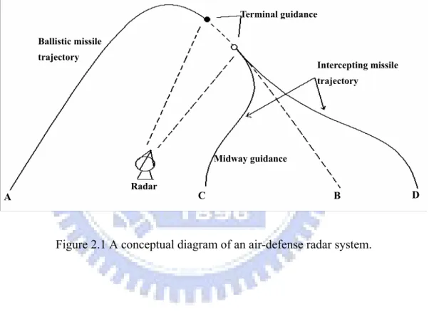
Before discussing the proposed intelligent radar predictor, we first briefly describe an air-defense radar system, as shown in Figure 2.1 [23]. In Figure 2.1, a TBM is launched from location A; the radar system then tracks its trajectory, in addition to predicting the possible landing site, location B. Under successful tracking, the radar system can then

guide the intercepting missile to penetrate into the predicted trajectory of the incoming TBM, and destroy it as early as possible. From the different launching site relative to location B, location C or D, the intercepting missile may take different route to enter the predicted TBM trajectory, as shown in Figure 2.1. To let the intercepting missile follow the trajectory shown in Figure 2.1, missile guidance law is demanded. By commanding the acceleration of the missile proportional to the angular rate of some desired direction, the guidance law will turn the heading of the missile toward that direction as rapidly as possible [23, 46]. As the intruding missile is in such a high speed and small volume, the design of guidance law for the intercepting missile is very challenging.

Missile guidance can basically be divided into two stages: midway guidance and termi-nal guidance. During the midway guidance stage, the information from the ground radar is used to guide the intercepting missile. When the target trajectory can be precisely predicted, the intercepting missile may not need to chase after an extremely fast target, but just move toward the predicted target location. After the intercepting missile is led close to the target, the seeker, as an active radar equipped on the missile, may then take over and proceed with the terminal guidance. As the intruding TBM may be capable of escaping, delicate guidance laws need to be installed in the seeker to provide more complex maneuvering. It can be seen that control load for missile interception in both stages of guidance can be tremendously alleviated, if the radar system is able to estimate the TBM trajectory accurately. Meanwhile, trajectory prediction can also provide the possible TBM landing location, and thus be helpful in determining a proper location and direction to launch the intercepting missile.

One famous approach for trajectory prediction is the Kalman filtering, which has been widely used in predicting the movements of the satellites, airplanes, ships, etc. [32].

Figure 2.1 A conceptual diagram of an air-defense radar system. ! Ballistic missile trajectory Intercepting missile trajectory Terminal guidance Radar M idway guidance C A B D

By knowing the dynamic model of the moving target, the Kalman filter in general yields satisfactory performance when the statistics of the environmental noises and good guesses of the initial conditions can be obtained in advance. However, the Kalman filtering may not be suitable for unknown, noisy environments. To tackle the situation aforementioned, researches have been dedicated to build mathematical models, perform statistical data analysis, and make the Kalman filter more adaptive [5, 9, 27]. It is by no means an easy task to cope with the complexity involved in modeling, though. As an alternative, the learning mechanism has been used to assist the Kalman filter, since it is model-free and computational efficient after training. Among them, Roberts et al. proposed a neurofuzzy estimator to improve the Kalman filter initialization [33]. Chin proposed incorporating the neural network into the Kalman filter configuration to deal with the multi-target tracking problem [6].

The SOM, first introduced by Kohonen, transforms input vectors into a discrete map (e.g., a 2-D grid of neurons) in a topological ordered fashion adaptively [22, 37]. During each iteration of learning, the each neuron competes with each other to gain the oppor-tunity to update its weight, and the vector that generates the output most close to the desired value (vector) is chosen as a winner. Because the SOM allows local interaction between neighboring neurons, the weights of the winner and also its neighbors are all updated. Through repeated weight modification, a cluster (or clusters) may form and become more and more compact until a final configuration develops. The SOM thus has a structure very suitable for parallel processing. We further exploit this parallelism and design an organized search accordingly. In other words, we take advantage of the SOM in its distribution of the neurons in a grid pattern and the presence of local interaction in between the grid.

The SOM in the proposed predictor is in fact used as a search mechanism, and the simplified TBM dynamic model as a reference for the SOM to approach the neighborhood of the TBM. The employment of the SOM in this way is different from those in most of its previous applications, and well exploits it capability in searching. The proposed intelligent radar predictor including SOM is described in next section.

2.1

Dynamic Trajectory Prediction Based on

Self-Organizing Map

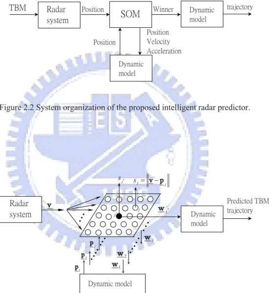
Figure 2.2 shows the system organization of the proposed intelligent radar predictor. For an incoming TBM, the predictor uses the measured position data sent from the radar to predict the TBM trajectory. The main module in this predictor is the SOM [22]. We may distribute the possible positions and velocities of the missile (as weight vectors) into the network in an organized fashion. Under this arrangement, the searches among the neurons are closely related through the grid, leading to a more rapid convergence. On the other hand, when the estimation is inaccurate, the search, still organized, may take longer time to converge to the optimal solution.

The adoption of the SOM to realize this intelligent radar predictor is that it does not demand input-output pairs for on-line prediction when facing unknown environments. Thus, the genetic algorithm (GA) may also be a possible alternative [12]. Genetic al-gorithms are search alal-gorithms based on the mechanics of natural selection and natural genetics. It employs multiple concurrent search points called chromosomes and evaluates the fitness of each chromosome. The search procedure uses random choice as a tool to guide a highly exploitative search through a coding of a parameter space. We consider

the SOM is more suitable than the GA for this trajectory tracking problem. The rea-son is that the connection among the possible initial states for missile launching is not utterly random. The SOM better exploits the relationship between the initial state and its resultant TBM trajectory, leading to a somewhat guided search. In addition, the GA is in general more time-consuming. As the prediction needs to be accomplished within a limited amount of time, the efficiency of the network is crucial.

In this TBM tracking application, the SOM is used to estimate the initial position, velocity, and acceleration of the TBM using the measured position data from the radar. Thus, if the dynamic model of the TBM is available, the entire TBM trajectory can be derived using those estimated initial position, velocity, and acceleration as the initial state for the dynamic model. Through a learning process, the SOM determines a most probable initial state by comparing the measured position data with the predicted TBM position trajectories derived from a number of possible initial states selected from a predicted range. The process of how the SOM learns to estimate the initial state is as follows. First, a number of vectors, each of which contains a possible initial state, are selected and stored into the neurons of the SOM. During each time interval, the SOM sends these vectors to the dynamic model of the TBM to compute the corresponding trajectories. By comparing the predicted trajectories with the measured radar data, the vector corresponding to the most accurate predicted trajectory is chosen as the winner. The weights of this winner and its neighbors are updated, and the network will eventually converge to the optimal initial state. To note that, even the optimal initial state is not within those vectors initially selected from the predicted range, the SOM is able to move these vectors out of their original locations and guide them to converge to the optimal initial state. Implementation details of the SOM for trajectory prediction are given in next section.

ʳ

ʳ

Figure 2.2 System organization of the proposed intelligent radar predictor.

Figure 2.3 The structure and operation in the SOM.

! ˥˴˷˴̅ʳ ̆̌̆̇˸̀ʳ ʳ

˦ˢˠʳ

˗̌́˴̀˼˶ʳʳ ̀̂˷˸˿ʳ ˧˕ˠʳ ˣ̂̆˼̇˼̂́ʳ ˩˸˿̂˶˼̇̌ʳ ˔˶˶˸˿˸̅˴̇˼̂́ʳ ˣ̂̆˼̇˼̂́ʳ ˣ̅˸˷˼˶̇˸˷ʳ˧˕ˠʳ ̇̅˴˽˸˶̇̂̅̌ʳ ˣ̂̆˼̇˼̂́ʳ ʳ ˗̌́˴̀˼˶ʳ ̀̂˷˸˿ ˪˼́́˸̅ʳ * j s ˗̌́˴̀˼˶ʳʳ ̀̂˷˸˿ʳ ˣ̅˸˷˼˶̇˸˷ʳ˧˕ˠʳ ̇̅˴˽˸˶̇̂̅̌ʳ ˗̌́˴̀˼˶ʳ̀̂˷˸˿ ˥˴˷˴̅ʳ ̆̌̆̇˸̀ʳ j p 2 p 1 p * j w j _j s v!p j j* v j w 2 w 1 w

2.2

SOM Implementation

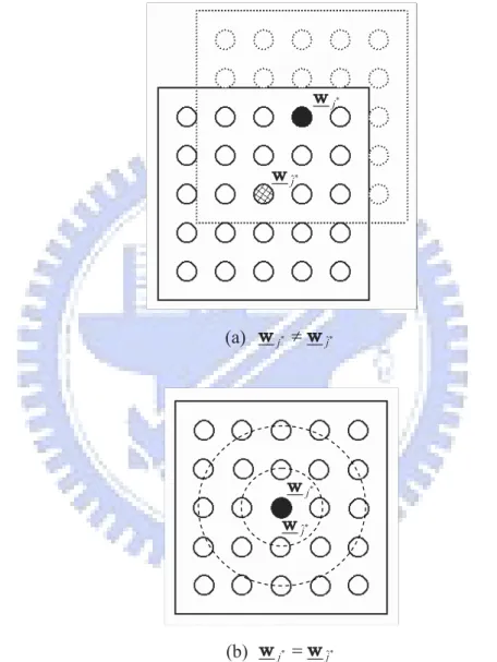
For this TBM tracking application, the SOM needs to tackle the spatio-temporal data, instead of the spatial data it usually deals with. Therefore, a dynamic model that describes the behavior of the TBM is included in the intelligent radar predictor. By combining the SOM with the dynamic model, the SOM is able to tackle the spatio-temporal radar data. Figure 2.3 shows the structure and operation in the SOM. A 2D SOM is used for illustration in Figure 2.3, and the SOM can also be three-dimensional or other according to the applications. Each time a certain number of new measured position data v are sent in from the radar system, the SOM is triggered to operate. And, it will gradually converge to an optimal prediction along with the increase of the measurement data and learning time. In Figure 2.3, for each neuron j in the SOM, it contains a vector of a possible initial state w_j and generates an output sj. By sending wj to the dynamic model, sj is

computed as the difference between v and the predicted trajectory p_j. Of all the neurons, the neuron j∗ _{with the smallest output s}

j∗ is chosen as the winner. When the weight of

this winning neuron j∗ _{differs from that of the previous winner ˆj}∗ _{(i.e., w}

j∗ 6= w_ˆj∗), the

weights of ˆj∗ _{and its neighbors will be updated in a manner that moves these weight}

vectors toward neuron j∗_{, as shown in Figure 2.4(a). When j}∗ _{is the same as ˆj}∗ _(i.e.,

w_j∗ = w_ˆj∗), the weights will then be updated so as to let the weight vectors form more

and more compact clusters centering at neuron j∗_{, as shown in Figure 2.4(b). Under}

successful learning, the SOM will finally converge to a predicted optimal initial state. Several parameters need to be determined in implementing this SOM, including the learning rate, topological neighborhood function, and number of radar data used for sj

computation. The selection of the learning rate η depends on the closeness of wj∗(k) and

!

(a) w_j* wˆ_j*

(b) w_j* w_ˆj*

Figure 2.4 The movement of the weight vector in the two-dimensional

space: (a) w_j* w and (b)ˆ_j* !w_j* w .ˆ_j*

* j w * ˆj w * j w * ˆj w

process and choose η(k) in the kth stage of learning to be close to 1. And when they almost coincide, we slow down the learning gradually and determine η(k) according to Eq.(2.1): η(k) =    η0(1 − k/τ ), f or k ≤ τ0 < τ η1(1 − τ0/τ ), f or k > τ0 (2.1)

where η0 and η1 are constants smaller than 1, and τ and τ0 time constants. Other types

of functions can also be used, for instance,

η(k) = η1· e−k/τ + η0 (2.2)

Because the weight updating also includes the neighbors of the winning neuron, the topo-logical neighborhood function hj∗ needs to be chosen. We adopt the Gaussian

neighbor-hood function for hj∗(k) [17]:

hj∗(k) = exp(−

d2

j,j∗

2σ2) (2.3)

where dj,j∗ is a lateral connection distance between neural j and j∗, and σ the width. For

the sake of efficiency in computing sj, not all the accumulated measured radar data will be

used to compare with the predicted trajectory. Under such selection of the learning rate and neighborhood function, they will force the minimization of the difference between the weight of the winning neuron and those corresponding to every neuron within its neighborhood in each learning cycle. The learning in the algorithm will thus converge eventually.

Based on the discussions above, we developed the SOM learning algorithm. Before the description of the algorithm, we first introduce a simplified dynamic model of the TBM. With the model, the SOM can obtain p_j by sending wj into it. This dynamic model is

formulated as

x(k + 1) = A(k)x(k) + Γ(k)ξ(k) (2.4) v(k) = C(k)x(k) + µ(k) (2.5)

where

x(k) : n-dimensional state vector at the kth stage A(k) : n × n transition matrix

Γ(k) : n × r input distribution matrix

ξ(k) : r-dimensional random input vector

v(k) : m-dimensional output vector

C(k) :m × n observation matrix

µ(k) : m-dimensional random disturbance vector

with ξ(k) and µ(k) assumed to be white Gaussian with the following properties:

E[ξ(k)] = 0 (2.6)

E[ξ(j)ξ(k)t_{] = Qδ}

E[µ(k)] = 0 (2.8)

E[µ(j)µ(k)t_{] = Rδ}

jk (2.9)

E[ξ(j)µ(k)t_{] = 0 (2.10)}

where E[·] stands for the expectation function, Q and R the covariance matrix of the input noise and output noise, respectively, and δjk the Kronecker delta function. In using

the dynamic model, the SOM is not necessarily aware of its statistical properties. By contrast, the Kalman filter needs to know the noise distribution in the dynamic model and also a guess on the system’s initial state for trajectory prediction. As the covariance matrices Q and R may be uncertain and varying in noisy, unknown environments, their estimated values are possibly imprecise, even incorrect. Thus, the Kalman filter may not be that effective under such circumstances. The reason that the SOM is more robust to the uncertainty of the dynamic model than the Kalman filter and why it does not require a guess on the initial state may be because it contains a large number of self-organizing neurons in the network. Via learning, these neurons provide many different directions to search for the optimal initial state.

In responding to the three variables, the launching position, velocity, and acceleration of the TBM, a 3D SOM is used for trajectory prediction. The SOM learning algorithm is organized as follows:

SOM Learning Algorithm: Predict an optimal initial state for an incoming TBM in a real-time manner using the measured position radar data.

Step 1: Set the stage of learning k = 0. Estimate the ranges of the possible initial position, velocity, and acceleration of the TBM, and randomly store the possible initial states wj(0) into the neurons, where j = 1, . . . , N3, N ×N ×N the total number of neurons

in the 3D space. Select neuron ˆj∗ _{in the center of the neuron space as the winning neuron.}

Step 2: Send w_j(k) into the dynamic model, described in Eqs.(2.4)-(2.5), to compute p_j(k).

Step 3: For each neuron j, compute its output sj as the difference between the measured

position data v(k) and p_j(k):

sj(k) = k X i=0 ° ° °p_j(i) − v(i) ° ° ° (2.11)

Find the winning neuron j∗ _{with the minimum s} j∗(k): sj∗(k) = k X i=0 ° ° °p_j∗(i) − v(i) ° ° °= min j k X i=0 ° ° °p_j(i) − v(i)°°° (2.12)

Step 4: Update the weights of the previous winning neuron ˆj∗ _{and its neighbors within}

h_ˆj∗(k) using the following two rules:

If j∗ _{6= ˆj}∗_{, then w}

j(k + 1) = wj(k) + η(k)hˆj∗(k)(w_j∗(k) − w_ˆj∗(k)) (2.13)

If j∗ = ˆj∗, then w_j(k + 1) = w_j(k) + η(k)h_ˆj∗(k)(w_j∗(k) − w_j(k)) (2.14)

where η(k) is the learning rate described in Eq.(2.1) and h_ˆj∗(k) the neighborhood function

in Eq.(2.3).

Step 5: Check whether the difference between w_j∗(k) of the winning neuron j∗and w_j(k)

corresponding to every neuron j within hj∗(k) is smaller than a prespecified value ²:

max

If Eq.(2.15) does not hold, let k = k + 1, and when k is smaller than a prespecified maximum value, go to Step 2; otherwise, the prediction process is completed and output the optimal initial state to the dynamic model to derive the TBM trajectory. Note that the value of ² is empirical according to the demanded resolution in learning, and we chose it very close to zero.

2.3

Simulation

To demonstrate the effectiveness of the proposed intelligent radar predictor, we performed a series of simulations based on using both the generated and real radar data. The results were compared with those using the Kalman filtering. Via coordinate transformation, the trajectory of the incoming TBM was described in a 2D (X ×Y ) space. Because simulation results were similar for the motions in the X and Y directions, we only discussed the motion in the X direction to simplify the illustration. Thus, according to Eq.(2.4), the dynamic model for the TBM is formulated as

x(k + 1) = A(k)x(k) + ξ(k) (2.16) with x(k) =      x(k) ˙x(k) ¨ x(k)     , A(k) =      1 T T2_/2 0 1 T 0 0 1     , ξ(k) =      0 0 ξ(k)      (2.17)

in the X direction, respectively, T the sampling time, and ξ(k) the noise and modeling error that perturbs the target acceleration, with a zero mean and constant variance σ2

a.

And, according to Eq.(2.5), the measured radar position v(k) is formulated as

v(k) = x(k) + µ(k) (2.18) where µ(k) is the measurement noise with a zero mean and constant variance σ2

m. The

ranges of the possible initial states w_j(0) were predicted to be

−1000 m ≤ x(0) ≤ 1000 m

−2000 m/s ≤ ˙x(0) ≤ 2000 m/s(5.88Mach) −50 m/s2 _{≤ ¨x(0) ≤ 50 m/s}2_.

(2.19)

Within the ranges described in Eq.(2.19), the possible launching position, velocity, and acceleration of the TBM were selected and stored into the 125 neurons of the 3D SOM. The variances, σ2

a and σ2m, described in Eqs.(2.17)-(2.18), are chosen to be (0.32m/s2)2

and (200m)2_{, respectively. The sampling time T was chosen to be 1s. The number of}

learning is set to be 20 during each stage of learning.

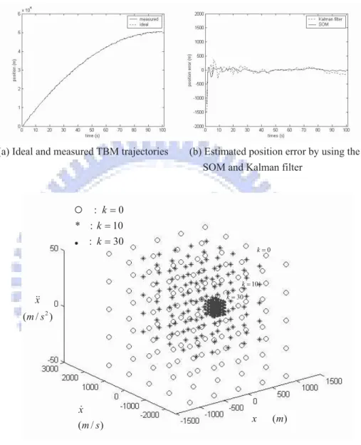
We first applied the SOM and Kalman filter for trajectory prediction under the condi-tion that good estimates of both the initial state and noise distribucondi-tion were available. The ideal initial state of the target was assumed to be (500m, 1000m/s(2.94Mach), −10m/s2_),

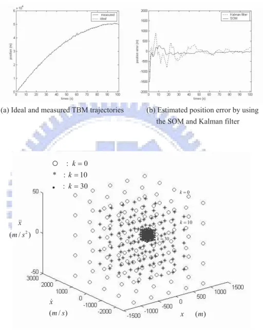
which was within the predicted ranges. And the variance of the measurement noise was set to be the same as the predicted (200m)2_{. The ideal and measured TBM trajectories were}

shown in Figure 2.5(a). Both the SOM and Kalman filter predicted the (k + 1)th state quite well, and thus resulted in very small estimated position errors, except in the initial stage of the prediction, as shown in Figure 2.5(b). Figure 2.5(c) shows the movement of the weight vector w_j during the SOM learning process. In Figure 2.5(c), the weight

vectors of the neurons in the SOM continued to move closer and closer during learning, and finally converged to a very small region, since the winning neuron was already within the predicted region from the beginning.

In the second set of simulations, we intended to investigate the performances of the SOM and Kalman filter under the following three situations: (1) good estimate of the initial state, but bad estimate of the noise distribution, (2) bad estimate of the initial state, but good estimate of the noise distribution, and (3) bad estimates of both the initial state and noise distribution. For Case 1, the ideal initial state of the target was still set to be (500m, 1000m/s(2.94Mach), −10m/s2_{), but the variance of the measurement noise was}

enlarged to be (400m)2_{. The ideal and measured TBM trajectories were shown in Figure}

2.6(a). With a bad estimate of the noise distribution, the performance of the Kalman filter degraded, but the SOM still performed well, as shown in Figure 2.6(b). In Figure 2.6(c), the neurons in the SOM exhibited similar behaviors as those shown in Figure 2.5(c). For Case 2, the ideal initial state was assumed to be (5000m, 3000m/s(8.82Mach), −60m/s2_),

which was outside the predicted ranges. The variance of the measurement noise was set to be (200m)2_{. The ideal and measured TBM trajectories were shown in Figure 2.7(a). With}

a bad estimate of the initial state, the performances of both the SOM and Kalman filter degraded in the initial stage of the prediction, but the SOM achieved better prediction later, as shown in Figure 2.7(b). Correspondingly, the weight vectors of the neurons in the SOM moved from the original predicted region outward to the ideal initial state, and finally converged to the desired location, as shown in Figure 2.7(c). For Case 3, the ideal initial state was assumed to be (5000m, 3000m/s(8.82Mach), −60m/s2_{), and the}

variance of the measurement noise set to be (400m)2_{. The ideal and measured TBM}

trajectories were shown in Figure 2.8(a). With bad estimates of both the initial state and noise distribution, the Kalman filter perform poorly, but the SOM still achieved

(a) Ideal and measured TBM trajectories (b) Estimated position error by using the SOM and Kalman filter

!

(c) Movement of the weight vector wj during the SOM learning process

Figure 2.5 Simulation results for trajectory prediction using the SOM and the Kalman filter with good estimates of both the initial condition and noiseʳ distribution: (a) the ideal and measured TBM trajectories, (b) the estimated position error by using the SOM and Kalman filter, and (c) the movement

of the weight vector wj during the SOM learning process.

( ) x m ( / ) x m s 2 ( / ) x m s : k 0 * : k 10 : k 30 30 k 10 k 0 k

satisfactory performance, as shown in Figure 2.8(b). In Figure 2.8(c), the neurons in the SOM exhibited similar behaviors as those shown in Figure 2.7(c).

For further investigation, we performed simulations for input noises with the compo-nents in both x and y directions and also the condition of a non-zero expectation for these two components. The results show that when the expectation values were small, the in-telligent radar predictor still worked quite well. We also performed simulations based on using the genetic algorithm. During the simulations, we first randomly selected the initial populations. When the optimal initial state did not fall within the selected ranges, the GA converged very slowly. We then modified the population size and crossover and mutation probabilities to speed up its convergence rate. However, it was not that straightforward to determine these parameters properly, and the process was time-consuming. From the simulation results, we conclude that the proposed intelligent predictor performed better than the GA for this trajectory tracking problem.

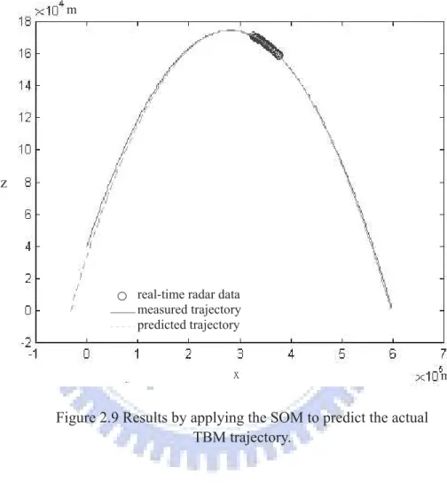
From the results shown in Figures 2.6-2.8, we found that bad estimates of the initial state and noise distribution much affected the performance of the Kalman filter. By contrast, their influence on the SOM was mostly at the initial stage of the prediction. After the transient, the SOM still managed to find the optimal initial state via learning. With its robustness to uncertainty and efficiency in computation, we then used the SOM to predict the TBM trajectory based on using real radar data. The radar data, provided by the military research center, had been modified due to the security consideration. The SOM used only a small number of radar data, marked by the ◦ sign in Figure 2.9, to predict the TBM trajectory. In Figure 2.9, the predicted trajectory well approximated the measured one, demonstrating the ability of the SOM to deal with real radar data.

(a) Ideal and measured TBM trajectories (b) Estimated position error by using the SOM and Kalman filter

!

(c) Movement of the weight vector wj during the SOM learning process!

Figure 2.6 Simulation results for trajectory prediction using the SOM and the Kalman filter with a good estimate of the initial condition but bad estimate of the noiseʳ distribution: (a) the ideal and measured TBM trajectories, (b) the estimated position error by using the SOM and Kalman

filter, and (c) the movement of the weight vector wj during the SOM

learning process. ( ) x m ( / ) x m s 2 ( / ) x m s : k 0 * : k 10 : k 30 10 k 0 k 30 k

(a) Ideal and measured TBM trajectories (b) Estimated position error by using the SOM and Kalman filter

(c) Movement of the weight vector wj during the SOM learning process

Figure 2.7 Simulation results for trajectory prediction using the SOM and the Kalman filter with a bad estimate of the initial condition but good estimate of the noiseʳ distribution: (a) the ideal and measured TBM trajectories, (b) the estimated position error by using the SOM and Kalman

filter, and (c) the movement of the weight vector wj during the SOM

learning process. ( ) x m ( / ) x m s 2 ( / ) x m s : k 0 * : k 5 + : k 10 : k 30 0 k 5 k 10 k 30 k

(a) Ideal and measured TBM trajectories (b) Estimated position error by using the SOM and Kalman filter

(c) Movement of the weight vector w_j during the SOM learning process

Figure 2.8 Simulation results for trajectory prediction using the SOM and the Kalman filter with bad estimates of both the initial condition and the noiseʳ distribution: (a) the ideal and measured TBM trajectories, (b) the estimated position error by using the SOM and Kalman filter, and (c) the

movement of the weight vector wj during the SOM learning process.

( ) x m ( / ) x m s 2 ( / ) x m s : k 0 * : k 5 + : k 10 : k 30 0 k 5 k 10 k k 30

!

Figure 2.9 Results by applying the SOM to predict the actual TBM trajectory. ʳ m ̋ʳ z m

real-time radar data measured trajectory predicted trajectory

trajectory estimation. With a simplified target dynamic model, the unsupervised SOM in the predictor can achieve salient prediction in the presence of noise, even with a bad estimate of the initial state. The performance of the SOM has been compared with mainly that of the Kalman filtering. The simplified TBM dynamic model used in the current stage of the study may account for only the coarse behavior of the TBM. Nevertheless, even with only the general information provided by this simplified model, the proposed intelligent radar predictor has been able to catch up with the TBM, as demonstrated in the simulations based on using the real radar data.

Chapter 3

SOM-Based Algorithm for

Optimization

Although the SOM has been widely used in many diverse tasks, few studies are available for applying the SOM as a search mechanism. Recently, some researchers have exploited its ability in search [7, 29, 40]. Michele et al. proposed a learning algorithm for optimiza-tion based on the Kohonen SOM evoluoptimiza-tion strategy (KSOM-ES) [29]. In this KSOM-ES algorithm, the adaptive grids are used to identify and exploit search space regions that maximize the probability of generating points closer to the optima. Su et al. proposed an SOM-based optimization algorithm (SOMO) [40]. Through the self-organizing process in SOMO, solutions to a continuous optimization problem can be simultaneously explored and exploited. The point about applying the SOM as a search mechanism is that each weight vector represents a possible solution of the objective function. Through the fitness function the winner will be determined with the largest fitness and updating the weights of the winner and its neighbors, all the weights will be moved to explore and exploit the optimization space for the searching process. A major drawback is that the SOMO and

KSOM-ES converge very slowly if the optimal solution falls outside the estimated range. Because of the influence of noise the search direction is not correct probably. Meanwhile the step size is reduced continually. Eventually the optimal solution is probably outside the search range. In the dynamic optimization the search direction and step size are hard to determine effectively in noisy and unknown environment. Thus, in this chapter a new SOM weight updating rule based on a heuristic techniques is proposed to deals properly with these problems and enhance the learning efficiency; this may dynamically adjust the neighborhood function for the SOM in learning system parameters, discussed in next Section.

3.1

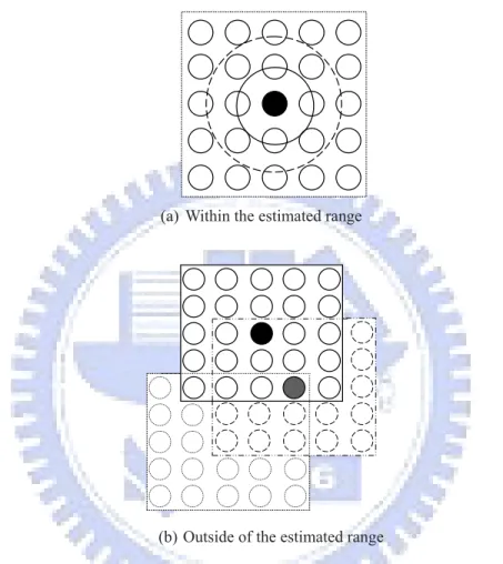
Proposed SOM-Based Search Algorithm

Figure 3.1 shows the conceptual diagram of the organized search in a 2-D SOM. Note that Figure 3.1 is slight different from Figure 2.4 in that the weight of the previous winner replaced by the average of all weights. Figure 3.1(a) shows a case where the solution is within the estimated range. In this case, the weights of the neurons are updated so as to make the weight vectors converge to a compact cluster centering at the optimal solution. Figure 3.1 (b) shows the case where the solution is outside the estimated range. The winner will be located at the corner of the SOM initially. During the next learning epoch, it is moved to the center of the SOM. The learning will continue until the solution falls within the new estimated range. The search will then follow the process shown in Figure 3.1(a) to converge to the optimal solution.

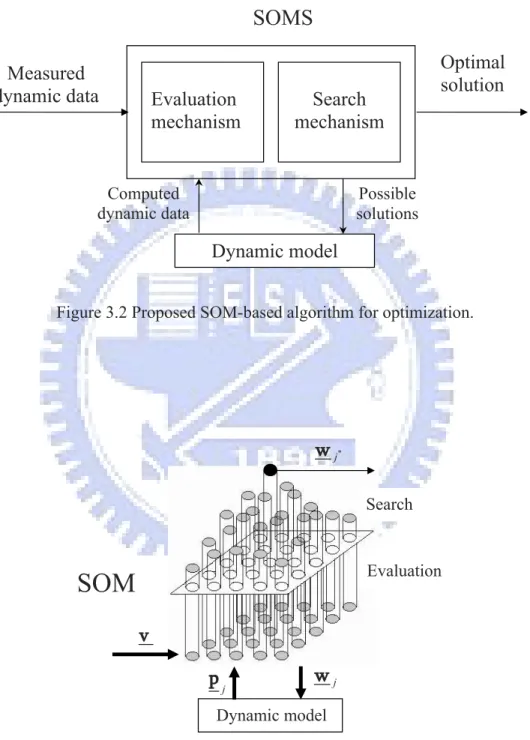
Figure 3.2 shows the proposed SOMS, which consists of mainly the evaluation and search mechanisms and the dynamic model stands for the target system. Initially, the

(a) Within the estimated range

(b) Outside of the estimated range

Figure 3.1 Conceptual diagram of the organized search in a 2-D SOM: the solution is (a) within the estimated range and (b) outside of the estimated range.

function for performance evaluation is installed in the evaluation mechanism, and possible solutions (e.g., vectors of dynamic parameters), selected from the estimated range, will be distributed among the neurons of the SOM. During each time interval of the learning process, each of all the possible solutions in the neurons is sent to the dynamic model one by one. In other words, the dynamic model will be equipped with a possible set of dynamic parameters repeatedly, when used to derive the output data corresponding to the target system. The evaluation mechanism will then compute the difference between the derived data and the incoming measured data. From the results, the search mechanism chooses the solution leading to the most accurate derived data as the winner, and updates the weights of this winner and its neighboring neurons. Note that this SOMS can also be applied to continuous optimization problems, with the dynamic model replaced by the objective function for a given optimization problem and the input by the reference data.

3.2

Proposed Weight Updating Rule

Figure 3.3 shows the structure and operation of the SOM in the SOMS. The SOM performs two operations: evaluation and search. In Figure 3.3, each neuron j in the SOM contains a vector of a possible solution set w_j (the weight vector). Each time new measured data v are sent into the scheme, the SOM is triggered to operate. All of the possible solution sets in the neurons will then be sent to the dynamic model to derive their corresponding data p_j. The SOM evaluates the difference between v and each p_j. Of all the neurons, it chooses the neuron j∗_{, which corresponds to the smallest difference, as the winner. The}

learning process then continues, and the network will eventually converge to the optimal solution. And even when the optimal solution is not within the estimated range for some cases, the search mechanism is still expected to move the possible candidates out of their

initial locations and guide them to converge to the optimal solution.

The main purpose of the proposed SOMS is how to explore and exploit the search space and to obtain an optimal solution for the optimization problem and, furthermore, to make the variations of the weights as organized movements. To this purpose, the SOMS learns to organized and efficient search, but not random search. For effective weight updating in the SOM, the topological neighborhood function and learning rate need to be properly determined. Their determination may depend on the properties of the system parameters to learn. As mentioned above, system parameters may operate in quite different working ranges. To achieve high learning efficiency, the weight updating should be executed on an individual basis, instead of using the same neighborhood function for all the parameters. We thus propose a new SOM weight updating rule which can dynamically adjust the center and width of their respective neighborhood function for the SOM in learning each of the system parameters.

For the topological mapping, unlike in the traditional SOM applications, it is now our aim to let the weight vectors form the uniform distribution like the pre-ordered lattice in the neuron space. Generally the neuron space and weight vector space are with different dimensions, so we have to transfer them into the same one. The Gaussian type function is usually used as the neighborhood function, and it is differentiable and continuous. We also used the Gaussian type functions as the neighborhood functions in the neuron space and weight vector space. With the neighborhood functions, the magnitudes of their respective distances in lattice space and in weight vector space can be normalized to be between 0 and 1. The proposed weight updating rule is designed to first let the weight vectors approach the vicinity of the optimal solution set when it falls outside the coverage of the SOM. The weight vector cluster is then moved to the center of the SOM. The process will

Dynamic model Search Evaluation

SOM

* j

w

j

w

j

p

v

Figure 3.2 Proposed SOM-based algorithm for optimization.

Figure 3.3 Structure and operation of the SOM in the SOMS.

Evaluation

mechanism

Search

mechanism

Dynamic

model

Optimal

solution

Possible solutions Computed dynamic data

SOM S

Measured

dynamic data

continue until the solution set falls within the SOM. Later, the rule will make the weight vectors converge to a more and more compact cluster centering at the optimal solution. We then define two Gaussian neighborhood functions, Dj and F (wj(k)) in the kth stage

of learning as Dj = exp(− ° ° °r_j − r_j∗ ° ° °2 2σ2 d ) (3.1) F ³w_j(k)´ = exp à −1 q q X i=1 (wj,i(k) − wj∗_,i(k))2 2σ2 i ! (3.2)

where r_j and r_j∗ stand for the coordinates of neuron j to entire network and j∗,

respec-tively, σdthe standard deviation of the distribution for Dj, and σi the standard deviation

of the distribution for wj,i(k). Note that F

³

w_j(k)´ is defined by considering the effects from all q elements in w_j(k). Here, Dj is used as a reference distribution for F

³

w_j(k)´. In other words, We intend to map the magnitude difference of the parameter into the neurons spaces. To make F (wj(k)) approach Dj, an error function Ej(k) is then defined

as

Ej(k) =

1

2(Dj − F (wj(k)))

2_{. (3.3)}

During the learning, we can find that when wj∗_,i(k) is much different from w_ei(k), the

average of all wj,i(k), the optimal solution is possibly located far outside the estimated

range; contrarily, when wj∗_,i(k) is close to w_ei(k), the optimal solution is possibly within

the estimated range. Based on this observation, we proposed a method to speed up the learning. For illustration, we define a Gaussian distribution function G(wj,i(k)) for each

G(wj,i(k)) = exp(−

(wj,i(k) − wei(k))2

2σ2

i

) (3.4)

The strategy is to vary the mean and variance of G(wj,i(k)) by moving its center to where

wj∗_,i(k) is located and enlarging (reducing) the variance σ_i2 to be ˜σ_i2 = |w_j∗_,i(k) − w_ei(k)|2,

where | · | stands for the absolute value, as illustrated in Figure 3.4. The new distribution function ˜G( ˜wj,i(k)) is then formulated as

˜

G( ˜wj,i(k)) = exp(−( ˜wj,i(k) − wj

∗_,i(k))2 2˜σ2 i ) = exp(−(wj,i(k) − wei(k)) 2 2σ2 i ) = G(wj,i(k)) (3.5) where ˜wj,i(k) stands for the new wj,i(k) after the adjustment. As indicated in Figure

3.4, ˜G( ˜wj,i(k)) is equal to G(wj,i(k)) when wj,i(k) varies to ˜wj,i(k). From Eq.(3.5), during

each iteration of learning, G(wj,i(k)) is dynamically centered at the location of the winning

neuron j∗_{, with a larger (smaller) width when w}

ei(k) is much (less) different from wj∗,i(k).

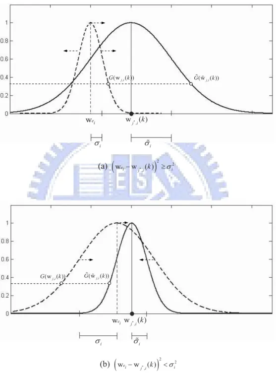
It thus covers a more fitting neighborhood region, and leads to a higher learning efficiency. With ˜G( ˜wj,i(k)), the new weight ˜wj,i(k) is derived as

˜

wj,i(k) =

|wj∗_,i(k) − w_ei(k)|

σi

· (wj,i(k) − wei(k)) + wj∗,i(k). (3.6)

And, with a desired new weight ˜wj,i(k), the learning should also make wj(k) approach

˜

w_j(k), in addition to minimizing the error function Ej(k) in Eq.(3.3). A new error function

˜

(a) *

!

2 2 ,( ) e_{i i} j i k ! " w w (b) *

!

2 2 ,( ) e_{i i} j i k ! " w w

Figure 3.4 Center and width adjustment for the neighborhood function G(wj i,( ))k ,

when (a) *

!

2 2 ,( ) e_{i i} j i k ! " w w and (b) *

!

2 2 ,( ) e_{i i} j i k ! " w w . *_,( ) j i k w i i i i e_i w , ( j i( )) G w k , ( j i( )) Gw k *_,( ) j i k w , ( j i( )) G w k , ( j i( )) Gw k e_i w

˜ Ej(k) = 1 2[(Dj− F (wj(k))) 2 ₊°°_°w j(k) − ˜wj(k) ° ° °2]. (3.7)

Based on Eq.(3.7) and the gradient-descent approach, the weight-updating rule is derived as wj,i(k + 1) = wj,i(k) − η(k) ∂ ˜Ej(k) ∂wj,i(k) = wj,i(k) − η(k)[ ∂Ej(k) ∂F (w_j(k)) · ∂F (w_j(k)) ∂wj,i(k) + (wj,i(k) − ˜wj,i(k))] = wj,i(k) − η(k)[(wj,i(k) − wj ∗_,i(k)) q · σ2 i · F (wj(k)) · (Dj − F (wj(k))) +(wj,i(k) − ˜wj,i(k))] (3.8)

where η(k) stands for the learning rate in the kth stage of learning, described in chapter 1. Together, the weight updating rule described in Eq.(3.8) and the learning rate in Eq.(2.2) will force the minimization of the difference between the weight vector of the winning neuron and those corresponding to every neuron in each learning cycle. The learning will eventually converge.

3.3

Applications

To demonstrate its capability, the SOMS is applied for both function optimization and dynamic trajectory prediction. Based on the SOMS, we first develop learning schemes corresponding to each of the applications. Simulations are then executed for performance evaluation. The results are especially compared with those of the genetic algorithm (GA) for their resemblance in searching. Both the SOM and GA have the merit of parallel processing. And, both of their searches are through the guidance of the evaluation func-tion, while the SOM in our design adopts a somewhat organized search and the GA in

some sense a random approach. It implicates that the SOM may be more suitable for applications with certain knowledge, especially when the distribution of the possible solu-tions is not utterly random. On the contrary, for applicasolu-tions with no a priori knowledge available, the GA may yield better performance.

3.3.1

Function Optimization

For a function optimization problem, the goal may be to maximize (minimize) an object function O(·). Let O(w_j(k)) be the function value for the weight vector w_j(k), which rep-resents a possible solution. The learning algorithm for function optimization is organized as follows.

Algorithm for function optimization based on the SOMS: Maximize (minimize) an object function using the SOMS.

Step 1: Set the stage of learning k = 0. Choose a reference value Pr. Estimate the

ranges of the possible parameter space and randomly store the possible parameters w_j(0) into the neurons, where j = 1, . . . , N × N, N × N the total number of neurons in the 2D (N × N) space.

Step 2: Compute O(w_j(k)) for all w_j(k).

Step 3: Among the neurons, find the one with the largest (smallest) value as the winning neuron j∗ _{for the maximization (minimization) problem.}

Step 4: Update the weight vectors of the winning neuron j∗ _{and its neighbors according}

Step 5: Check whether the difference between w_j∗(k) of the winning neuron j∗ and

w_j(k) corresponding to every neuron j is smaller than a prespecified value Pr. If it is not,

let k = k + 1, and when k is smaller than a prespecified maximum value, go to Step 2; otherwise, the learning process is completed and output the optimal value.

Two standard test functions are used to demonstrate the proposed algorithm, a 2-D Griewant function f (x1, x2) = 1 + 1 4000[(x1− 100) 2_{+ (x} 2− 100)2] − cos(x1− 100) · cos( x2− 100_√ 2 ) (3.9) and a 30-D Rosenbrock function

f (x) =

29

X

i=1

[100(xi+1− x2i)2+ (xi− 1)2]. (3.10)

These two test functions have also been used in [40]. The optimization here is to minimize these two functions. Their global minimal values are known in advance: for the Griewant function, it is 0 when (x1, x2) = (100, 100); for the Rosenbrock function, it is also 0 when

all xi are equal to 1. The SOM is chosen to be with 5 × 5 neurons and the learning rate

as

η(k) = 0.7 · e−k/50_{+ 0.2 (3.11)}

For comparison, we also use the GA for function minimization, which is with a population size of 25 to match with that of the SOM, and the crossover and mutation probability of 0.6 and 0.0333, respectively.

We start with the learning for the 2-D Griewant function. The initial w_j(0) for the SOMS was randomly chosen within the ranges of (−3, 3)×(−3, 3), i.e., the optimal solution was outside of the estimated region. Figure 3.5 shows the simulation results. In Figure 3.5(a), both SOMS and GA found the optimal minimal value successfully, while the SOMS converged faster. Figures 3.5(b) and (c) show the weight vector movement (k = 0 ∼ 11)

for the SOMS and GA, respectively. From the figures, we observed that the search in the SOMS was basically in grouping and more directional; by contrast, that of the GA was in a more random manner. It indicates that the SOMS was more effective for this 2-D Griewant function minimization, because the distribution of the possible solutions might not be utterly random.

In the minimization of the 30-D Rosenbrock function, we simulated the case that the optimal solution was within the estimated region. For its complexity, the size of the SOM was enlarged to be with 25 × 25 neurons, and that of the GA also enlarged accordingly. The learning rate for the SOMS and the crossover and mutation probabilities for the GA were set to be the same. Each wj,i(0) of the initial wj(0) was randomly chosen within

the range of (−5, 5). In addition to the SOMS and GA, the SOMO proposed in [40] was also applied for the minimization, with its parameters adjusted via a trial-and-error process to yield salient performance. Figure 3.6 shows the simulation results. In Figure 3.6, all SOMS, GA, and SOMO found the optimal minimal value successfully, while the SOMS still converged faster. It indicates that the SOMS was also effective for the 30-D Rosenbrock function minimization.

(a) Minimal function values O(w_j*( ))k during the learning process

(b) Weight vector movement in the SOM

(c) Weight vector movement in the GA

Figure 3.5 Minimization of the 2-D Griewant function using the SOMS and GA with

the optimal solution outside of the estimated region: (a) minimal function values

*

( j ( ))

O w k during the learning process, (b) weight vector movement in the SOM, and

(c) weight vector movement in the GA.

time ( ms ) 1 x 2 x * ( j ( )) Ow k 1 x

Figure 3.6 Minimal function values ( *( ))

j

O w k during the learning process for the minimization of the 30-D Rosenbrock function using the SOMS, GA, and SOMO.

time (s) (log)

*

( j( )) O w k

3.3.2

Dynamic Trajectory Prediction

For a dynamic trajectory prediction problem, the goal may be to estimate the launching position and velocity of a moving object using the measured data. Through a learning process, the SOMS may determine a most probable initial state through repeatedly com-paring the measured data with the predicted trajectories derived from the possible initial states stored in the neurons of the SOM. We consider the SOMS very suitable for this application, because the relationship between the initial state and its resultant trajec-tory is not utterly random. We can thus distribute the initial states into the SOM in an organized fashion, and make it as a guided search.

In this application, the nonlinear dynamic equation describing the trajectory of the moving object and the measurement equation are first formulated as

x(k + 1) = fk(x(k)) + ξ_k (3.12)

v(k) = gk(x(k)) + ζ_k (3.13)

where fkand gkare the vector-value function defined in Rqand Rl(q and l the dimension),

respectively, and their first-order partial derivatives with respect to all the elements of

x(k) continuous. ξ_k and ζ_k are the zero-mean Gaussian white noise sequence in Rq _and

Rl_{, respectively, with} E[ξ_k] = 0 (3.14) E[ξ_jξt k] = Qδjk (3.15) E[ζ_k] = 0 (3.16) E[ζ_jζt_k] = Uδjk (3.17) E[ξ_jζt k] = 0 (3.18)