q 2001 American Meteorological Society
The Kuroshio East of Taiwan: Moored Transport Observations from the
WOCE PCM-1 Array
WILLIAME. JOHNS, THOMASN. LEE, DONGXIAOZHANG,AND RAINERZANTOPP
Rosenstiel School of Marine and Atmospheric Science, University of Miami, Miami, Florida CHO-TENG LIU AND YIHYANG
Institute of Oceanography, National Taiwan University, Taipei, Taiwan, Republic of China
(Manuscript received 4 August 1999, in final form 12 July 2000) ABSTRACT
Observations from the WOCE PCM-1 moored current meter array east of Taiwan for the period September 1994 to May 1996 are used to derive estimates of the Kuroshio transport at the entrance to the East China Sea. Three different methods of calculating the Kuroshio transport are employed and compared. These methods include 1) a ‘‘direct’’ method that uses conventional interpolation of the measured currents and extrapolation to the surface and bottom to estimate the current structure, 2) a ‘‘dynamic height’’ method in which moored temperature measurements from moorings on opposite sides of the channel are used to estimate dynamic height differences across the current and spatially averaged baroclinic transport profiles, and 3) an ‘‘adjusted geo-strophic’’ method in which all moored temperature measurements within the array are used to estimate a relative geostrophic velocity field that is referenced and adjusted by the available direct current measurements. The first two methods are largely independent and are shown to produce very similar transport results. The latter two methods are particularly useful in situations where direct current measurements may have marginal resolution for accurate transport estimates. These methods should be generally applicable in other settings and illustrate the benefits of including a dynamic height measuring capability as a backup for conventional direct transport calculations. The mean transport of the Kuroshio over the 20-month duration of the experiment ranges from 20.7 to 22.1 Sv (1 Sv[ 106m3s21) for the three methods, or within 1.3 Sv of each other. The overall mean transport for the Kuroshio is estimated to be 21.5 Sv with an uncertainty of 2.5 Sv. All methods show a similar range of variability of610 Sv with dominant timescales of several months. Fluctuations in the transport are shown to have a robust vertical structure, with over 90% of the transport variance explained by a single vertical mode. The moored transports are used to determine the relationship between Kuroshio transport and sea-level difference between Taiwan and the southern Ryukyu Islands, allowing for long-term monitoring of the Kuroshio inflow to the East China Sea.
1. Introduction
The Kuroshio enters the East China Sea at 248N be-tween the northeast coast of Taiwan and the southern-most Ryukyu Island of Ishigaki (Fig. 1), where its mean transport has been estimated at 21–33 Sv (Sv[ 106m3 s21) from historical shipboard observations (Nitani
1972; Bryden et al. 1991; Ichikawa and Beardsley 1993; Liu et al. 1998). As it flows into the East China Sea the Kuroshio passes over the Ilan Ridge, which has a sill depth of approximately 800 m. This channel forms a natural choke point for monitoring the transport and
Corresponding author address: Dr. William E. Johns, Division of
Meteorology and Physical Oceanography, Rosenstiel School of Ma-rine and Atmospheric Science, University of Miami, 4600 Ricken-backer Causeway, Miami, FL 33146-1098.
E-mail: wjohn@rsmas.miami.edu
variability of the Kuroshio. The Kuroshio inflow through this channel feeds the main outflow of the Ku-roshio from the East China Sea through Tokara Strait and its shallow branches into the Yellow Sea and Sea of Japan. Additional inflow to the East China Sea occurs through the shallow Taiwan Strait west of Taiwan, but at a much smaller rate of 1–2 Sv (Zhao and Fang 1991). Knowledge of the Kuroshio transport entering the East China sea is important for the estimation of transpacific heat flux along 248N and for understanding the closure of the North Pacific subtropical gyre (Roemmich and McCallister 1989; Bryden et al. 1991; Hautala et al. 1994).
Shipboard section data suggests a wide range of Ku-roshio transport variation in the East China Sea from a minimum of about 15 Sv to a maximum of near 50 Sv (Nitani 1972; Guan 1981; Bingham and Talley 1991; Ichikawa and Beardsley 1993). Estimates of the mean Kuroshio transport vary from about 21 to 33 Sv. Guan
FIG. 1. Schematic of the Kuroshio and its branches in the East China Sea (after Nitani 1972), with PCM-1 array location shown.
(1981) analyzed the annual mean transports from 71 sections across the Kuroshio west of Okinawa between 1955 and 1979 and found a mean transport of 21.3 Sv with interannual variations of64 Sv. Years with strong transports occurred during La Nin˜a years and coincided with the presence of a large meander of the Kuroshio southeast of Japan. Years with weak transports occurred during strong El Nin˜o episodes in 1957–58, 63–65, and 70–71 as defined by Wyrtki (1975) and without a large meander off Japan. Akitomo et al. (1996) similarly found a correlation between the strength of the Kuroshio geostrophic transport in the ECS and the presence of the large meander off southeast Japan by comparing geostrophic transports with results from a reduced-grav-ity model of the North Pacific. They found that transport peaks on interannual timescales in the source region of the Kuroshio (178–218N) were due to intensification of the trade winds, whereas in the ECS interannual trans-port variations were caused by advection of transtrans-port anomalies from the south. Ichikawa and Beardsley
(1993) determined absolute transports from hydrograph-ic and surface current data over a 3-year period and found a mean of 23.7 6 2 Sv and an interannual var-iation of about 8 Sv.
In this paper we describe results from a collaborative Taiwan–U.S. program to measure the structure and transport of the Kuroshio as it enters the East China Sea, using a moored instrument array deployed for a 20-month period between September 1994 and May 1996. This array, named the WOCE PCM-1 array (WOCE International Project Office 1990), is the first attempt to directly measure the Kuroshio with a long-term current meter array spanning the full width and depth of the current at any location along the North Pacific western boundary. This paper is devoted pri-marily to a description of methods used for determining the Kuroshio transport and presentation of basic results on its mean structure, transport, and variability at this location. The companion paper by Zhang et al. (2001) describes further scientific results from PCM-1 on the
TABLE1. Mooring locations and instrument depths and types for the PCM-1 array deployed east of Taiwan between 18 Sep 1994 and 28 May 1996. Mooring ID Latitude Longitude Water depth Instrument depth (m) Instrument type* Duration (yyyymmdd) Record length (days) M1 248 32.259N 1228 10.199E 464 m 65 90 140 190 250 300 400 SBE16 AACM TSKA VACM SBE16 VACM VACM 19940918–19951009 19940918–19951009 19940918–19951009 19940918–19960528 19940918–19960528 19940918–19960528 19940918–19941128 387 387 387 619 619 619 72 T3 248 29.19N 1228 17.759E 452 m 390 415 ADCP SBE16 19940918–19960512 19940919–19951008 464 385 M2 248 22.399N 1228 25.19E 538 m 175 275 375 475 AACM VACM VACM VACM 19940918–19950803 19940918–19960528 19940918–19960528 19940918–19960528 320 618 618 618 T4 248 18.829N 1228 33.589E 477 m 340 380 ADCP SBE16 19940919–19950505 19940919–19960313 228 540 T5 248 14.149N 1228 43.859E 950 m 375 771 867 927 SBE16 AACM AACM TSKA 19940918–19960527 19951014–19960527 19940918–19950630 19951014–19960527 561 226 286 226 T6 248 10.089N 1228 51.429E 830 m 332 703 813 AACM AACM TSKA 19951014–19960527 19940918–19950523 19951014–19960527 226 230 226 M3 248 07.339N 1228 59.99E 595 m 75 100 150 200 250 400 594 SBE16 AACM TSKA VACM SBE16 VACM SBE16 19940919–19960527 19940919–19960310 19940919–19960527 19940919–19951205 19940919–19960527 19940919–19960527 19940919–19960527 617 539 617 445 617 617 617 M4 248 03.449N 1238 0.6869E 484 m 95 120 220 270 345 420 483 SBE16 AACM VACM SBE16 TSKA VACM SBE16 19940919–19960527 19940919–19951009 19940919–19960527 19940919–19960527 19940919–19960527 19940919–19960527 19940919–19960527 617 386 617 617 617 617 617 * Instrument types AACM: Aanderaa current meter, VACM: Vector-averaging current meter, TSKA: Temperature logger, ADCP: Acoustic Doppler current profiler, and SBE16: SeaBird CTD.
modes of Kuroshio variability and relationships to me-soscale eddy variability in the ocean interior.
The methods used herein combine both direct (based on measured currents) and indirect (geostrophically in-ferred) estimates of the volume transport. Direct esti-mation of transport using moored current meter arrays is now fairly routine and there have been many suc-cessful applications of this technique in boundary cur-rents and straits throughout the world’s oceans (Schott et al. 1988a,b; Bryden et al. 1991; Murray and Arief 1988; Lee et al. 1990, 1996; Johns et al. 1995b). For such estimates to be accurate, the mooring spacing and vertical distribution of instruments must be sufficient to resolve the basic internal scales of the velocity field and to account for possible meandering of the current if it is not tightly constrained by topography. By contrast,
indirect methods involving use of moored temperature measurements to estimate geostrophic transports have been little used even though the benefits of natural in-tegration by this technique have been recognized for some time (Stommel 1947; Zantopp and Leaman 1984). In practice, choices about moored array design are often based on limited information about the current structure or the correlation scales of the variability, and arrays are usually designed to meet the minimum requirements with little or no redundancy. Since temperature (and sometimes salinity) measurements are often collected on moorings in addition to velocity measurements, some combination of direct and indirect techniques would seem to be a useful and desirable approach to obtain robust transport estimates and to cross-check results. As we will show in this study, estimation of the Kuroshio
FIG. 2a. Plan view of the PCM-1 array and mooring locations along the Ilan Ridge.
transport by direct methods was made difficult during certain parts of the record by data gaps and losses to fishing activity, and indirect estimates provided an im-portant backup during these periods.
In the following sections we first describe the PCM-1 data and measurements (section 2) and develop and compare methods for determining the Kuroshio trans-port (section 3). Results on the mean Kuroshio transtrans-port, its vertical structure, and its range of variability and dominant timescales are given in section 4. The vertical structure of the transport fluctuations and the relation-ship between volume transport and sea level difference across the Kuroshio are also described in section 4. Section 5 contains a summary of results.
2. Measurements
The PCM-1 array consisted of a total of 11 moorings distributed along the Ilan Ridge between the east coast of Taiwan and the southern Ryukyu Island of Iriomote (Fig. 2a). We refer to this channel as the East Taiwan Channel (ETC) to distinguish it from the much shal-lower Taiwan (or Formosa) Strait lying to the west of Taiwan. Seven moorings (T1–T7) were deployed by the National Taiwan University (NTU) and National Taiwan Ocean University and four moorings (M1–M4) were deployed by the University of Miami. The mooring lo-cations and details of the instrument records are given in Table 1. The average mooring spacing was 16 km along the section (Fig. 2b). The array was designed to yield subtidal transports accurate to within62 Sv, based on experience with similar arrays in the Florida Current. The topography along the Ilan Ridge is extremely rough
and careful surveys of each mooring site were necessary to ensure proper mooring emplacement and target depths of instruments. The mooring line was placed along the upstream flank of the Ilan Ridge to minimize the potential for topographic shielding or steering of the flow as it navigates the complex channel topography.
Just downstream of the mooring line the ETC divides into two subchannels around the island of Yonaguni, with the deeper and wider subchannel being to the west (Fig. 2a). The eastern subchannel contains three shallow banks of less than 200-m depth, and any Kuroshio flow passing east of Yonaguni must either flow over these banks or through narrow channels between them with sill depths of 400–600 m. The line of moorings T1–M4 was designed to resolve the transport between the coast of Taiwan and the southernmost of these shallow banks, including most of the Kuroshio flow that could enter the eastern channel. Mooring T7 was placed in the small channel between M4 and Iriomote island to help resolve any additional flow that may enter the eastern channel east of M4.
Moorings on the west side of the channel were de-signed to measure velocity profiles from the bottom to within nominally 50 m of the surface. Moorings M1– M2 were conventional taut-wire subsurface moorings with instruments at discrete depths from 50 m to the bottom, while moorings T3, T4, and T5 contained up-ward-looking 150 kHz acoustic doppler current profilers (ADCPs) mounted at depth 350–400 m (Fig. 2b). Moor-ings M3 and M4, on the eastern side of the channel where smaller mean speeds and vertical shears were expected, had current measurements to within 100 m of the surface. Moorings T5 and T6 contained deep current
FIG. 2b. Cross section of PCM-1 moorings and instrumentation over topography. Open symbols indicate instruments that were lost or did not return data.
meters to measure the flow below 500 m entering the deep central part of the channel. The flanking shallow moorings T1, T2, and T7 were instrumented only below 100 m to reduce their exposure to heavy fishing activity in these areas. In addition to current measurements, moorings M1 and M3/M4 bracketing the main channel included extra temperature and conductivity sensors along the mooring line and precision bottom pressure gauges to allow them to function as ‘‘dynamic height’’ moorings (see section 3). All conventional current me-ters measured temperature in addition to current speed and direction, and at least one of the upper current me-ters on each mooring measured pressure to keep track of vertical mooring motion.
The array was first deployed in September 1994 from NTU’s R/V Ocean Researcher I, with servicing and final recovery from aboard the R/Vs Ocean Researcher I and
II. A time line of the status of moorings through the
experiment is shown in Fig. 3. Fishing activities resulted in complete loss of moorings T1, T2, and T7 as well as the top instruments on moorings M1 and M2. The bottom pressure sensor on mooring M1 was also lost due to a broken wire tether. Mooring T3 was retrieved and out of service from May to October 1995 and moor-ing T4 was retrieved and not redeployed after May 1995. Unfortunately no data was retrieved from the ADCP on mooring T5. Technical problems with several current meters on moorings T5 and T6 as well as some of the upper-level current meters on moorings M1 and M2 also caused a number of short or missing data records. These substantial data losses compared to that of the planned configuration required special attention to the transport calculations and to possible effects of undersampling of the cross-channel current structure.
For the transport calculations that follow, all data were edited to remove spikes and fill small gaps, low-pass filtered with a 40-h Lanczos filter to remove tidal and inertial oscillations, and subsampled at 12-h intervals. Vector (stick) plots of these low-pass filtered current re-cords are shown in Fig. 4 at the sampled depths on moor-ings M1 to M4, and at selected depths from the ADCP records on moorings T3 and T4. Mean currents and stan-dard deviations from all sites are listed in Table 2.
A detailed study of the current variability and the modes of variation of the Kuroshio observed from the PCM-1 array is given in Zhang et al. (2001), and the reader is referred there for more discussion on the var-iability. However, a few general characteristics of the fluctuations are apparent from examination of these re-cords. The current meter records from the central part of the channel (e.g., M2) tend to be relatively direc-tionally stable and are modulated by changes in intensity on timescales of several months. On the far western side of the channel (e.g., M1) the directional variability is larger with occasional reversals of the flow, and the characteristic timescales of the variability are shorter. On the eastern side of the channel (M3 and M4), the flow has considerable directional variability on the sev-eral month timescale with occasionally very strong east-ward or westeast-ward components of flow that are nearly perpendicular to the main axis of the channel.
As shown later in this paper, the modulations of cur-rent strength on several month timescales in the central part of the channel are strongly reflected in the transport variability of the Kuroshio, which has dominant time-scales of 70–100 days. The companion paper by Zhang et al. (2001) also shows that these transport variations are associated with eddy features that propagate
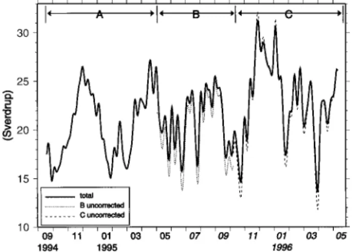
west-FIG. 3. PCM-1 mooring time line, indicating periods A, B, and C when different mooring and instrument configurations were available.
ward into the PCM-1 array region from the Philippine Sea and that these features are responsible for the large directional swings in the observed currents on the east-ern side of the array (M3 and M4) on similar timescales. The shorter timescales and brief reversals observed in the western part of the array off Taiwan are caused primarily by small-scale meanders in the path of the Kuroshio as it enters the ECS, which appear to have a much smaller impact on the transport (Zhang et al. 2001).
3. Transport calculations: Methods
Based on the available data coverage, the 20-month period of observations is broken into three segments, which we will refer to respectively as periods A, B, and C (Fig. 3). During period A, ADCP records from both T3 and T4 are available, and the transport in the western part of the section where the axis of the Kuroshio nor-mally resides is well resolved (Fig. 5). During period B, both T3 and T4 were out of service and the data coverage in the western part of the channel is provided by only M1 and M2. Period C is missing the T4 record but T3 is again available during the period. Period A therefore had the best data coverage, while period B had the worst data coverage.
Below we describe three different methods used to estimate the subtidal transport through the ETC. These
are referred to as the ‘‘direct method,’’ the ‘‘dynamic height method,’’ and the ‘‘adjusted geostrophic meth-od,’’ respectively. These methods use different combi-nations of directly measured and geostrophically esti-mated currents to determine the total transport through the channel.
a. Direct method
In the direct method, the measured currents at all available moorings are used to construct a gridded cross section of the downstream velocity component (308 True) through the channel, which is then spatially in-tegrated to yield a transport estimate. This procedure is applied at each 12-h interval to the cross section ex-tending from the Taiwan coast to the location of mooring M4. Interpolation of the measured currents along this line was carried out using triangular interpolation on a 5 km by 25 m grid with currents set to zero at the bottom and on the east coast of Taiwan. Prior to the interpolation the currents at moorings M1, M2, M3, M4, and (when available) T3 and T4, were extrapolated to the surface by extending the velocity profiles linearly to the surface using the vertical shear determined from the top two instruments. This choice was based on the observation of nearly linear (constant vertical shear) profiles from the ADCPs. Pressure measurements were included on all moorings (except T5 and T6) so that the actual
mea-surement depths are accounted for in the interpolation process. The mean downstream velocity structure de-rived for period A (Sep 1994–May 1995) is shown in Fig. 5. To close the section east of M4, a separate direct estimate of the transport between M4 and Iriomote Is-land is made that uses the component of flow along 3408T at M4 (normal to the section between M4 and Iriomote) and decreases it linearly to zero at Iriomote Island. This transport contribution, which is typically quite small (see Fig. 10), is then added to the main section transport to estimate the total volume transport entering the ETC. This transport tends to be out of phase with the transport through the main section and is largest when the Kuroshio axis shifts offshore and flows into the ETC with a northerly or northwesterly direction. The total transport time series derived from this method is shown in Fig. 6. The transports range from a low of 9 Sv to a high of about 35 Sv.
Errors or biases in the direct transport estimates re-sulting from loss of instruments during the experiment are evaluated in the appendix. It is shown there that the instrument configuration during periods B and C, when the ADCPs at sites T3 and/or T4 were absent, cause an underestimate of the mean transport and an overestimate of its variability by direct interpolation/extrapolation methods. These effects are relatively small, however, and indicate that the direct method is surprisingly robust to loss of instruments during PCM-1. To improve direct transport estimates during these periods, period A is used as a test bed to establish regressions between the transports calculated from the full array configuration and from the reduced array configurations. These re-gressions are then applied to correct the estimated trans-ports during the B and C periods. As shown in Fig. 7 by the 10-day low-pass filtered time series, the regres-sion-corrected transports are higher than the directly computed transports by about 1 Sv on average (see ap-pendix for details). The solid curve in Fig. 7 combines the directly calculated transports for period A with the regression corrected transport time series for periods B and C. This time series represents our best estimate of the Kuroshio transport and variability during the PCM-1 experiment using only the available direct current mea-surements. The mean transport is 21.5 Sv with a stan-dard deviation of 4.1 Sv and a total range of variability of the 10-day low-passed transports of 13–32 Sv.
We note that the above tests do not address other possible sampling problems with the current meter array that may cause transport errors even during period A, such as the sparse measurements in the upper 100 m and the data gap in the upper water column at moorings T5 and T6 over the deep central channel. These issues are addressed in the following sections where the direct transport estimates are compared with transports cal-culated by indirect methods.
b. Dynamic height method
The dynamic height method was developed as a means to estimate the net geostrophic transport between
widely spaced pairs of moorings to provide a backup or possible substitute for direct transport calculations. Here the method is used to estimate the Kuroshio trans-port in the upper 400 m between moorings M1 and M4, which spans the strongest part of the current and con-tains most of the total transport entering the ETC.
The steps used in creating the dynamic height trans-port estimates are as follows:
1) The temperature measurements at discrete depths on moorings M1 and M4 are combined with a local climatology of the vertical temperature gradient and sea surface temperature to create continuous tem-perature profiles from the surface to 400 m. 2) These temperature profiles are combined with
ob-served or climatological salinity values to estimate the vertical dynamic height profile at the moorings. 3) The dynamic height profiles are differenced to yield an estimate of the baroclinic transport between M1 and M4 relative to 400 m.
4) The baroclinic transport profile is referenced by the average velocity at 400 m across the width of the channel between M1 and M4 derived from the direct current measurements.
In principle all that is required for this method to work is that the temperature measurements on the moor-ings are sufficient to resolve the basic structure of the temperature profile and that the T–S relationship in the region of interest is reasonably tight. Prior to the ex-periment, tests of the method were performed on avail-able CTD casts in the ETC (from Liu et al. 1998), to evaluate sampling configurations and expected errors due to T–S variability. It was found that, for a nominal 50-m vertical spacing of temperature measurements be-tween depths of 50 m and 400 m, and use of a clima-tological T–S relation, dynamic height profiles accurate to within62 dyn cm at the surface could be reproduced using this method. The associated error in the average surface velocity between moorings M1 and M4, at a separation of 119 km, would then be of order 4 cm s21,
and the error in the baroclinic transport between them relative to 400 m would be approximately61 Sv. Moor-ings M1 and M3/M4 were thus designed with temper-ature measurements every 50 m to within 50 m and 75 m of the surface, respectively, and conductivity mea-surements were included at two depths on each mooring to provide direct salinity observations. Temperature ac-curacies for all instruments were 0.018C or better, and salinity accuracies are estimated to be 0.05 psu or better for the first 12 months of the deployment and 0.1 psu thereafter.
The methodology used to estimate continuous tem-perature profiles at the moorings follows that of Johns et al. (1995b) and Fillenbaum et al. (1997). First, cli-matological CTD data from the region are used to create an empirical function (]T/]z)(T), which specifies the mean vertical temperature gradient as a function of tem-perature (Fig. 8a). This function is combined with the
FIG. 4. Vector velocity plots of currents at moorings M1–M4 (all measurement depths), and at moorings T3 and T4 for subsampled depths from the ADCP records. Up is 308T.
measured temperatures by integrating upward and downward from adjacent measurement points on the mooring and forming a weighted average of these es-timates; namely,
z
2
T(z)5
O
w Ti[
i1E
]T/]z(T) dz ,]
i51 zi
where i 5 1, 2 are adjacent measurement levels, and where the weights wiare inversely proportional to the
vertical distance from the respective measurement
depths, wi 5 1 2 |z 2 zi|/(z2 2 z1). This procedure results in a smooth temperature profile that goes through the measured T(z) points on the mooring but which is otherwise consistent with the local mean stratification at the mooring location. Above the highest measurement level on the mooring, the integration is carried upward until either the surface is reached or the predicted tem-perature exceeds the climatological (monthly) mean temperature for that location, in which case the inte-gration is stopped and a mixed layer is added to the top of the profile at the monthly mean temperature value.
FIG. 4. (Continued )
TABLE2. Mean currents and standard deviation for all current meter records in PCM-1 array. ADCP records are shown at selected levels, subsampled at 50-m depth. All records are rotated by 308. The U component is positive toward 1208 true, and the V component is positive toward 0308 true.
Mooring ID Length (days) Depth (m) U component Mean Std dev V component Mean Std dev M1 203 619 619 72 90 190 290 390 21.4 28.5 21.2 21.3 12.8 8.1 4.9 3.6 49.5 17.1 8.0 5.2 23.8 13.6 8.6 12.7 T3 464 464 464 464 464 464 464 50 100 150 200 250 300 350 1.7 3.8 3.6 3.4 2.3 2.3 3.1 18.2 15.4 12.8 11.1 9.7 8.5 8.6 91.4 72.6 50.2 34.5 24.7 21.3 22.5 29.2 25.8 21.7 17.7 14.2 11.6 11.7 M2 100 618 618 618 175 275 375 475 29.8 0.4 2.8 11.2 8.0 8.4 6.9 5.3 57.4 39.3 23.2 12.4 11.3 11.9 9.9 4.9 T4 228 228 228 228 228 228 50 100 150 200 250 300 22.8 21.5 21.0 0.5 2.4 2.3 20.3 18.0 16.6 15.9 13.2 9.8 66.2 60.9 54.7 48.5 42.0 33.8 21.4 17.8 14.0 12.6 12.8 12.2 T5 227 286 771 867 20.623.8 3.1 2.8 2.7 21.2 3.11.8 T6 226 453 332 703 211.01.1 15.4 4.5 23.9 0.8 8.8 3.0 M3 539 443 617 100 200 400 2.6 20.1 23.0 20.9 19.4 13.1 32.2 25.7 9.3 19.9 14.6 7.7 M4 386 617 617 120 220 420 5.3 0.7 23.3 19.1 19.9 10.1 22.1 15.5 20.5 18.3 12.3 6.3
FIG. 5. Mean downstream (308T) velocity structure in the East Taiwan Channel for period A (Sep 1994–May 1995). Dots show the location of available current meter records. Coverage of the ADCP profiles is shown by heavy dashed lines.
For this application, the empirical functions (]T/]z)(T) for mooring sites M1 and M4 were determined from 11 repeat CTD stations collected near each of these moor-ings from Liu et al. (1998). Monthly mean sea surface temperatures at these sites were taken from the Reynolds and Smith (1995) climatology. Examples of estimated temperature profiles compared with actual CTD stations near the mooring sites are shown in Fig. 9.
Once the moored temperature profiles are created, climatological salinity values derived from local T–S relations (using the same set of CTD stations, Fig. 8b) are inserted and dynamic height anomaly (dD ) profiles are generated. (Incorporation of the measured salinity
FIG. 6. Kuroshio transport derived from the direct method, before application of corrections during periods B and C.
FIG. 7. Final direct method transports for the full PCM-1 period. The solid line combines the direct transports during period A with the regression-corrected transports for periods B and C. Original di-rect transports for periods B and C before cordi-rection are shown in dashed lines. Time series are filtered with a 10-day low-pass filter.
values from the few depths where conductivity was mea-sured on these moorings had little impact on these cal-culations.) The dynamic height anomaly profiles at moorings M1 and M4 are then differenced and an av-erage geostrophic velocity profile (yr) relative to 400
m is calculated for the region between the two moorings: yr(z) 5 10/ fLdD(z),
where L is the mooring separation. This relative velocity profile is referenced by adding the 400-m average ve-locity (y400) across the channel between moorings M1 and M4:
y (z) 5 yr(z)1 y400.
The reference velocity (y400) is determined at each time step by averaging the gridded 400-m velocity estimates across the channel derived from the direct interpolation. Althoughy400has its own uncertainty, it is believed to be much less sensitive to interpolation errors than higher levels in the water column due to our better overall sampling near this depth and the smaller deep lateral velocity gradients across the channel. (As an alternative to using direct current measurements distributed across the channel to reference the baroclinic transport profiles, precision bottom pressure sensors mounted at the base of each mooring could be used to monitor variations in the average reference velocity. This was our intention in this experiment, but unfortunately the bottom pres-sure sensor on mooring M1 was lost.)
Vertical integration of y (z) and multiplication by L results in an estimate of the total 0–400 m transport between moorings M1 and M4. This estimate can be directly compared to the transport between M1 and M4 over the same depth range as derived from the direct method. Since none of the direct current measurements above 400 m from M1 and M4 or the moorings in be-tween them are used in the dynamic height method, these two estimates are largely independent. To account for the areas not covered by the dynamic height method
(the shallow areas west of M1 and east of M4, and the deep central channel below 400-m depth), the direct transport estimates for these areas are simply added to the M1–M4 dynamic height transport to produce a total transport estimate.
Figure 10 shows a breakdown of the total transport derived from this method into its various components: the baroclinic transport relative to 400 m between M1 and M4, the ‘‘barotropic’’ transport between M1 and M4 (which is just y400 times the cross-sectional area between M1 and M4 above 400 m), and the transports in the shallow areas bordering M1 and M4 and below 400 m in the deep central channel. Table 4 lists the mean values and statistics of these transports. The bar-oclinic transport in the region between M1 and M4 ac-counts for slightly more than half (10.7 Sv) of the total transport through the section, and the barotropic trans-port accounts for another 5.8 Sv of the total. The var-iability is similar among the two components and es-sentially all of the longer period events are reflected in both time series. The shallow areas west of M1 and east of M4 account for only 2.1 Sv, or about 10%, of the total transport. Errors in our extrapolation of currents to these regions to estimate their transport contributions should therefore have little impact on the total transport derived in either the direct or indirect methods. The deep transport below 400 m through the M1–M4 section sim-ilarly accounts for about 2 Sv of the total transport.
Figure 11 compares the transports derived from the direct and dynamic height methods for the full length of the experiment. There is remarkable agreement be-tween the two methods for most of the record. While differences are occasionally as large as 5 Sv, the mean transport difference between the two methods is only 0.8 Sv (Table 3), and the rms difference (including the mean offset) is 3.1 Sv. The dynamic height transport tends to be lower than the direct transport during periods
FIG. 8. (a) Empirical functions (]T/]z)(T) and (b) mean T–S relations at mooring sites M1–M4 from west to east across the East Taiwan Channel. The functions are derived from repeat CTD stations near the mooring locations from Liu et al. (1998).
A and C and somewhat higher for most of period B. The lower direct transports during period B may reflect some remaining bias in the regression-corrected direct transports produced for this period (see the appendix). The lower dynamic height transports found during pe-riods A and C suggest that either the dynamic height method is underestimating the near-surface shear from its upward extrapolation of the temperature profiles, or that the direct method is overestimating the near-surface flow by its linear extrapolation to the surface. It is not obvious which method introduces this bias, and possibly both could contribute to it. However, the good agree-ment in results obtained from these two different meth-ods supports the accuracy of the direct transport esti-mates and confirms that the loss of instruments does not cause significant biases in the transport estimates over the course of the moored deployment.
c. The adjusted geostrophic method
The adjusted geostrophic method is a hybrid tech-nique that combines features of the above two ap-proaches to estimate the full field of downstream ve-locity field across the channel. This method was de-veloped to produce internally consistent fields of tem-perature and velocity across the channel for investigation of modes of variability of the current (Zhang et al. 2001). Essentially, it uses an extended application of the dynamic height method to estimate the baroclinic shear field across the entire channel. This velocity field, referenced to the observed 400-m veloc-ity, is used as a first guess of the total (geostrophic) velocity. Direct velocities are then inserted into the grid
where available and the velocity field is reinterpolated to generate a final velocity field and transport estimates. Specifically, the steps followed in the calculation are: 1) Temperature profiles are generated for the full water column at moorings M1, M2, M3, and M4 using the same procedure as in the dynamic height method. Partial temperature profiles are also generated at moorings T5 and T6 to a height of 150 m above the top instrument. These data are then interpolated onto a regular 5 km by 25 m grid across the channel using Laplacian interpolation.
2) Baroclinic velocity profiles are generated at the orig-inal mooring locations (M1, T3, M2, T4, T5, T6, M3, and M4) from the gridded temperature field with application of climatological salinities.
3) The downstream velocity at 400 m is extracted from the interpolated field of direct measurements at each mooring location and used to reference the respective baroclinic velocity profiles at each mooring. 4) Direct velocity profiles obtained from the moorings
(linearly extrapolated to the surface) are inserted in place of the estimated profiles where available. 5) The complete set of velocity profiles at each mooring
location, obtained from either direct or indirect es-timates, is interpolated onto a 5 km by 25 m grid using Laplacian interpolation with velocity set to zero at the bottom and at the Taiwan coast. The philosophy behind this method is to use the geo-strophic estimates to guide the overall structure of the velocity field where it is not well sampled by the avail-able direct measurements. For example, if the core of the Kuroshio moves offshore into the area of T5 and
FIG. 9. Comparison of estimated temperature profiles at mooring sites M1 (top) and M4 (bottom) with temperature profiles from nearby CTD stations, during PCM-1 cruises in Mar 1995 and May 1995. The bold lines are the temperature profiles constructed from the moorings, with measured temperature points shown; lighter lines are from nearby CTD stations most closely bracketing the mooring location on either side.
T6, it would be largely unresolved by the direct mea-surements and the total transport at that time would be underestimated by direct integration. The geostrophic velocity field generated through step (3) above, how-ever, would contain a representation of this structure consistent with the total transport between moorings M1 and M4 derived from the dynamic height method. (Note that the transport calculated from the geostrophic ve-locity field of step (3) is identical to the dynamic height method transport.) Thus the geostrophic method pro-vides an overall constraint on the velocity field that can help to fill in missing information from the direct mea-surements.
Substitution of directly measured velocities into the
field in step (4) will result, in general, in differences with respect to the indirectly estimated velocities and thus an inexact geostrophic balance within the section. Transport estimates obtained from the combined field may thus be either greater or smaller than that obtained from the dynamic height method. We believe, however, that it is highly preferable to use direct velocities wher-ever available due to possible errors in the dynamic height method and uncertainties in the degree of geo-strophic balance within the current. In this sense we allow the dynamic height method to function as a weak, rather than controlling, constraint on the overall trans-port and velocity structure across the channel.
FIG. 10. Time series of the total transport derived from the dynamic height method (a), and its various components: (b) ‘‘barotropic’’ (BT) and ‘‘baroclinic’’ (BC) transports between M1 and M4 (see text for definitions) and (c) transport contributions from east of M4, west of M1, and below 400 m in the central deep channel.
it reproduce the observed velocity profiles at ADCP moorings T3 and T4 during periods when they were available. In Fig. 12 we show the observed velocity time series at depths of 100 m, 150 m, and 300 m on moorings T3 and T4 in comparison with the geostrophic velocity time series derived from the indirect method through step (3) above. At mooring T3 the two time series track each other closely at 150 m and deeper, but at 100 m begin to have some significant differences on shorter timescales. Still, the agreement at low frequencies is remarkable. At mooring T4 the agreement is generally
poorer although the low-frequency events in the record also seem to be reasonably well reproduced. Note that the indirect estimate at T3 is constrained by moorings M1 and M2 that bracket it closely on either side, while at T4 it is more poorly constrained by the large sepa-ration between moorings M2 and M3. Overall the agree-ment is encouraging and suggests that the indirectly estimated geostrophic velocities offer a useful approx-imation of the real velocities. The transport time series produced from the adjusted geostrophic method is very similar to the previous two methods and shows all the
FIG. 11. Transport time series from the direct, dynamic height, and adjusted geostrophic methods for the full PCM-1 period (10-day low-passed values).
TABLE3. Kuroshio volume transports for annualized mean, total deployment length, and time periods A, B, and C.
Method Annualized mean Total 09/94–05/96 Mean Std dev Period A 09/94-05/95 Mean Std dev Period B 05/95–10/95 Mean Std dev Period C 10/95–05/96 Mean Std dev Direct Dynamic height Adj. geostrophic 21.5 20.7 22.3 21.5 20.7 22.0 4.1 4.5 4.8 20.5 18.8 19.4 3.7 3.9 3.7 21.1 22.4 23.6 3.4 4.0 4.1 23.0 21.3 23.6 4.4 4.7 5.1
same major events and large range of variability (Fig. 11). The mean transport from this method for the entire 20-month observation period is 22.0 Sv, which is 0.5 Sv greater than direct method and 1.3 Sv greater than the dynamic height method. Thus the insertion of direct velocities into the dynamic height method tends to in-crease the transport estimates. These offsets are not sys-tematic throughout the record, however. At times the adjusted geostrophic method tracks one or the other method much more closely. When there is a large dif-ference between the direct and dynamic height methods, the adjusted geostrophic transport usually tracks the dy-namic height method more closely. These periods prob-ably coincide with times when there is significant un-resolved structure by the direct method. The rms dif-ference between each of the methods is approximately 3 Sv, consistent with our expected errors for each of the methods.
4. Results
a. Mean structure and transport of the Kuroshio in the East Taiwan Channel
The mean downstream velocity structure in the East Taiwan Channel derived from the PCM-1 array shows maximum surface velocities of about 1 m s21 located
in the western part of the section near site T3 (Fig. 4). Due to meandering of the current core this value is
deeper and are thus not directly observed. However, the transports derived from the direct method using these extrapolated velocities are in good agreement with those derived from the indirect (dynamic height) method, which suggests that the extrapolated surface currents cannot be greatly in error. The subsurface velocity struc-ture displays a common feastruc-ture of western boundary currents: an offshore tilt of the velocity core with depth such that the maximum average velocities at 300 m occur near site T4 in the central channel, 40 km offshore of the location of maximum surface velocity. Near-bot-tom velocities are about 10 cm s21in both the western
and far eastern parts of the channel and decay to zero at about 800 m in the central deep channel. The average surface velocity magnitudes and overall structure of the Kuroshio shown in Fig. 5 agrees well with that derived independently by Liu et al. (1998) from repeat CTD/ ADCP transects across the PCM-1 section.
The average surface velocities of the Kuroshio in the ETC appear to be smaller than average surface velocities found in many other western boundary currents. For example, the Florida Current exhibits a maximum av-erage velocity of about 1.8 m s21 and instantaneous
surface velocities of typically 2.5 m s21(Leaman et al.
1987). This same difference was pointed out by Wor-thington and Kawai (1972) in their initial intercompar-ison of the two current systems. Part of the difference in average velocities may be explained by the 180-km-wide cross section of the ETC, which allows for large amplitude meanders of the Kuroshio to occur within the channel (Johns et al. 1995a). However, it can be seen in Fig. 4 that the northward flow of the Kuroshio nearly always extends over the entire width of the channel from M1 to M4, indicating that the instantaneous current itself
F IG . 12. Comparison of estimated downstream currents at sites T3 and T4 from the adjusted geostrophic method (dashed lines) with actual currents at these sites when available (solid lines), at depths of 100, 150, and 300 m.
FIG. 13. Transports above and below 200 m, and total transport, from the adjusted geostrophic method (10-day low-passed data).
roshio transport has shown that the three different meth-ods all yield very similar transport time series in terms of their mean values, variance, and range of variability. The mean transport obtained by averaging the results of all three methods is 21.4 Sv, which is essentially the same as the mean transport from the direct method. Therefore we take the mean transport from the direct method, 21.5 Sv, as our estimate of the mean transport of the Kuroshio for the PCM-1 observational period. The bias between methods is approximately 1 Sv, which we take as an estimate of the systematic error in this mean transport estimate. To estimate the random error in the mean transport, we first note that all of the trans-port time series exhibit a standard deviation of 4.1–4.8 Sv about their mean values (Table 3). Assuming an in-tegral timescale of approximately 2 months (due to the long timescale of dominant variability), this yields a standard error of the mean transport of approximately 1.5 Sv. Therefore our best estimate of the mean Ku-roshio transport for the 20-month duration of the PCM-1 experiment is 21.56 2.5 Sv, including probable random and bias errors.
To account for possible biases due to uneven sampling of the annual cycle, we also show in Table 3 an ‘‘annual mean’’ transport for each of the methods, which is de-fined as the average of the monthly mean transports from each method. Monthly mean transports were calculated simply as the average of all daily transport values falling within a given month over the total record length. For the PCM-1 measurement period, the months of Septem-ber–April were sampled in two years, while the months of May–September were sampled only once, in 1995. The record length averages are therefore weighted more heavily toward the months of September–April. The an-nual mean transports shown in Table 3 however are very similar to the record mean transports, differing in each case by no more than 0.3 Sv. Thus, the seasonal bias appears to be small compared to probable random and bias errors, and we take the annual mean transport of the Kuroshio entering the ECS to have the value 21.5 6 2.5 Sv. This estimate is in close agreement with Liu et al.’s (1998) mean transport estimate of 22.6 Sv at the PCM-1 section from repeat CTD/ADCP sections, and it is close to Ichikawa and Beardsley’s (1993) recent
estimate of 23.7 Sv for the mean Kuroshio transport in the ECS. It is notably smaller than some other recent estimates of the Kuroshio transport in the ECS, includ-ing those of Bryden et al. (1991), 28.3 Sv; Chen et al. (1992), 30.3 Sv; and Roemmich and McCallister (1989), 32.0 Sv. The mean transport of 21.5 Sv obtained from the PCM-1 observational period is also consistent with Guan’s (1981) long-term mean of 21.3 Sv for the years 1955–79 estimated from a large number of hydrographic sections across the East China Sea.
b. Transport variability: Timescales and vertical structure
As shown in Fig. 11 the Kuroshio exhibits very large transport fluctuations in the East Taiwan Channel with amplitudes of approximately 10 Sv, or roughly half of the mean transport of the Kuroshio through the channel. The total range of estimated transports from all three methods is 12–33 Sv for the 10-day low-passed data and approximately 9–38 Sv for the 40-h low-passed data. Previous shipboard studies have suggested a range from 15 Sv to as high as 50 Sv for the transport of the Kuroshio in the ECS (Nitani 1972; Guan 1981; Bingham and Talley 1991; Ichikawa and Beardsley 1993). There-fore, the continuous time series measurements from the PCM-1 array confirm these earlier inferences from ship-board studies of large transport variations of the Ku-roshio within the ECS.
The transport time series derived from the adjusted geostrophic method is broken down in Fig. 13 into con-tributions above and below 200 m, to illustrate the trans-port variations in layers above and below the main ther-mocline. (The results are similar for each of the meth-ods; we choose to show the adjusted geostrophic method here because it should provide the best overall estimate of variability.) For most of the major low-frequency events the transport variations are highly correlated above and below 200 m. Spectra of these transport time
FIG. 14. Variance conserving spectra of adjusted geostrophic trans-ports, for layers above and below 200 m, and total transport.
FIG. 15. Kuroshio transport-per-unit-depth in the ETC, from the adjusted geostrophic method, showing (a) mean vertical structure and standard deviation envelope superimposed on 10-day average profiles, and (b) normalized transport profiles (each 10-day profile is normalized by its vertically integrated transport value).
series (Fig. 14) show that the transport variability is dominated by fluctuations on timescales of 3–4 months (;100 days), a feature that is obvious from the time series. Secondary peaks in the transport spectrum occur at periods near 35 and 15 days. The 100-day peak ap-pears strongly in both the upper and lower layers, while the 35- and 15-day peaks are more prominent in the upper and lower layers, respectively. Thus the 100-day timescale events involve coherent fluctuations through
the entire water column while the shorter timescales appear to be less coherent in the vertical.
The causes of this variability and the three-dimen-sional structural variations that the Kuroshio undergoes as these variations occur are described in detail in Zhang et al. (2000). Here we focus on the vertical transport structure and its variability during the PCM-1 deploy-ment. The mean vertical structure of the Kuroshio has important implications for the gyre structure and me-ridional heat transport in the North Pacific, while the degree of variability in its vertical structure will affect how well the Kuroshio transport can be monitored by sea level differences across the current.
The field of downstream velocity in the channel can be integrated across the width of the channel to produce a vertical transport profile. A collection of such profiles is shown in Fig. 15a for sequential 10-day averages during the deployment period, again from the adjusted geostrophic method. The mean transport profile result-ing from the average of these profiles is strongly sheared above 500 m with a further increase in shear occurring near 200 m (Fig. 15a). Vertical integration of this mean transport profile within depth classes (Table 5) shows that nearly 40% of the transport is contained in the upper 100 m and more than 60% is contained in the upper 200 m.
A measure of the changes in relative shape of the transport profile can be obtained by normalizing the profiles by their total transport (Fig. 15b). When nor-malized in this way the individual profiles collapse onto a nearly constant shape, which indicates that the fluc-tuations have a robust vertical structure. Another way to show this is by an EOF analysis of the deviations
550–600 600–650 650–700 700–750 750–800 .800 0.14 0.10 0.06 0.03 0.02 0.03 0.65 0.43 0.21 0.10 0.01 — Total 21.96 31.51
* From adjusted geostrophic method.
of the Kuroshio at 248N in the East Taiwan Channel (PCM-1) and the Florida Current at 278N in the Straits of Florida (STACS). Florida Current data from Schott et al. (1988a).
FIG. 16. (a) 10-day profiles of deviations from mean transport profile, and (b) 1st EOF of the deviation profiles, with mean transport profile overlaid.
from the mean transport profile (Fig. 16a). The first EOF (Fig. 16b) explains 93% of the variance and its principal component time series (not shown) is nearly identical to that of the Kuroshio transport time series (Fig. 11). Interestingly, the vertical structure of this EOF is re-markably similar to that of the mean transport profile (Fig. 16b). Thus, to first order, the fluctuations scale as a simple multiple of the mean transport profile. This is perhaps not a surprising result as it suggests that similar baroclinic mode structures dominate both the large-scale
mean circulation that drives the Kuroshio and its me-soscale variability. This behavior also appears to be a feature of the Florida Current within the Straits of Flor-ida (Schott et al. 1988). The mean transport profiles of both currents are nearly linear with depth (Fig. 17), and their transport fluctuations also tend to be nearly linear with depth. However, the mean transport of the Florida Current at 278N is approximately 31.5 Sv (Leaman et al. 1987; Schott et al. 1988), which is about 10 Sv greater than the Kuroshio transport at the 248N PCM-1 section. The dominant timescales of variability are also different in the two current systems. Most notably, the energetic 100-day variability in the Kuroshio at the PCM-1 section is virtually absent in the Florida Current, presumably due to blocking effects of the Bahamas on
FIG. 18. (top) Sea level records from Keelung on northeast Taiwan and Ishigaki in the Southern Ryukyu Islands, and (bottom) their dif-ference plotted against the Kuroshio transport through the East Tai-wan Channel derived from the adjusted geostrophic method.
TABLE6. Results of linear regression of the three different transport methods against sea level difference (SLD) across the East Taiwan Channel between Ishigaki and Keelung. The regression slope indi-cates the scale factor relating total transport fluctuations (in Sv) to SLD fluctuations (in cm). Correlation coefficients for both daily av-eraged and 10-day low-pass filtered data are shown.
Transport method Correlation Daily avg. 10-day low-pass Regression slope (Sv/cm) Direct Dynamic height Adjusted geos. 0.62 0.69 0.70 0.72 0.78 0.78 0.356 .08 0.386 .07 0.416 .08
the propagation of interior mesoscale eddy signals into the Straits of Florida [see Zhang et al. (2000) for further discussion].
c. Sea level difference as an indicator of the Kuroshio Transport
An important result of the foregoing analysis is that it shows the Kuroshio has a robust vertical structure with regard to its fluctuations. This means that it should be possible to monitor variations in the Kuroshio trans-port through the ETC quite accurately with sea level differences across the current. The sea level difference across a current provides a measure of the average sur-face geostrophic velocity, ys5 g/fLDh, where Dh, is
the absolute sea level difference over width L of the current. The accuracy with which the sea level differ-ence can determine the transport thus depends on how closely the average surface current and total transport are related. The scale factor relating sea level difference and transport variations similarly depends on the par-ticular structure, or shape, of the vertical transport pro-file. Using the profile in Fig. 16b that is derived from the PCM-1 mooring data, we can estimate the expected scale factor for the Kuroshio in the ETC. The result is 0.35 Sv/cm; that is, the mooring data suggest that for each 1 cm increase in absolute sea level difference
across the current, the corresponding total transport should increase by approximately 0.35 Sv.
Sea level records during the period of PCM-1 are available from two long-term tide stations on either side of the ETC: in Keelung on the northeast coast of Taiwan and from Ishigaki in the southern Ryukyu Islands (Fig. 1). Other sea level records (discussed in Yang et al. 2000) are available for the western (Taiwan) side of the current during PCM-1, but we will restrict our attention here to Keelung as it provides the longest historical record suitable for monitoring sea level on the western side of the current. The two sea level records, after removal of inverted barometer effects at each site, are shown in Fig. 18a. The time series of sea level difference across the ETC between these stations, relative to a zero mean, is shown in Fig. 18b, together with the moored transport derived from the adjusted geostrophic method. There is clearly a good correlation between the sea level difference and the volume transport, especially for the longer period events. Some obvious discrepancies are also evident, for example, in February–March 1995 and again in January 1996. These events are shown in Zhang et al. (2000) to coincide with periods when the Kuroshio was strongly interacting with offshore eddies from the Philippine Sea, causing large meanders to develop in the Kuroshio just upstream of the PCM-1 section. These intense interactions may have perturbed the geostrophic balance across the section or caused the normal rela-tionship between sea level difference and transport to break down during these periods.
Regression of the sea level difference time series against the transports derived from each of the three methods yields the results shown in Table 6. For daily averaged transports, the correlations range from 0.62 for the direct method to 0.70 for the adjusted geostrophic method. For 10-day low-passed values these correla-tions improve to 0.72 and 0.78, respectively. The scale factor (regression slope) relating the fluctuations in transport and sea level difference ranges from 0.35 to 0.41 for the different methods, comparable to the pre-diction from the moored data. These values are also very similar to the results derived for the Florida Current by Maul et al. (1990), which showed a correlation of ap-proximately 0.7 between sea level difference and
trans-variability over a 20-month period from September 1994 to May 1996.
Three methods are developed to determine the volume transport that use different combinations of directly measured and geostrophically estimated currents across the moored section. These methods all produce similar transport time series and yield a robust estimate for the mean Kuroshio transport at this location of 21.56 2.5 Sv. The indirect methods, based on geostrophically es-timated currents, are shown to provide a useful backup for direct transport estimation during periods when in-strument losses or failures caused significant gaps in the spatial coverage of the array. The simplest of these methods, which we call the dynamic height method, determines the geostrophic transport between the end-point moorings along the section through the use of multiple temperature (and optionally conductivity) sen-sors distributed on the moorings. The resulting spatially averaged, geostrophic velocity profile between the end-point moorings can be referenced by precision bottom pressure gauges on the moorings or, in the present case, by using spatially averaged deep currents measured across the moored section. This is a potentially powerful and cost effective technique for making long-term mea-surements of important currents systems in the World Ocean when only the total transport and integrated ver-tical structure of the current are needed.
The Kuroshio at the 248N PCM-1 section is found to exhibit large transport variations of 610 Sv on time-scales of several days to months. The dominant transport variations occur on 3–4 month (;100 day) timescales and are related to mesoscale ocean eddy features that propagate into the western Philippine Basin and strongly influence the Kuroshio off the east coast of Taiwan (Zhang et al. 2000). Seasonal variation of the Kuroshio at this location appears to be small in comparison to these mesoscale fluctuations, and a longer record than is available from this 20-month measurement period will be needed to resolve it. The large transport variations found at the PCM-1 section are consistent with previous indications of large transport variability of the Kuroshio in the East China Sea from shipboard studies and verify that these transport variations are real and not an artifact of sampling or referencing uncertainties.
al. 1994). The strong overturning cell in the Atlantic contributes approximately 13 Sv to the transport of the Florida Current above its wind-driven component (Schmitz and Richardson 1991), while in the Pacific only about 3 Sv of the Kuroshio may be attributed to a thermohaline component that takes part in North Pa-cific Intermediate Water formation (Talley 1993). The Florida Current transport of 31.5 Sv thus carries about 80% of the combined northward wind-driven gyre and thermohaline return flows in the Atlantic (;40 Sv), while the Kuroshio transport of 21.5 Sv in the ETC appears to account for only about 60% of the combined flows in the Pacific (;37 Sv). In both cases a significant northward western boundary flow of order 10 Sv is implied in the region seaward of the Bahamas and the Ryukyu Islands, respectively, to balance the net gyre and thermohaline circulation budgets (Schmitz et al. 1992; Hautala et al. 1994; Lee et al. 1996).
Finally, we show that the detailed time series mea-surements made along the PCM-1 section provide a means to check and calibrate methods for long-term monitoring of the Kuroshio transport in the East China Sea. Analysis of the vertical structure of the transport variations from the PCM-1 array shows that these trans-port variations have a robust vertical structure similar in shape to the mean vertical transport profile of the Kuroshio. This robust vertical structure means that es-timates of the surface transport (or mean surface ve-locity) across the Kuroshio should be closely correlated with total transport variations. Analysis of sea level re-cords from Keelung on northeast Taiwan and Ishigaki in the offshore Ryukyu Islands shows that their sea level difference is correlated with transport through the PCM-1 section at a level of 0.70 for daily transports and 0.78 for 10-day averaged transports. Records from these stations date back to the 1960s and permit inves-tigation of the climatological seasonal cycle of the Ku-roshio as well as its interannual variability. Shorter term sea level records from the east coast of Taiwan closer to the PCM-1 section, analyzed by Yang et al. (2000), may provide an even better western endpoint for Ku-roshio transport monitoring. Thus, sea level differences appear to hold great promise for long-term monitoring of the transport variability of the Kuroshio near the
FIG. A1. Mean downstream velocity cross sections for period A, derived from (a) the full available mooring configuration, and for reduced configurations (b) without mooring T4 and (c) without moor-ings T3 and T4. The associated transport time series for these con-figurations are shown in Fig. A2.
PCM-1 section. Monitoring of the Kuroshio at this im-portant choke point between Taiwan and the southern Ryukyu Islands will likely be valuable for many long-term studies, including understanding of gyre responses to wind forcing, interannual variability of meridional ocean heat transport in the subtropical Pacific, and the nature of extratropical responses to El Nin˜o.
Acknowledgments. Funding for the collection and
analysis of this data was provided jointly by the U.S. National Science Foundation under the auspices of the U.S. WOCE Program (NSF Grants OCE9302187 and OCE98185672) and by the Taiwan National Science Council. The assistance of the captain and crew of the Taiwan R/V Ocean Researcher I and II in the field op-erations is gratefully acknowledged. Technical assis-tance in the mooring operations was provided by M. Graham, R. Jones, and D. Troutman of the University of Miami’s Ocean Technology Group, under the direc-tion of P. Bedard. We thank J. Overton and J. Carpenter for their assistance in word processing and figure prep-aration for the manuscript.
APPENDIX
Effects of Array Configuration on Direct Transport Estimates
In this appendix we evaluate the sensitivity of the direct calculations to the varying measurement resolu-tion during the experiment and develop a correcresolu-tion to be applied during periods B and C when data gaps are shown to lead to small biases in the direct transport estimates. Period A, with the best coverage, is used to test the other periods B and C by 1) subsampling the full mooring configuration to the available configuration during those periods and 2) recomputing the transport using the same interpolation and extrapolation tech-niques as described in section 3, direct method. The results of the tests are illustrated in Figs. A1 and A2 and Table A1. The main results are:
1) The mean current structure derived for the reduced array configurations agrees quite closely with that for the full period A configuration (Fig. A1). The only notable difference is the poorer representation of the mean Kuroshio core by undersampling of the shear zones on either side of the core by the reduced arrays.
2) For both reduced array configurations, the mean transport is slightly underestimated due to these un-dersampling effects. The loss of mooring T4 (period C) leads to an underestimate of the mean transport by 0.8 Sv in period A, while the loss of both moor-ings T3 and T4 (period B) leads to an underestimate by 1.3 Sv (Table A1).
3) The transport variability is slightly overestimated by the reduced arrays (Table A1), which appears to be
mainly a result of underestimation of the transport during low transport events (Fig. A2).
From these tests we conclude that biases introduced into the direct transport calculations by loss of instruments during the experiment are not large, of order 1 Sv, and that in terms of mean transport the direct method is
FIG. A2. Direct method transports for period A, calculated using the full array configuration [curve (a), bold line], without T4 [curve (b), light line], and without moorings T3 or T4 [curve (c), dashed line].
TABLEA1. Volume transports from different instrument configurations during period A (Sep 1994–May 1995). Configuration Mean Std dev Min Max All data Without T4 Without T3/T4 20.5 19.7 19.2 3.7 4.2 4.1 11.9 8.7 6.4 29.9 30.4 30.0
surprisingly robust to these losses. Instantaneous trans-port estimates may however have errors of up to 3–5 Sv due to the reduced coverages available in the later periods of the experiment.
To attempt to account for these biases in mean trans-port and amplitude of variation introduced by the re-duced array configurations, linear regressions were per-formed between the full array and reduced array trans-ports calculated from period A (Table A2). Assuming these regressions hold approximately for the other pe-riods, they can be used to grossly correct the direct transport estimates for these periods. We do not expect these corrections to accurately reproduce details of the transport variability during these other periods; rather, they are an attempt to account for biases in the mean transport and dominant (low-frequency) variability. Ap-plication of these regressions to the B and C periods, respectively, results in a mean increase of 1.2 Sv for the B period and 0.4 Sv for the C period compared to the conventional direct transports for these periods, and an associated decrease in the range of the fluctuations (see Fig. 7). The final direct method transport time series is then created by combining the direct transport esti-mates for period A with the regression-corrected trans-ports for periods B and C as calculated above. This time series is shown in Fig. 7 of the paper and is used for all subsequent calculations in the paper regarding mean transports and variability derived from the direct meth-od.
port using an inverse technique. Deep-Sea Res., 38, 521–545. Bryden, H. L., J. Candela, and J. T. Kinder, 1990: Exchange through
the Straits of Gibraltar. Progress in Oceanography, Vol. 33, Per-gamon, 201–248.
, D. H. Roemmich, and J. A. Church, 1991: Ocean heat transport across 248N in the Pacific. Deep-Sea Res., 38, 297–324. Chen, C., R. C. Beardsley, and R. Limeburner, 1992: The structure
of the Kuroshio southwest of Kyushu: Velocity, transport and potential vorticity fields. Deep-Sea Res., 39, 245–268. Fillenbaum, E. R., T. N. Lee, W. E. Johns, and R. Zantopp, 1997:
Meridional heat transport variability at 26.58N in the North At-lantic. J. Phys. Oceanogr., 27, 153–174.
Guan, B., 1981: Analysis of the variations of volume transports of the Kuroshio in the East China Sea. Proc. Japan–China Symp.
on Physical Oceanography and Marine Engineering in the East China Sea, Special Report of Institute of Ocean Research,
Shi-mizu, Japan, Tokai University, 118–137.
Hautala, S. L., D. H. Roemmich, and W. J. Schmitz Jr., 1994: Is the North Pacific in Sverdrup balance along 348N? J. Geophys. Res.,
99, 16 041–16 052.
Ichikawa, H., and R. C. Beardsley, 1993: Temporal and spatial var-iability of volume transport of the Kuroshio in the East China Sea. Deep-Sea Res., 40, 583–605.
Johns, W. E., T. N. Lee, C.-T. Liu, and D. Zhang, 1995a: PCM-1 array monitors Kuroshio transport. WOCE Notes, 38(3), 10–13. [Available from U.S. WOCE Office, Department of Oceanog-raphy, Texas A&M University, College Station, TX, 77843-3146.]
, T. J. Shay, J. M. Bane, and D. R. Watts, 1995b: Gulf Stream structure, transport, and recirculation near 688W. J. Geophys.
Res., 100, 817–838.
Leaman, K. D., R. Molinari, and P. Vertes, 1987: Structure and var-iability of the Florida Current at 278N: April 1982–July 1994.
J. Phys. Oceanogr., 17, 565–583.
Lee, T. N., W. E. Johns, F. Schott, and R. Zantopp, 1990: Western boundary current structure and variability east of Abaco, Ba-hamas at 26.58N. J. Phys. Oceanogr., 20, 446–466.
, , R. Zantopp, and E. Fillenbaum, 1996: Moored obser-vations of western boundary current variability and thermohaline circulation at 26.58N in the subtropical North Atlantic. J. Phys.
Oceanogr., 26, 962–983.
Leetmaa, A., P. P. Niiler, and H. Stommel, 1977: Does the Sverdrup relation account for the mid-Atlantic circulation? J. Mar. Res.,
35, 1–10.
Liu, C. T., S. P. Cheng, W. S. Chuang, Y. Yang, T. N. Lee, W. E. Johns, and H. W. Li, 1998: Mean structure and transport of Taiwan Current (Kuroshio). Acta Oceanogr. Taiwan, 36, 159– 176.
Maul, G. A., D. A. Mayer, and M. Bushnell, 1990: Statistical rela-tionships between local sea level and weather with Florida–Ba-hamas cable and Pegasus measurements of Florida Current vol-ume transport. J. Geophys. Res., 95, 3287–3296.
through the Lombok Strait, January 1985–January 1986. Nature,
333, 444–447.
Nitani, H., 1972: Beginning of the Kuroshio. The Kuroshio, H. Stom-mel and K. Yoshida, Eds., University of Washington Press, 129– 163.
Reynolds, R. W., and T. M. Smith, 1995: A high-resolution global sea surface temperature climatology. J. Climate, 8, 1571–1583. Roemmich, D., and T. McCallister, 1989: Large scale circulation of the North Pacific Ocean. Progress in Oceanography, Vol. 22, Pergamon, 171–204.
Schmitz, W. J., and P. L. Richardson, 1991: On the sources of the Florida Current. Deep-Sea Res., 38 (Suppl. 1), S379–S409. , J. D. Thompson, and R. J. Luyten, 1992: The Sverdrup cir-culation for the Atlantic along 248N. J. Geophys. Res., 97 (C5), 7251–7256.
Schott, F. A., T. N. Lee, and R. Zantopp, 1988a: Variability of structure and transport of the Florida Current in the period range of days to seasonal. J. Phys. Oceanogr., 18, 1209–1230.
, M. Fieux, J. Kindle, J. Swallow, and R. Zantopp, 1988b: The boundary currents East and North of Madagascar. 2. Direct mea-surements and model comparisons. J. Geophys. Res., 93 (C5), 4963–4974.
Stommel, H., 1947: Note on the use of T–S correlation for dynamic height anomaly computations. J. Mar. Res., 6, 85–92. Takematsu, M., K. Kawatate, W. Koterayama, T. Suhara, and H.
Mit-suyasu, 1986: Moored instrument observations in the Kuroshio south of Japan. J. Oceanogr. Soc. Japan, 42, 201–211. Talley, L. D., 1993: Distribution and formation of North Pacific
In-termediate Water. J. Phys. Oceanogr., 23, 517–537.
WOCE International Project Office, 1990: WOCE PCM1 Design Workshop, Shimizu, Japan, Tokai University, WOCE Rep. 57/ 90, 24 pp.
Worthington, L. V., and H. Kawai, 1972: Comparison between deep sections across the Kuroshio and the Florida Current and Gulf Stream. Kuroshio: Physical Aspects of the Japan Current, H. Stommel and K. Yoshida, Eds., University of Tokyo Press and University of Washington Press, 371–385.
Wyrtki, K., 1975: El Nin˜o—The dynamic response of the Pacific Ocean to atmospheric forcing. J. Phys. Oceanogr., 5, 572–584. Yang, Y., C.-T. Liu, T. N. Lee, W. E. Johns, H. W. Li, and M. Koga, 2000: Sea surface slope as the estimator of the Kuroshio volume transport east of Taiwan. Geophys. Res. Lett., in press. Zantopp, R. J., and K. D. Leaman, 1984: The feasibility of dynamic
height determination from moored temperature sensors. J. Phys.
Oceanogr., 14, 1399–1406.
Zhang, D., W. E. Johns, T.N. Lee, C.-T. Liu, and R. Zantopp, 2001: The Kuroshio east of Taiwan: Modes of variability and rela-tionship to interior mesoscale eddies. J. Phys. Oceanogr., 31, 1054–1074.
Zhao, B., and G. Fang, 1991: Estimate of water volume transports through the main straits of the East China Sea. Acta Oceanol.