The impacts of synchronized and non-synchronized reception on broadcast in multihop radio networks

National Radio Science Conference,

NRSC’99

Ain Shams University, Feb.

23-25,1999,

Cairo, Egypt

I

=

]

The Impacts of Synchronized and Non-synchronized Reception on Broadcast

in Multihop Radio Networks

Kuang-Hung

Pan’,

Hsiao-Kuang Wu’, Rung-Ji Shang3, and Feipei LailP3

‘Dept. of Electrical

Eng., National Taiwan University, Taipei, Taiwan

kpan@ archi.csie.ntu.edu.tw, flai @cc.ee.ntu.edu.tw

2Dept. of Computer Sci.

and

Information Eng., National Central University, ChungLi, Taiwan

hsiao @csie.ncu.edu. tw

3Dept. of Computer

Sci.

and

Information Eng., National Taiwan University, Taipei, Taiwan,

shang @ archi.csie.n tu. .edu. tw

Abstract

If the time lag between collided packets is small on the order of a symbol, the reception is synchronized;

otherwise, the reception is non-synchronized. We find that there is a time complexity gap exponential with the

degree of the network between the performance of synchronized and non-synchronized reception.

I.

Introduction

Broadcast is

an

important task in distributed computing and systems, It can be used for disseminating information among a set of receivers [l], and exchanging messages in distributed computing [2]. In single-hop wireless networks with a base station, such as cellular networks, broadcast can be done by sending a message from the base station to every mobile user in the down-link channel [3]. In a multihop wireless network, there is not a base station that can communicate with all users directly, and not all users can receive the messages from all other users directly [I]. Therefore, it is not so simple to solve the broadcast problem in a multihop wireless network. Modern applications of such multihop networks include disaster recovery, e.g., search and rescue in fire or earthquake and ad-hoc personal communications networks, which could be rapidly implemented, e.g., on a campus, to support collaborative computing and provide access to the Internet during special events like concerts and festivals 14-71.

Numerous researches have been conducted to investigate the broadcast problem in mul tihop wireless network. Chlamtac and Weistein proposed a centralized broadcast algorithm with time complexity O(RlogzV), where R is the radius of the network, and V is the number of mobile users in the network [8]. Broadcast protocol based on multi- cluster architecture [9] was proposed in [lo]. In [ll], it was proved that any broadcast algorithm requires Ln(logzV)

time slots to finish for a radius-2 network. In 1121, it was proved that any distributed broadcast algorithm requires Q(RlogV) time slots to finish. Bar-Yehuda, Goldreich, and Itai in [13] proposed a distributed randomized algorithm, which needs only O((R+ZogV/&)logV) time slots to finish with probability I-&. This algorithm is exponentially superior to any distributed deterministic algorithm, which takes o(V) time slots even for a radius3 network. Based on this randomized algorithm, a routing and multiple-broadcast algorithm was proposed in [141. In [lSl, an Q(Dlog(V/R)) lower bound for randomized broadcast algorithm was provided by Kushilevitz and Mansour.

Besides, more considerations should be taken to better describe the real environment in modem and coming wireless networks. In the previous work [16], the issue of channel reliability was introduced to take into account the variations

in power levels in the performance analysis of broadcast.

In this paper, we analyze the performance of broadcast with more considerations than those in [17]. The impact of the time lag at symbol (bit) level between collided packets is analyzed. If the time lag between packets is small, we

National

Radio

Science Conference,

NRSC'99

Ain Shams University, Feb. 23-25, 1999,

Cairo,

Egypt

I

C24

I

2

I

Related research topics appear in the analysis of single-hop networks. The phenomenon that a collision does not necessarily destroy packets is called capture [2][18][19]. Capture could enhance the p e r f o m c e of random access protocol radio such as ALOHA, and capture influences the performance of CDMA (code division multiple access) [19]. The goal of the MAC (medium access control) in those topics is to achieve multiple access. Therefore, the packets involved in a collision have different contents. The broadcast problem here contains only single message, therefore, it is successful

as

long

as

at least one packet is received successfully. Thus, the goal of MAC is to carry this packet to all users. Besides, the network here is multi-hop, so the packet has to be transmitted hop by hop to reach every user. Therefore, the packets involved in a collision have the same contents, if the packets are broadcast in ordered sequence.

In this paper we analyze the performance of broadcast with synchronized and non-synchronized reception in multihop radio networks. We examine the performance gap between them. How to adjust the parameters in the

broadcast algorithm to achieve better performance i s also investigated. The rest of the paper is organized

as

follows. Section II analyzes the probability of successful reception of a packet. Performance of broadcast algorithms is analyzed in section

DI.

Section

N

gives numerical examples and discussions. Conclusions are provided in section V.

U.

Probabilities

of

Successful

Reception

Synchronization can refer to that at carrier phase, bit, word [20][21], or algorithm 1221. The definitions of

synchronized and non-synchronhed reception in this paper are as follows. If the time lag between simultaneo~ly- received packets is small enough in comparison with the duration of a symbol (bit), the reception is called

synchronized. In the following, it is assumed that every slot is designed to contain a guard period [ 191 to allow all

the paths to arrive in a slot duration. Thus, the packets in previous slots do not interfere with the packets in the current slot.

In this paper, it is assumed that the time lag between components from the multi-paths 1191 is within a symbol interval, and the sum of their amplitude is Rayleigh distributed 1191. Equivalently, their power level is exponentially distributed 119,20211. Incoherent binary FSK is used for modulation and demodulation [20,21].

Here we are going to analyze the probability of successfid reception of a packet. Assume the average energy per

bit [20] for each received packet is Eb. The power level of the Gaussian noise at the receiver is

No.

We assume the fading is slow 1193. Thus, if one bit is not received successfully, it probably

means

the fading is quite severe for the whole packet containing the bit, and the packet is unlikely to be received successfidly. Therefore, analyzing bit error

probability is

an

approximate of the probability that a packet can be received successfully. The probability of bit error for incoherent binary FSK in a Rayleigh fading channel is

pb= 1 / ( 2 +

z),

(2.1)

where ;is the average signal-to-noise ratio [20], 1211. To analyze the relation between time lag and the probability of

successfully reception, we can use the formula of probability of error for incoherent binary FSK [20]:

Given z, the time lag, Tb, the bit duration,

W I ,

average power level of packet 1, W,, average power level of packet 2,

0, the phase difference between packets 1 and 2, and

No,

the average noise power, we can calculate the probability of error in a manner similar to the approach in 1201. Numerical examples will be given in section

IV.

In the following, we are going to analyze the relation between the number of packets received and the probability of successful reception with synchronized and non-synchronized reception.

In the case of synchronized reception, i.e., the time lag between the packets is small enough, the output is the sum

of the individual components transmitted from each processor. Since each packet contains the same symbols (bits), the sum of the simultaneously arriving packets has the same symbol (bit) sequence as each packet. For most of the

time, the signal simultaneously received can be viewed as constructive interference.

Denote the number of packets arriving at the same time as n. With Rayleigh fading, the in-phase and quadri-phase components of the interfering signal are Gaussian random variable [19,20,21]. Since the sum of Gaussian random variables is a Gaussian random variable with variance equal to the sum of the components of it 119, 20, 211.

Therefore, the average energy per bit of the sum of all received packets is n*Eb because each packet has the same

symbol - sequence and the reception is synchronized. Thus, the probability of bit error has the same form

as

(3. l), and In the case of non-synchronized receprion, the signals simultaneously received can be viewed

as

destructive interference for most of the time. That is, the signals from other packets are only interfering as noise. With Rayleigh fading, the power level of the sum of the interfering signds can be calculated as (n-1)*~~, and

Z=

Ed(NO+(n-1)&,).

16th

National Radio Science Conference, NRSC’99

Ain

Shams University, Feb.

23-25,

1999,

Cairo,

Egypt

m

-

j

III.

Performance of

Broadcast Algorithms

System Model

The network is represented by an undirected graph G, in which a node denotes a mobile user and an edge between

two nodes means that these two nodes are connected. The degree of a node is the number of neighbors this node has. The degree D of the network is the maximum degree of the nodes. The radius R of the network is the maximum number of edges in the shortest path between any two nodes. The probability that a processor is so busy with other tasks that it temporarily does not execute the algorithm is also included. This may result from some emergent event that a processor has to deal with, or power-saving considerations with lightweight processors, etc. Allowing the processors not to carry out broadcast temporarily enables the processors to deal with other urgent task or to save power. All processors are assumed to have the same characteristics, and are dedicated to executing the algorithm in a time slot with the same probability pr.

Broadcast Algorithm

The goal of a broadcast algorithm is

to

let as many users in the network as possible to receive a message successfully. Each user in the network executes the broadcast algorithm.

Centralized and deterministic broadcast algorithms were shown that they do not perform well in multihop wireless networks. Instead, randomized broadcast was shown to be able to fulfill the task in bounded time [16]. Therefore, a

more practical approach to fulfilling the task of broadcast is a distribured and randomized algorithm [ 171. In this paper, we choose the randomized distributed algorithm in [ 131 for the performance analysis of distributed

randomized algorithm. In this algorithm, any mobile user receiving the message to be broadcast in this time slot will broadcast the message at the next time slot. To prevent the situation that too many nodes are transmitting and collisions of packets

are

too frequent, the algorithm uses a procedure called “Decay”. In the “Decay”, a processor that is transmitting at this time-slot may stop or continue transmitting at the next time slot with a specified probability (this probability will be abbreviated as q), This process repeats for

rzl

time slots. In the following, m denotes the message

to

be broadcast.

P r o c e d u r e Decay

i z l ,

m ) ;

repeat at most

rz1

times (at least once)

transmit m to all neighbors;

exit with probability 1-q;

The whole randomized algorithm uses

rzl

as the number of time slots in a stage, i.e. the transmitting processors restart executing “Decay” every

r d

time slot 1131. In time slot 0, a processor, called the source, generates and broadcasts the message m to other users. Then every processor executes the following broadcast procedure.

P r o c e d u r e Broadcast;

Wait until receiving the message m ;

do T times

Wait until (Time mod

rd)

=O;

mca&l,

m ) ;

e n d d o .

For the situation where a sequence of packets have to be broadcast, the above algorithm can serve as one step in a

comprehensive algorithm, in which the packets are broadcast in an ordered sequence.

Performance of broadcasting

The algorithm used in both the cases of synchronized and non-synchronized reception is the same. The difference relies on the system parameters

rd.

Consider the situation in which there are n neighbors trying U, broadcast the message m to user i at time slot 0. Let f l q t ) denote the probability that i receives m before time t from one of the n transmitting neighbors. As in [14],

Procedure

Broadcast

uses

rzl

as the number of time slots in a stage, i.e., the processors restart executing “Decay” every

rzl

time slot. Since the maximum value of degrees is D, i.e. the upper bound of n is D, we choose

rzl

a minimum value such thatfTD,rzl)L P,. Therefore, the difference in performance of synchronized and non-synchronized reception can be known by the analysis of fln,t) in each case. Thus, in the following paragraphs,fln,t) will be analyzed.

The recurrence relation [23,24] of the probability that i receives m before time t from one of the n transmitting neighbors (denoted asf(n,t)) is

ldh

National Radio Science Conference,

NRSC'99

Ain

Shams University, Feb.

23-25,1999,

Cairo,

Egypt

p i l - 2 - l

where Psc,.ess[n] represents the probability that i receives m successfully in the 0th time slot, i.e., the probability that the packet is successfully received under the condition that n packets are received at the same time, and in the term (1

- PmmCJn]) c C l , , j &l- q)"+f(j, f-1), (1 - Pmccs[n]) is the probability that i does not receive m successfully in

the 0th time slot, and Cwd( 1- q)n-i represents the probability of occurrence of j neighbors keeping transmitting in the next time slot, which is multiplied by fi,t-l), the probability of successful reception for each case. The probability P,m.fJn] for synchronized reception and non-synchronized reception can be calculated from the analysis in the previous section a9follows. Taking the probability that a processor is taking a rest into account, the probability that a user receives a packet successfully is

11

I=o

I1

Psccess[nl = (l-pr)*

Cc1,.j

(l-pr)jp,'"J' ~ r c c e i v e h l , (3.2)

where (1-p,) is the probability that the receiving node is not taking a rest, C,l-p,)j p/" represents the probability that j neighbrs are not taking a rest and are transmitting the packet in this time slot, and Pmceived[j] is the probability that a packet can be received correctly in a collision of j packets. PrrMivadjj = j( l-pm) il, where paJ is the probability that a interfering packet becomes non-synchronized with desired packet.

IV.

Numerical Examples

and

Discussions

As indicated in sections I and II, in a network G, the physical environment and the design of working power determine the network topology and the parameters R, D. There seems a tradeoff between D and R. If the transmitters increase their power levels, R could decrease and D could increase. Therefore, evaluating the performance of the broadcast algorithm is very helpful not only in saving time but also in increasing power efficiency. By the result of [14], it seems that minimizing the time complexity requires minimizing R and D. Besides, from the result inT171, different retransmission probability (q) also influences the p e r f a m c e a lot. How to decide an optimum value depends on the values offln,t) and

rd,

Based on their importance, we are going to give numerical examples offln,f) and

rzl

in this section. And this optimization problem will be examined later in this section. Before that, we evaluate equation (3.1) using recursive method [23,24]. First of all, we have to evaluate

Pnceivcdn],

the probability that the packet is received correctly; then can we analyzRJTn,t) by (3.1); then r T 1 is obtained as a minimum value such that

Relation between time lag and probability of successful reception

Prccervedlfl can be obtained from the analysis in the previous section. If Hamming coding 1201 is used for e m r correction, the probability of successful reception is calculated as

P,,,,,,d/jl= (( 1-Pb)7+Pb( i - ~ b ) ~ ) ~ ~ , where L is the length of the origina~ message without error correction coding, and

Pb is the probability of bit error. For incoherent binary FSK in a collision of two packets with Rayleigh fading, Pb =

1/(2+

i-1,

where Zis average signal-to-noise ratio = Eb(l+(Tb-Td/Tb)/(No+ TImb), Eb is energy per bit,

N~

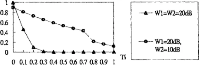
is noise level, Tb is bit duration, and TI is time lag between the two packets.

In Fig. 1, the relation between the probability of successful reception and the time lag is plotted. The contents of the two simultaneous received packets are the same, since it is assumed that the users broadcast a packet at a time. Denote the power level of the two packets by

W l

and

W2,

respectively. For the

case

of the same packet power

(Wl=W2=20dB), the probability of successful reception decreases with the time lag increasing. For time lag =1, i.e., time lag = symbol duration, the probability of successful reception is almost zero. The situation for time lag >I is not plotted because the probability of successful reception does not vary too much from time lag = 1. Therefore, we can say that the reception begins to be non-synchronized after about time lag = 0.2 for the case of

W,

= W2 = 2Od.E. With

time lag increasing, the probability of successful reception can be raised only by raising the signal to interference ratio, as the Wl=16dB, W2=10dB curve in Fig. 1, since the interference is destructive. For synchronized reception, the

probat~ility of success~l reception for W1=Wy=20dB is larger than that for W1=20dB, W2=10dB because the interference is constructive.

Probability of successful reception with n packets simultaneously received Pmd,.&n] for different cases

The influences of synchronized and non-synchronized reception on Pmceivcd[n] were analyzed, and we obtain the numerical examples. We have the following observations from the numerical results in Fig. 2, where pN is the

probability of a packet being non-synchronized received.

Then, it can be seen that PrrCei,&] decreases more quickly with pm (the probability of being non-synchronized) increasing. That means, with the probability of being non-synchronized reception increasing, the probability of fTD,rz-l)z

P,.

16‘h

National Radio Science Conference, NRSC’99

Ain

Shams

University, Feb.

23-25, 1999,

Cairo, Egypt

-1

successful reception decreases. This stems from the phenomenon that for Synchronized reception, simultaneous reception of more than one duplicate of the same packet results in better performance. For non-synchronized reception, the interfering packets cause adverse effects.

Probability of successful reception from n neighbors P,,,,,[n] for different cases

The influences of synchronized and non-synchronized reception on PJucccrs[n] were analyzed, and we obtain the numerical examples. For synchronized reception, the probability of being non-synchnized @,,J is 0, and for non- synchronized reception, pm is assumed to be 0.2. The probability that a processor is not carrying out broadcast @,) is chosen from 0.03 to 0.27. We have the following observations from the numerical results in Fig. 3.

First of all, it can be seen from Fig. s(a.1) that P,,,[n] decreases with pr increasing for synchronized reception. However, in Fig. 3(b.l), P,,,,[n] not always decreases with p , with n for non-synchronized reception. In fact, when n =3, P,,sInl indeed decreases with p,. For n larger than 3, P-em[n] might increase with pn and this phenomenon is especially true for larger n. The reason for this phenomenon is that in non-synchronized reception, the probability that a user receives the packet correctly decreases with the number of collided packets. Therefore, if there are some

processors not transmitting a packet, the number of collided packets could decrease, so the probability of successful reception becomes higher.

f h t ) for Merent parameters

The influences of different parameters onfln,r) were analyzed, and we obtain the numerical results in Fig. 3.where there are curves offln,r) versus t. To examine the effects of different p N . and pn we analyad the cases with pns = 0.25, 0.5, 0.75 and pr = 0.09, 0.18, 0.27. For synchronized reception, since the larger n, the better the performance, the retransmission probability q is chosen

as

1. The result of synchronized reception is in Fig. 4(a). For non-synchronized reception, retransmission probability q is chosen as a value smaller than 1 to solve collisions. Thus, we obtain the rcsults of the cases q = 0.25,0.5 and 0.75 as in Fig. 4(b). We have the following findmgs from Fig. 4.

In Fig. 4 (a), f(n,t) quickly approaches 1. Basically, the larger the signal-to-noise ratio and the lower the probability that a processor is not carrying out broadcast, the better the performance for t = 1,2. However, there is almoSt no difference fort 2 2.

In Fig. 4 (b), The curves increase with cat different rates. The larger the q is, the more slowiyfln~) increases with t. Meanwhile, the asymptotic value ofJTn,t) with respect to r increases with q increasing. This is because for smaller q, the collisions of packets can be solved faster with fewer neighbors keeping transmitting. However, in the long run, too few neighbors keep transmitting, sofln,~) in the long run is smaller. For larger q, the situation is just opposite. Collisions of packets can not be solved quickly because there are still many neighbors keeping transmitting. However, in the long run, there are more neighbors keeping transmitting, sofln,t) in the long run is larger.

The larger the probability of being-non-synchronized, the lower fln,r) is. Adjusting the Probability of keeping transmitting (q) provides a method for improving the performance. For example, as in Fig. 4(b.3), with q = 0.75, all the curves have better performance than that in Fig. 4(b.1,2) with H . 2 5 and q=OS. Similarly, the same phenomenon occurs between the probability that a processor is not carrying out broadca3t of @,)

and

q,

f

~1

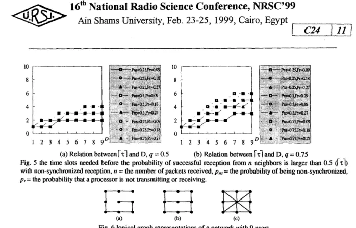
for dierent parameters

In Fig. 5(a)-(c),

we

evaluate another important parameter

rd

- number of time slots required in a stage of the broadcast algorithm. Following the convention in [14], we chose the same value P, =1/2 as the required value offlD,r) at the end of a stage. What differs from [14] is the number of required time slots in each stage, i.e.

hi.

It can be proved that 114,171 with the probability of successful reception in a stage (P,)=l/2, the number of time slots needed is within

hi

*

T(&) with probability larger than 1- E, where T(E) =2

*

R

+

5 M(E)*M~x(G .M(&)) and M(e) =

R(,log(N/&)) , where R is the radius of the network

For synchronized reception, from the results offln,r) such as that in Fig. 4(a), we can see that one time slot is enough forflat) to be larger than P f l . 5 . Therefore,for synchronized reception, r27= 1.

For non-synchronized reception, we investigate the influences of different p , and q. In Fig. 5 (a)-(b), the curves

hi

versus D for pN = 0.25,0.5,0.75, p , = 0.09,O. 18,0.27, and q = 0.5,0.75 are demonstrated. The case q = 0.25 was not considered because we found that P, = O S can not be reached for larger p m and p , with q = 0.25. We have the following findings from these numerical results in Fig. 5 (a)-(b),

Generally, the number of time slots needed

(z1)

such that f i D , rzl) 2 0.5 increases with D increasing. And the

relation is almost logarithmic asymptotically, i.e.,

r-d

grows with rate log(D), for non-synchronized reception. From Fig. 5(a)(b) and the fact that P, =OS can not be reached for larger pN andp, with q = 0.25, the best value of q

is around 0.5. If q is too small, it is possible that all processors stop transmitting too

soon.

If q is too large, the detrimental collisions will continue to occur for a longer period, andfin,r) will be increasing with t at a lower rate, as Fig. 4(b.3.1-3).

16“

National Radio

Science

Conference, NRSC’99

A h Shams

University,

Feb.

23-25,1999,

Cairo, Egypt

pil-q

The impact of pr is not serious

as

long as pr is within a reasonable range. Therefore, allowing the processors not to carry out broadcast temporarily does not damage the performance a lot. The processors can thus sometimes save power or deal with other urgent task. In fact, when the number of simultaneous transmitting neighbors is large, allowing the processors not to cany out broadcast might also be a method to solve collision of packets. For example,

as in Fig. 5(a,b), when pN

=

0.75,

rd

is smaller with larger p r (0.18,0.27) than with smaller p r (0.09).

Optimization of the network topology

The network topology can be decided by the transmission range 121 and the antenna direction (pattern) 1171. From

the above analysis, we can investigate the optimization problem mentioned in the beginning of this section.

From the result in [14] and Theorem 3, 4 in [17], the time needed to carry out broadcast for non-synchronized reception is proportional to

r d

*

i7&),

where

hi

grows almost logarithmically with D asymptotically, T(&) =2

*

R

+

5 M(&)*Max($ ,M(E)). Let N=!J and fk0.01, then 1og2(N/€)=9.8, M(&) =3.13.

Consider the three examples in Fig. 6: (a) D=2, R A ; (b) D=3, R=3; (c) D=8, R=2. We have Max($ .M(&))=3.13, and T(E) =2

*

R

+

5 *9.8 = 2Ri-49.

In the following, the value of

hi

is from Fig. 5(a). Consider the casep, = 0.5, p r = 0.18. (a) D = 2,

Tzl

=I; R=S, T(E) = 2*8+49=65; needs 1*65=65 time slots

(b) D=3,

r d

=2; R=3, T(&) = 2*3+49=55; needs 2*55= 110 time slots

(c) D=S, rzl=3; ~ = 2 , T(E) = 2*2+49=53; needs 3*53= 159 time slots

Therefore, for this case, the smaller the D, the less the time needed. R may be allowed to be larger. This is because the occurrence of collisions is the main obstacle of broadcast for non-synchronized reception.

For synchronized reception, the situation is in contrast to the situation for non-synchronized reception. Therefore, the smaller the R, the less the time needed. This is because the successful reception probability is better for larger D,

and the time needed by broadcast algorithm is in proportional to the radius (R).

V.

Conclusions

In this paper, we analyze the probability of successful reception of the packet when more than one packet are

received at the same time. The probability of successful reception is not only depending on the reception power of packets 1171, but also depending on the time lag and the contents of the collided packets. There is a great gap

between the performance of synchronized and non-synchronized reaeption. In broadcast, the performance of synchronized reception of several packets is in fact better than that of reception of only one packet. This is because the multiple packets received contain the same content, the symbols are synchronized, and the envelope magnitude of the sum of the signals is larger than that of only one signal. Besides, incoherent demodulation is used, so the envelope magnitude decides whether a packet

can

be received correctly. On the other hand, non-synchronized reception of the packets caused adverse effects. Since the symbols are not synchronized, the content of one packet acts as noise to other packets. Therefore, the receiving processor has a smaller chance to receive any one of the packets successfully. The substantial difference in performance of synchronized and non-synchronized reception also influences how the broadcast algorithm is used. For synchronized case, the processors in fact do not need to use “decay” to solve collision of packets, since collision of packets in fact enhances the probability of successful reception. For non- synchronized case, the processors need to use “decay” to solve collision of packets, since non-synchronized reception

of packets might

destroy

the packet. Therefore, the number of time slots needed in a stage is practically 1 for synchronized reception, and grows logarithmically with the maximum number of neighbors (i.e.,

lo@)

for non- synchronized reception.

We also investigate how to improve the performance. When collisions are not frequent and there are only few neighbors, raising q can keep the neighbors transmitting for longer time. When collisions are frequent, the time and power needed can be reduced by using smaller q to reduce the number of collisions. Raising the transmitter power and thus signal-to-noise ratio can only improve the performance within a limit, after which increasing power level does not result in great improvement. Rather, choosing a proper value of retransmission probability q is a more

effective way to improve performance.

How to optimize the network topology to reduce the time needed for broadcast also differs in the cases of synchronized and non-synchronized reception. Minimizing the time complexity requires minimizing both the radius

of the network R and the degree of the network 13. However, there is a tradeoff between

D

and R. For example, if the transmitters increase their power levels, R could decrease and D could increase, To reduce the time needed for broadcast, trying to have smaller R is a better method for synchronized reception, but trying to have smaller D is a

16th

National

Radio Science Conference,

NRSC’99

Ain

Shams University, Feb.

23-25,

1999,

Cairo,

Egypt

Practical processors might not carry out broadcast temporarily. In fact, for the case that collision is detrimental and collisions are firesuent, allowing the processors not to carry out broadcast temporarily might also be a method to solve collision of packets. We found that the performance degrades with p r (probability that a processor does not carry out broadcast) for synchronized reception, and the p e r f o m c e sometimes improves with pr for non- synchronized reception.

In multihop radio networks, broadcast provides an effective way to implement communications among users under the condition tha there is no base station. This is especially true for wireless local area networks, where synchronized reception can be more easily achieved. Furthermore, the mobility of users increases the cost of maintaining a routing table needed by deterministic algorithms. Therefore, randomized algorithms are more appealing. There are several directions €or future work First, the performance of multiple messages broadcast, routing, and multicast can be investigated [15,25]. Second, other possible methods of broadcast in multihop radio networks can also be studied. For example, how to carry out broadcast in a completely asynchronous (i.e. unslotted) manner can be studied. Third, we can carry out more accurate analysis of the probability of successful reception with practical considerations. One consideration is the correlation between consecutive events, such as severe fading, non-synchronized reception, and a processor’s pause in carrying out broadcast algorithm. Another consideration is the relation between successful reception at packet level and signaling level, Fourth, we will investigate possible performance improvements by the use of receiver diversity and RAKE receiver to distinguish and combine packets from different users [263.

References

[

11

D. P. Bertsekas and R. G. Gallager, Data Networks, Znd edition, Englewood Cliffs, NJ.: Prentice Hall,1992.

[2] D.

P. Bertsekas and J. N. Tsitsiklis, Parallel and Distributed Computation: Numerical M e l b d s , Englewood Cliffs, N.J. : Prentice Hall, 1989.

I31

U. Black, Mobile and Wireless Networks, Upper Saddle River, N. J. : Prentice Hall, 1996.

[4]

“802.1 1 Wireless LAN Medium Access Control

(MAC)

and Physical Layer (PHY) specifications,”

IEEE

Standards Board, June 1997.

[SI

T.-W. Chen, J.T. Tsai, and M. Gerla, “QoS routing performance in multihop, multimedia, wireless networks,” in Proc, ICVPC’97.

[61

C .4 . Chiang and M. Gerla, “Routing and multicast in multihop, mobile wireless networks,” in Proc. fCUPC’97.

[7]

C.-C. Chiang, H.-K. Wu, W. Liu, and M. Gerla, “Routing in Clustered Multihop Mobile Wireless Networks with Fading Channel,” in Proc. IEEE Singapore International Conference on Network (SlCON’97).

[SI

C. R. Lin and M. Gerla, “MACAPR: An Asynchronous Multimedia Multihop Wireless Network,” in Proc. INFOCOM ‘97.

191

I. CNamatic and 0. Weistein, “The Wave Expansion Approach to Broadcasting in Multihop Radio Networks,”

IEEE Transactions on Communications, vol. COM-39, No. 3, Mar. 1991, pp. 426433,

[lo]

M. Gerla and J. T. Tsai, “Multiculster, mobile, multimedia radio networks,” Wireless Networks, vol. 1, pp.

[11]

E. Pagani and G.P. Rossi, “Reliable broadcast in mobile multihop packet networks,” in Proc. MOBICOM’97, pp, 3442.

[

121

N. &on, A. Bar-Noy, N. Linial, and D. Peleg, “A Lower Bound for Radio Broadcast,” Journal of Computer andSystem Sciences, 43, 1991,290-298.

[

131

D. Bruschi and M. Del Pinto, “Lower bounds for the broadcast problem in mobile radio networks,’’ Distributed Computing, 1997 10, 129-135.

[14]

R. Bar-Yehuda, 0. Goldreich, and A. Itai, “On the Time-Complexity of Broadcast in Multi-hop Radio Networks: an Exponential Gap between Determinism and Randomization,” Journal of Computer and System Sciences, 45, 1992, 104-126.

[lS]

R. Bar-Yehuda, A. Israeli, and A. Itai, “Multiple communication in multi-hop radio networks,” SIAM J. Comput., 22, 1993, pp. 875-887.

[16]

E. Kushilevitz and Y. Mansour, “An rR(D log(N/D)) lower bound for broadcast in radio networks,” SIAM J. Comput., 27, 1998, pp. 702-712.

[17]

K.-H. Pan, H.-K. Wu, R-J. Shang, and F. Lai, “Performance analysis of distributed broadcast algorithms in

wireless networks with consideration of channel reliability,” accepted by PDCN98.

[18]

T. Tsiligirides, “Queueing analysis of a hybrid C S W C D and B T M A protocol with capture,“ Cornpurer Communications, 19 (1996), pp, 763 - 787.

16fh

National Radio Science Conference,

NRSC'99

Ain Shams University, Feb. 23-25, 1999,

Cairo,

Egypt

1-1

[

191

T . S. Rappaport, Wireless Communications: Principks and Practice, Prentice Hall PTR, New Jersey, 1996.

[20] R.

E. Ziemer and W. H. Tranter, Principles of Communications, Boston,

MA:

Houghton Mifflin: 1995, 4*

edition.

[21]

S . Haykin, Communication System, New York John Wiley & Sons, 1994, 3d edition.

[22]

R. M~twani and P. Raghavan, "Randomized Algorithms," Cambridge, New York, 1995.

[23]

J. W. Grossman, "Discrete Mathematics:

an

Introduction to Concepts, Methods, and Applications," Macmillan: NewYork, 1990.

[24]

R. L. Graham, D. E. Knuth, and 0. Patashnik, Concrete Mathematics, Addison-Wesley, 1991.

1251

G.D. Stamoulis and J N . Tsitsiklis, "Efficient Routing Schemes for Multiple Broadcasts in Hypercubes", IEEE Transactions on Parallel and Distributed Systems, Vol. 4, NO. 7, July 1993, pp. 725-739.

[26]

H.

V.

Poor and G. W. Womell (eds.), Wireless Communications: Signal Processing Perspectives, Upper Saddle River, NI: Prentice-Hall, 1998.

0.2

0 4

-0 0.1 0.2 0.3 0.4 0.5 0.6 0.7 0.8 0.9 1

T,: time lag between the arrivals of the packets (unit: symbol duration) take n = 2 in this case

Fig. 1 the relation between time lag and the probability that the packet is received successfully in a collision of n

(Prcceivcd )* 1.2 1 0.8 0.6 0.5 0.4 0.2 1.5 1 0 0 Pns 2 3 4 5 6 I 8 9 " 0 0.1 0.2 0.3 0.4 0.5 0.6 0.7 0.8 0.9

(a) Relation between Pmceivcd[nJ and n _{(b) Relation between} (Prccrivcd

tnl)

and pm.

Fig. 2 the probability that the packet is received successfully in a collision of n packets Prrccivc~nJ

1.2 I 0.9 0.8 0.1 0.6 0.6 0.5 0.4 0.3 0.4 0.2 - 0.2 0.1 O L I t ' ' ' i i 0 - - 0.03 0.06 0.09 0.12 0.15 0.18 0.21 0.M 0.2'7 Pr 1 2 3 4 5 6 7 8 9 '

(a. 1) Relation between Pm, a d p p

1 6th

National Radio Science Conference,

NRSC'99

Ain

Shams University, Feb. 23-25,1999,

Cairo, Egypt

0.9 0.8 0.7 0.6 0.5 0.4 0.3 0.2 0.1 0 1 0.9 0.8 0.7 0.6 0.5 0.4 0.3 0.2 0.1 0 4 - - - - - - - - - ' L U i L -1

r-

1 0.030.060.090.120.150.180.21 0.240.27 p r 1 2 3 4 5 6 1 8 9 n

(b. 1) Relation between PmcCeu and pr. (pm = 0.1) (b.2) Relation between Pswcess and n (pN = 0.2) (b) Non-synchronized reception

Fig. 3 the probability that the packet is received correctly from n neighbors PS-&], n = the number of packets received, Pr= the probability that a processor is not transmitting or receiving. Psmcsp the probability of successful receiving the packet from n neighbors

with

the packet. Pr: the probability that a processor is busy with other tasks.

1 0.9 0.8 0.7 0.6 0.5 0.4 0.3 0.2 0.1 0 L I I I I 1 2 3 4 5 6 1 8 g t (a.3) (b. 1 1 0.9 0.8 0.7 0.6 0.5 0.4 0.3 0.2 0.1 0 1 2 3 4 5 6 7 8 9 n

(a. 1) Relation betweenfin, t ) and 1. (a.2) Relation betweenfln, t) and n.

0.8

r---1

0.6 0.4 0.2

-!

0

pu,,_,i

1 2 3 4 5 6 7 8 9 t

2) Relation betweenfln, r) and I,

(b.l.1) R

q = 0.25, p N = 0.5

0.8 0.6

1 2 3 4 5 6 7 8 9

.elation betweenfln, r ) and t, q

0.6 0.4

0.2

) " " ' )

1 2 3 4 5 6 1 8 9 '

(b. 1.3) Relation between fin, r)

: 0.25, pw = 0.25

16th

National Radio Science Conference,

NRSC'99

Ain Shams University, Feb. 23-25, 1999,

Cairo,

Egypt

I

C24 110

1

1 0.8 0.6 0.4 0.2 0

cy-

1 2 3 4 5 6 1 8 9 t 1 0.8 0.6 0.4 0.2 0

7

1

1 2 3 4 5 6 7 8 9 f

(b.2.1) Relation betweenf(n,

r)

and r, q = 0.5, p,,, = 0.25 (b.2.2) Relation betweenfln, t ) and t, q = 0.5, pw = 0.5

(b.2

1 2 3 4 5 6 I

a

9 '

.3) Relation betweenfin, t ) and t, q = 0.5, p,,, = 0.75

1 0.8 0.6 0.4 0.2 0 (b.3. 1 2 3 4 5 6 1 8 9'

1) Relation betweenfln,r) and t , q = 0.75, pN = 3.25

1 2 3 4 5 6 7 8 9 ' _{1 2} 3 4 5 6 7 8 9 f

(b.3.2) Relation betweenfin, r ) and r, _{(b.3.3) Relation betweenfln, t ) and t, q = 0.75, pm = 0.75}

Fig. 4 the probability that the packet is received correctly from n neighbors in time r (fin, t ) ),n = the number of packet! received, p r = the probability that a processor is not transmitting or receiving. (a) Synchronized reception (b)

A

16fh

National Radio Science Conference,

NRSC'99

1-111)

WY

Ain Shams

University, Feb. 23-25, 1999, Cairo, Egypt

lo

I

1

i---i

(a) Relation between

hi

and D, q = 0.5 (b) Relation between

rd

and D, q = 0.75

Fig. 5 the time slots needed before the probability of successful reception from n neighbors is larger than 0.5

621)

with non-synchronized reception, n = the number of packets received, pN = the probability of being non-synchronized, p r = the probability that a processor is not transmitting or receiving.

(4 (b) (4