An alternative mean estimator for processes monitored by SPC charts

INT

.

J

.

PROD

.

RES

.,

2000, VOL

.

38, NO

.

13, 3093 ± 3109

An alternative mean estimator for processes monitored by SPC charts

ARGON CHENy* and E. A. ELSAYEDz

Statistical Process Control (SPC) chart is a graphical tool that helps to identify a possible process shift. Though the SPC chart is, in theory, a monitoring tool that reveals only the result of a statistical hypothesis testing, in practice the chart’s signaling is often used for making process adjustment. In this paper we develop a robust estimator of the process mean for processes monitored by SPC charts. This mean estimate can serve as an important reference for investigating assignable causes and taking appropriate corrective actions. When the control chart is imple-mented as a control device, the mean estimate can also provide a more accurate assessment of the amount of adjustment to be made to the process. We also demonstrate in this paper that when the process shift is relatively small, the proposed mean estimate outperforms the mean estimate usually used for the CUSUM scheme.

1. Introduction

SPC charts are very widely used in practice (Montgomery 1996). In particular, the Shewhart control chart (Shewhart 1931) developed more than 60 years ago remains the most popular, if not the most e€ ective, monitoring tool. Though the statistical theories and assumptions underlying the SPC chart have been fully dis-cussed, its employment draws continuous debates and discussions. Di€ erent types of industries have di€ erent needs in monitoring or controlling production processes. Therefore, distinct employment strategies are developed to accommodate the SPC charts. In some industries the chart is used as a straightforward monitoring device that warns workers of a possible out-of-control process. Other industries use it as a control device that alerts workers and provides a basis for process adjustment.

SPC charts are designed to detect shifts among natural ¯ uctuations caused by chance noises. For example, the Shewhart chart utilizes the standard deviation (SD) statistic to measure the size of the in-control process variability. By graphically contrasting the observed deviations against a multiple (usually, triple) of SDs, the control chart is intended to identify unusual departures of the process from its normal state (controlled state). Under certain assumptions, when the observed devi-ation from the mean exceeds three SDs, it is said that the process is out of control since there is only a probability of 0.0026 for the observation to fall outside the three SD limits given an unshifted mean chance the process mean is shifted. This Shewhart chart scheme is in e€ ect a statistical hypothesis testing that reveals only whether the process is still in-control. This is certainly not enough for practical applications

International Journal of Production Research ISSN 0020± 7543 print/ISSN 1366± 588X online#2000 Taylor & Francis Ltd http://www.tandf.co.uk/journals

Revision received February 2000.

{ Graduate Institute of Industrial Engineering, National Taiwan University, 1, Sec. 4, Roosevelt Rd., Taipei, Taiwan, 106.

{ Department of Industrial Engineering, Rutgers, The State University of New Jersey, 96 Frelinghuysen Rd., Piscataway, NJ 08854, USA.

where the causes of the problem should be found and removed to restore the pro-duction process to its satisfactory operational state.

It is the search for the out-of-control causes and the reinstatement of the process that complete the statistical process control loop. To reinstate the process, necessary corrective actions or process adjustment are performed following the chart’s signal-ing. Before corrective actions are taken, it is critical to search for the cause of the out-of-control occurrence. During this search process, a robust process mean esti-mate can serve as a valuable reference that helps to determine the size of the process deviation and thus limit the search to a selective set of possible causes. Sometimes, process adjustment is made following the out-of-control signal to bring the departed process back to the in-control state. The size of the adjustment is usually based on the runs pattern of the data points and most frequently on the judgment of experi-enced process engineers. An accurate estimate of the mean will certainly provide a more precise adjustment of the process. In this paper, a robust mean estimate for processes monitored by SPC charts is developed to ful® ll these needs.

In the literature, process mean estimates are usually developed for processes governed by a linear stochastic system and can be described using state-space models or autoregressive integrated moving average (ARIMA) models. Harrison and Stevens (1971, 1976), apply state-space models to situations where shifts are exhibited both in the process level and the slope. As the authors point out, their model for shifts in the mean is, in a way, analogous to the ARIMA (0, 1, 1) model in Box and Jenkins (1968, 1970). This integrated moving average (IMA or ARIMA (0, 1, 1)) model can be transformed into an exponentially weighted moving average (EWMA) estimator, which in turn can be realized as the popular PID controller. Recently, the EWMA estimator attracted the attention of both researchers (MacGregor 1988, Box and Kramer 1992, Ingolfsson and Sachs 1993, Yashchin 1995) and practitioners (Sachs et al. 1995, Boning et al. 1995).

Process adjustment based on process mean estimation is a feedback control scheme (AÊstroÈm 1970, Box and Jenkins 1968, 1970, Davis and Vinter 1985) that is generally referred to as the Automatic Process Control (APC) approach. Most of the researchers in the APC area focus on identifying the dynamic nature of the process and disturbance, and constructing a linear system to describe them. The SPC chart is intended to identify the process departure from its normal state. This is referred to as the SPC approach. Extensive discussions about APC and SPC can be found in MacGregor (1987, 1988), Box and Kramer (1992), Vander Wiel et al. (1992), Tucker et al. (1993) and Sachs et al. (1995). While we agree that these two approaches have their own roles and should not be obscured with their seemingly related names, we also think that a plausible mean estimate should be developed to provide a basis for further actions when a process is signaled out-of-control by a statistical control chart.

Barnard (1959) was the ® rst to point out the possibility of using control chart as an element in a feedback control loop. He suggests that the control chart should not only be used as a monitoring device but also as an estimator. The work, however, received limited attention from industrial practitioners. This is possibly because the cumulative sum (CUSUM) control chart (Page 1954, 1955, Cherno€ and Zacks 1964) used by Barnard is relatively complex and is less popular than the Shewhart control chart. The Shewhart chart remains the dominant control chart in practice because of its simplicity and the development of its supplementary runs rules (Hoerl and Palm 1992). Nevertheless, Barnard’s original idea provides a new perspective for

applications of control charts. Kelton et al. (1990) developed certain adjustment rules based on quality control charts but only looked on observations after the out-of-control point. Nishina (1992) investigated the problem of change-point estimation for control charts using accumulated data (CUSUM, EWMA and MA charts). In this paper we follow Barnard’s idea but focus on the popular Shewhart control chart ® rst. We then show how the approach can be applied to other types of control chart.

We start with the introduction in this section. The rest of this paper is organized into four sections. The process model is described and the basic assumptions behind SPC charts are discussed in the following section. In Section 3 we develop the mean estimate for the Shewhart chart with a single 3-s rule and a constant shift occurrence probability followed by an example and discussions. The mean estimate is then extended for Shewhart charts with supplementary runs rules and for SPC charts in general. An example will be given for the CUSUM scheme. Finally, we study a more realistic shift occurrence mechanism where the shift’s inter-occurrence time follows a renewal process. The idea is also illustrated using an example.

2. Process model

In this paper we will use the simple Shewhart control chart and a semiconductor fabrication process as examples to illustrate the SPC ideas and to demonstrate the use of the proposed mean estimate. One of the very important processes in semi-conductor manufacturing is to grow a layer of silicon dioxide (SiO2) by performing oxidation in a furnace. The critical output characteristic of the oxidation process is the thickness of the SiO2 layer. After oxidation, the thickness is measured in Angstrom (AÊ) and plotted on a Shewhart control chart to track the process condition. Very often, the process engineers use the control chart not only as a monitor of the furnace conditions but also a trigger for making adjustment to the furnace temperature.

Let the random variables X1;X2;X3;. . . denote the 1st, 2nd, 3rd, . . . successive sample statistics of the quality characteristic observations, say the thickness of the SiO2layer. The sample statistic Xican be a single observed value or a sample mean

of several observed values. It is assumed that Xiis normally distributed with mean ·i

and variance ¼2. In the Shewhart control scheme, the process mean · is initially set to coincide with the target (T ). For instance, let the target of the oxide thickness be 250 AÊ. When the process is in-control, Xi are said to have the same mean ·

…

ˆ 250

†

unless the following condition is violated:

·¡ 3¼ µ Xiµ ·

‡

3¼;

where · ¡ 3¼ and ·

‡

3¼ are the lower and upper control limits, respectively. Let the standard deviation (¼) of the thickness be 1.5 AÊ. When any of the control limits is exceeded, the process is said to be probably out-of-control; i.e. the process mean has probably departed from the target 250 AÊ. The chance for either one of the control limits to be exceeded at observation i given that the mean of Xiremains at 250 is

¬ˆ P

_…

Xi> 254:5j·i ˆ 250

†

‡

P

…

Xi< 245:5j·iˆ 250

†

ˆ

‰

1 ¡ F

…

3

_†

_{Š ‡}

F

_…

¡3

†

ˆ 2F

_…

¡3

†

ˆ 0:0026 ;

where F is the cumulative distribution function of a standard normal random variable. However, there is still a probability of 0.0026 that the observation falls

outside the control limits given an unchanged process mean. This probability is referred to as the probability of Type I error and is denoted by ¬.

When one of the control limits is exceeded at the ith observation, this does not mean that the process is out-of-control exactly at this sample point. The process could have been out-of-control long before i but the control limit was not exceeded until observation i. When the process is actually out-of-control but control limits are not exceeded, this misinterpretation of the process state is called Type II error. The probability of this Type II error’s occurrence can be calculated given the magnitude of the deviation in the mean. For instance, if the mean changes from 250 to 253 (that is, the mean of the thickness deviates from the target by 2¼), then the Type II error probability, denoted by ­ , using the Shewhart chart scheme is

­ ˆ P

_…

Xi 2

‰

245:5;254:5

Š

j·iˆ 253

†

ˆ F

…

3 ¡253 ¡ 250_1:5

†

¡ F

…

¡3 ¡253 ¡ 250_1:5

†

ˆ 0:841:

As mentioned earlier, this Shewhart scheme reveals only a hypothesis testing result. In the following sections, we will estimate the process mean when the Shewhart chart signals an out-of-control.

3. Basic estimation procedure for Shewhart chart

Before estimating the process mean based on the Shewhart chart’s signaling, we ® rst examine the case where the point of the mean change is known. Given this change point information, two conditional mean estimators can be easily derived. Suppose that the current observation is j and the most recent mean change occurred at observation k. A straightforward estimate of the process mean is the sample mean; i.e. the arithmetic average of observations k to j :

-x_jjk ˆ

Pj iˆkxi

j ¡ k

‡

1;

…

1

†

where xi is the observed value of Xi. Since the shift occurred at k, all observations

from observation k forward have the same mean. This justi® es (1). However, this estimate su€ ers from high instability especially when the sample size j ¡ k

‡

1 is small. After enough experience has been accumulated and information about the amount of mean changes has been gathered, the past experience can actually serve as the prior knowledge on how the process mean is likely to shift. Baye’s estimation technique can then be applied to stabilize the mean estimate. Since the SPC chart’s assumption about the process is normal distribution, a proper conjugate prior distri-bution is, therefore, also a normal distridistri-bution. Let the prior distridistri-bution’s mean be ¹ and variance be ½2. Bayes estimator under a quadratic loss function can be obtained (Lehmann 1991, pp 236± 249) as follows:

^

·_jjk ˆ ½2x-_jjk

_‡

¼ 2 j ¡ k

‡

1¹ ¼2 j ¡ k

‡

1

‡

½ 2 :

_…

2

_†

By examination of (2), one can ® nd that when the number of observations ( j ¡ k

‡

1) between the current point and the change point is large, then more weight is assigned to -xjjk. On the other hand, when j ¡ k

‡

1 is small, ¹ is assigned

a higher weight; that is, the past experience becomes more important in the estimate. Also, the mean estimate approaches ¹ when ½2 is relatively small. This is because a small ½2 means that we learn from experience that the process mean moves to a deterministic value ¹ whenever a shift occurs. In addition, the Bayes estimator has been elegantly crafted to prevent the estimator from diverging for the case of a large ½2since the larger the ½2the less the weight assigned to the prior knowledge on the shift size (¹). In fact, when ½2 is large, which means a very unreliable prior knowl-edge, one should really use the estimator in (1) instead of the Bayes estimator in (2). We have estimated the process mean given that the change point is known. The change point is, however, unlikely to be known. The Shewhart chart is thus devised to detect the process change. The control chart does not reveal the actual location of the change point either. In other words, with the control chart detection we only know that a mean change may have occurred at or before this detection point. To more accurately estimate the process mean we need to know where the change point is likely to reside. A lag-window of observation points prior to the control chart’s detection is de® ned to include all possible points at which the shift might occur.

Suppose that the current control chart’s detection point is at S2 and the one preceding it is at S1. In practice, corrective actions are taken after S1, and when the process is in operation again the process mean is immediately subject to possible new shifts. As shown in ® gure 1, the lag-window is de® ned as the time period containing all observation points between S1and S2 including S2. The lag-window’s de® nition depends greatly on the out-of-control practice. In any case, the lag-window’s starting point should lie at the point where the process is deemed back to its mean condition.

Given the current detection point at S2, it is plausible to say that a shift has occurred in the lag-window. Let the random variable K represent the exact location at which the shift occurs. We would like to know the probability distribution of K:

P_kjS2ˆ Pr

_…

K ˆ kjdetection at S2;K2

…

S1;S2

Š

†

:

It should be noted that when the control chart gives an alarm and the process mean needs to be re-estimated it is assumed that one and only one process shift indeed occurs in the lag-window. That is, it is assumed that with preliminary investigation of the alarm, the false alarm possibility has been ® rst ruled out. This assumption, however, is not unrealistic since in most cases alarms will be investigated and the shifted mean is only estimated for the out-of-control occurrence. There also exists a slim probability for more than one process shift to occur in the lag-window. The only

Lag-Window S1 S1+1 k S2 j previous detection point current detection current observation

one assumed shift occurrence actually accounts for the very last shift that determines the latest process condition.

Applying Bayes’ theorem, the probability that a shift occurs at a speci® c obser-vation point, say k, in the lag-window given the control chart detection at S2can be expressed as: P_kjS2 ˆP

…

K ˆ k; detection at S2jK 2

…

S1;S2

Š

†

P

_…

detection at S2jK 2

…

S1;S2

Š

†

ˆ P

…

detection at S2jK ˆ k;K 2

…

S1;S2

Š

†

P

…

K ˆ kjK 2

…

S1;S2

Š

†

PS2 lˆS1‡1 P

_…

detection at S2jK ˆ l;K 2

…

S1;S2

Š

†

P

…

K ˆ ljK 2

…

S1;S2

Š

†

:

…

3

†

To compute P_kjS2, two probabilities P

_…

detection at S2jK ˆ k;K 2

…

S1;S2

Š

†

and

P

_…

K ˆ kjK 2

_…

S1;S2

Š

†

need to be calculated.

P

_…

detection at S2jK ˆ k;K 2

…

S1;S2

Š

†

is the probability for the shift to be dis-covered at S2 given that the shift is known to occur at k; that is, K ˆ k and

K 2

_…

S1; S2

Š

. This probability can be seen as the probability of taking S2¡ k

‡

1 observations to detect the mean change. S2¡ k

‡

1 is also called the run length, i.e. the number of observations elapsed since the change point, before the control chart signals. Given an estimate of the shift size, one can calculate Type II error prob-ability (­S₂jk), and the run length probability distribution is simply the geometric distribution with the parameter ­S2jk:

P

_…

detection at S2jK ˆ k;K 2

…

S1;S2

Š

†

ˆ ­_SS₂2_jk¡k

…

1 ¡ ­S₂jk

†

:

…

4

†

Equation (4) can be explained as follows. When the mean is shifted at k, the shift is not detected (with Type II error probability ­S2jk) until observation S2 (with

prob-ability 1 ¡ ­S2jk). To calculate ­S2jk, one should know ® rst how much the mean is

shifted. Since the shift occurred at k, the shifted mean can be estimated by (1) or (2).

^

­S₂jk ˆ F 3 ¡

^

·S2jk¡ T ¼

…

†

¡ F ¡3 ¡·

^

S2jk¡ T ¼

…

†

:

…

5

†

P

_…

K ˆ kjK 2

…

S1;S2

Š

†

is the probability that the shift occurs at k given that the shift is known to be in the lag-window. To calculate this probability, we need to consider the probability for a shift to occur at any time. Here, we ® rst assume that the occurrence probability at any given time is constant p. Under this assumption, we can obtain : P

_…

k ˆ kjK 2

…

S1;S2

Š

†

ˆ p

…

1 ¡ p

†

S2¡S1¡1 S2¡ S1 1 p

…

1 ¡ p

†

S₂¡S1¡1 ˆ 1 S2¡ S1:

…

6

†

Substituting (4) and (6) into (3), we have P_kjS2ˆ ­

^

S2¡k S2jk

…

1 ¡­

^

S2jk

†

PS₂ lˆS1‡1

^

­S2¡l S₂jl

…

1 ¡­

^

S2jl

†

:

_…

7

_†

^

·S₂ ˆ XS2 KˆS1‡1

^

·S₂jKPKjS2;

…

8

†

where·

^

S2jKis the estimated mean of XS2given a known change point at K and PKjS2

is the probability for the shift to occur at K given a control chart detection at S2. When the process is not shut down after the control chart’s signaling and observation samples taken from the process are continued, then the process mean can be estimated for later observation points, say j and j > S2, in the same manner:

^

·j ˆ XS2 KˆS1‡1

^

·_jjKP_KjS2;

…

9

†

where P_KjS2 ˆ ­

^

S₂¡K jjK

…

1 ¡­

^

jjK

†

PS2 lˆS1‡1

^

­S2¡l jjl

…

1 ¡­

^

jjl

†

…

10

_†

and

^

­_jjKˆ F 3 ¡·

^

jjK¡ T ¼

…

†

¡ F ¡3 ¡·

^

jjK¡ T ¼

…

†

:

As mentioned earlier, the mean estimate given in (9) is in essence a weighted average of the observations. When·

^

_jjKis estimated by X-_jjK, we can summarize the weights for each observation Xi as follows:

^

·j ˆ X S₂¡1 iˆS1‡1 Xi KˆS1‡1 P_KjS2 j ¡ K

‡

1Xi

‡

Xj iˆS2 XS2 KˆS1‡1 P_KjS2 j ¡ K

‡

1Xi:

…

11

†

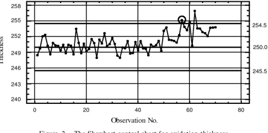
As an example, in the oxidation process the target SiO2 thickness is 250 AÊ. After preventive maintenance (PM), the process is in operation with process mean set to the target. Also, the thickness SD is known to be 1.5 AÊ. A Shewhart control chart is then constructed to monitor the oxidation condition. We have 70 observations. The thickness mean is shifted at the 50th observation with a magnitude 3.0 AÊ to become 253 AÊ. Figure 2 shows the corresponding Shewhart control chart. In the ® gure we assume that the true mean is known before the 50th observation.

As can be seen, at observation 57 the control chart gives an alarm. We now apply the mean estimate to this detection observation and the observations that follow. The lag-window includes observations 1 to 57. That is, the shift could have actually occurred at any of these observations. To compute the mean estimate for the detec-tion observadetec-tion 57, we ® rst calculate sample means for -x_57j57; -x_57j56;. . . ; -x_57j1. Corresponding to these sample means, we can estimate Type II error probabilities ­_57j57; ­_57j56; . . . ;­_57j1using (5):

­_57jKˆ F

…

3 ¡·

^

57jK_1:5¡ 250

†

¡ F

…

¡3 ¡·

^

57jK_1:5¡ 250

†

for K ˆ 1;. . . ;57: The shift occurrence probability given signaling at 57 can then be estimated using (7):

P_Kj57ˆ ­ 57¡k 57jK

…

1 ¡ ­57jK

†

P57 lˆ1­ 57¡l 57jl

…

1 ¡ ­57jl

†

for K ˆ 1;. . . ;57: The mean estimate for observation 57 is calculated as

^

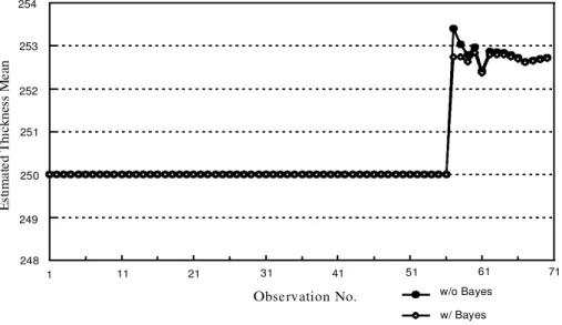
·57ˆ X57 Kˆ1 -x_57jKP_Kj57:

The same procedure is repeated for estimating means for observations 58 and beyond. Figure 3 shows the estimated mean together with the observations.

One can observe from ® gure 3 that the mean estimate at the signal observation overshoots a little given only one observation available after detection. The mean

0 20 40 60 80 240 243 246 249 252 255 258 T hi ck ne ss 250.0 254.5 245.5 Observation No.

Figure 2. The Shewhart control chart for oxidation thickness.

242 244 246 248 250 252 254 256 Observation No. T hi ck ne ss observations mean estimate 1 11 21 31 41 51 61 71 25

estimate is also seen to oscillate before it gradually stabilizes. Using the Bayes estimate given by (2), when enough experience has been gained, can signi® cantly reduce the overshooting and the oscillation at the beginning of the estimation. Suppose that the shifted mean has learned to vary around 252.5 AÊ with S.D. 2.0 AÊ. Then

^

·_jjKˆ 4:0 -x_jjK

‡

2:25 j ¡ k

‡

1252:5 2:25 j ¡ k

‡

1

‡

4:0 ; for K ˆ 1;. . . ;57:

Figure 4 shows a comparison between mean estimates with and without the Bayes stabilization.

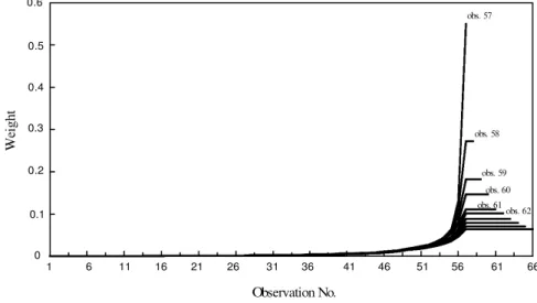
The Shewhart-based mean estimate is a weighted average of available observa-tions. It is interesting to see how the weights vary over the age of the observation. Figure 5 shows the weights assigned by the estimator to the past observations.

From Figure 5, the proposed mean estimate looks very much like a dynamic weighted average of available observations. For example, for the detection observa-tion’s mean estimate, the weight taken on observation 57 itself is about 0.55 and then decreases exponentially for older observations. When the mean estimate continues for observations after signaling, the weight distribution is dynamically adjusted. While the weights exponentially decrease for those observations sampled before detection, the observations after signaling are equally weighted. Take observation 62 as an example, the mean estimate for this data point takes observations 57 to 61 with an equal weight about 0.1. However, weights for observations 56 and earlier decrease drastically. This kind of weight distribution seems quite plausible for the situation where the out-of-control occurrence takes only the form of mean shift and its occurrence is solely tested by the Shewhart chart.

248 249 250 251 252 Observation No. E st im at ed T hi ck ne ss M ea n 254 253 1 11 21 31 41 51 61 71 w/o Bayes w/ Bayes

4. Mean estimate for other SPC charts and Shewhart chart with runs rules

It is well known that the original Shewhart chart is not e€ ective in detecting smaller process shifts. The popularity of the Shewhart chart lies not only on its simplicity but also on the development of customized runs rules. In addition to improving the control chart’s ability in detecting shifts, runs rules (Statistical Quality Control Handbook 1956) can be installed to identify patterns that are rather di cult to detect by the single out-of-3¼ rule.

The e€ ectiveness of a Shewhart chart is usually evaluated by Type I and Type II error probabilities. When runs rules are applied to Shewhart charts or other types of SPC charts, such as EWMA or CUSUM charts (Montgomery 1996), are used, the testing is not only based on a single observation but also on past observations. Here, run lengths (RLs) are used instead to evaluate the control chart’s ability. While the in-control RL (RL0) assesses how frequently the control chart gives false alarms, the out-of-control RL (RL1) measures how quickly the control chart signals a process shift. To evaluate the RLs, one can apply the Markov chain approach to ® nd its probability distribution (Brook and Evans 1972, Champ and Woodall 1987, and Lucas and Saccucci 1990).

As explained in the previous section, the out-of-control run length (RL1) prob-ability given an approximated shift size is needed in order to calculate P_kjS2. That is, we need to calculate

PS2jk ˆ P

…

detection at S2jK ˆ k;K 2

…

S1;S2

Š

†

ˆ P

_…

RL1ˆ S2¡ k

‡

1jshift ˆ·

^

jjk¡ T

†

…

12

†

for j

_¶

S2.

Depending on the runs rules or types of control charts used, the calculation of the run length probability can become extensive. For example, it takes 216 states in the Markov chain to calculate the run length distribution when the four runs rules listed above are implemented simultaneously. As for EWMA and CUSUM charts, the larger the number of states, the more accurate the RL distribution. For on-line

0 Observation No. W ei gh t obs. 57 obs. 58 obs. 59 obs. 62 obs. 61 obs. 60 0.6 0.5 0.4 0.3 0.2 0.1 1 6 11 16 21 26 31 36 41 46 51 56 61 66

production use, computer programs will be required for the calculation of RL dis-tributions and mean estimate. For the calculation procedure using the Markov chain approach, please refer to the references given above.

Because of the complexity of RL distribution calculations, we propose an approximation based on the simple geometric distribution. That is

­_jjk º 1 ¡_ARL1 1 and PS2jk ˆ P

…

RL1ˆ S2¡ k

‡

1jshift ˆ·

^

jjk¡ T

†

ˆ 1 ¡ 1 ARL1

…

†

S2¡k ₁ ARL1; j

¶

S2;

…

13

_†

where ARL1ˆ E

…

RL1ˆ S2¡ k

‡

1jshift ˆ·

^

jjk¡ T

†

. Since the calculations of

aver-age RLs (ARLs) are much simpler, usually by using an integral equation (Crowder 1989, Fellner 1990), than computing the entire distribution probabilities, this approximation will allow us to easily implement the proposed mean estimate.

The CUSUM chart is known for its superior ability in detecting small process shifts. The tabular CUSUM statistics are computed as follows:

C‡

i ˆ max

‰

0;xi¡

…

·0

‡

k¼

†

‡

C‡_i¡1

Š

C¡

i ˆ max

‰

0;xi¡

…

·0

‡

k¼

†

‡

Ci¡1¡

Š

;

where the starting values C‡

0 ˆ C0¡ˆ 0. If either C‡i or C¡i exceeds h¼, the process is

considered out of control. To retain ARL0 around 370 and a relatively good per-formance of ARL1;k and h are usually set equal to 1/2 and 4.5, respectively. The ARLs of this CUSUM scheme for di€ erent shift sizes can be easily approximated by the following formula (Siegmund 1985) :

ARL º exp

_…

_¡2

D

b

_†

‡

2

D

b ¡ 1 2

D

2 for

D

6ˆ 0 b2 for

D

ˆ 0; 8 < :

where

D

ˆ ¯ ¡ k for the upper one-sided CUSUM, b ˆ h

‡

1:166, and ¯ˆ

_…

expected shift ¡ ·0

†

=¼. To test our mean estimate approach for CUSUM charts, we use Siegmund’s ARL formula and the geometric distribution approxima-tion for the calculaapproxima-tions of run length probabilities. We shall also compare our approach to a mean estimator (Montgomery 1996) usually used for the tabular CUSUM chart:

^

·ˆ ·0

‡

k¼

‡

C ‡ i N‡ if C‡i > H ·0

‡

k¼

‡

C ¡ i N¡ if Ci¡> H ; 8

>

>

>

_<

>

>

>

_:

where N‡_{and N}¡_{represent the number of consecutive periods that C}‡

i or Ci¡have

been nonzero.

The performance of the mean estimators is measured by mean squared deviation (MSD) of 50 mean estimates from the true mean after the ® rst alarm of the CUSUM

chart. This mean squared deviation is then normalized against the process standard deviation ¼:  MSD50 p ¼ ˆ  P S₂‡49 iˆS2

…

·i¡·

^

i

†

2 50¼2 v u u u t :

Only ® fty observations after the out-of-control signal are taken to calculate the mean squared deviation because corrective actions are likely to be taken within these runs and the mean estimators become relatively steady after 50 observations. Also, since the CUSUM chart’s design is usually aimed for smaller process shifts. We compare the performance of mean estimators for shift sizes: 0.25¼, 0.5¼, 0.75¼, 1¼, 1.25¼ and 1.5¼. Results, shown in ® gure 6, are based on 2000 simulation runs with standard errors less than 0.5%.

It can be seen from ® gure 6 that our mean estimator outperforms the CUSUM mean estimator for process shifts less than 1.25¼. The estimator, however, su€ ers from unstable approximations of ARL and RL probability distribution and becomes less accurate for mean shifts greater than 1.25¼. Since the CUSUM scheme is espe-cially designed to detect smaller process shifts, the usual CUSUM mean estimator apparently lacks the estimation power for such shifts and our proposed estimator should be used instead. It can be also observed from ® gure 6 that our mean estimator is more robust than the CUSUM mean estimator especially for mean shifts less than 0.5¼.

5. Mean estimate for general shift occurrence mechanism

We assume in the basic estimation procedure that the probability for a shift occurrence at any observation is constant p. We now consider a more realistic case where the probability of the shift occurrence is not constant and the shift inter-occurrence time follows a general continuous distribution with pdf f

_…

t

_†

. We

Observation No. E st im at ed T hi ck ne ss M ea constant p Weibull(2, 300) 254 253 252 251 250 249 248 1 11 21 31 41 51 61 71

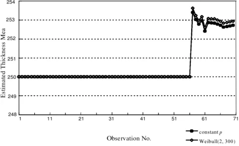
Figure 6. Mean estimates for constant shift occurrence probability and Weibull distributed inter-occurrence time.

assume that the shift occurrence is a renewal process; that is, the time duration between consecutive shifts is positive, independent, identically distributed with pdf f

_…

t

_†

. Because of the availability of a large number of continuous distributions, the continuous time renewal process will allow us to model a wide range of shift occur-rence mechanisms.

Under the above assumptions, the starting point of the inter-occurrence renewal cycle actually coincides with the starting point of the lag-window de® ned earlier; that is, the cycle starts at S1

‡

1. Then

P_kj…S₁;S₂Šˆ P

…

K ˆ kjK 2

…

S1;S2

Š

†

ˆP

…

a shift occurs in

…

k ¡ 1;k

Š

; say t; and no shifts in

…

t;S2

Š

†

P

_…

N

_…

hS2¡ hS1

†

ˆ 1

†

where h is the time interval between two consecutive observations and N

_…

hS2¡ hS1

†

ˆ 1 implies that the number of shifts in the interval

…

S1;S2

Š

is one. Further results can be carried out as follows (Cox 1962):

P

_…

N

_…

hS2¡ hS1

†

ˆ 1

†

ˆ P

…

N

…

hS2¡ hS1

¶

1

†

¡ P

…

N

…

hS2¡ hS1

†

¶

2

†

ˆ F

_…

hS2¡ hS1

†

¡ F2

…

hS2¡ hS1

†

ˆ …hS2¡hS1 0

‰

1 ¡ F

…

hS2¡ hS1¡ t

†

Š

f

…

t

†

dt where F

_…

T

_†

ˆ …T 0 f

…

t

†

dt ˆ P

…

N

…

T

†

¶

1

†

and F2

…

T

†

ˆ …T 0 F

…

T ¡ t

†

f

…

t

†

dt ˆ P

…

N

…

T

†

¶

2

†

Similarly, the probability that a shift occurs in

_…

_{k ¡ 1;k}

_Š

, say at t, and no other shifts occur in

_…

t;S2

Š

can be calculated as:

…h_…k¡S1† h_…k¡S1¡1† P

_…

N

_…

hS2¡ hS1¡ t

†

ˆ 0

†

f

…

t

†

ˆ …h_…k¡S1† h_…k¡S1¡1†

‰

1 ¡ F

…

hS2¡ hS1¡ t

†

Š

f

…

t

†

dt: Thus P_kj…S1;S2Šˆ …h_…k¡S1† h_…k¡S1¡1†

‰

1 ¡ F

…

hS2¡ hS1¡ t

†

Š

f

…

t

†

dt …hS2¡hS1 0

‰

1 ¡ F

…

hS2¡ hS1¡ t

†

Š

f

…

t

†

dt :

…

14

†

When the inter-occurrence time is exponentially distributed with parameter ¶, then P_kj…S₁;S2Šˆ „h_…k¡S1† h_…k¡S1¡1†e ¡¶…hS2¡hS1¡t†_¶e¡¶t_dt ¶

…

S2¡ S1

†

he¡¶…S2¡S1†h ˆ 1 S2¡ S1:

This is the same result as that of (6). In fact, the constant probability of shift occurrence model results in a geometric distribution of the shift inter-occurrence time which is a discrete `version’ of the exponential distribution. Both of them share the `memoryless property’.

Now, we consider a more general case by substituting (12) and (14) into (3) to obtain

P_kjS2 ˆ PS2jkPkj…S1;S2Š

PS₂ lˆS1‡1

PS₂jlPlj…S₁;S₂Š

:

_…

15

_†

Finally, (9) can be rewritten for general cases where runs rules are used and the shift occurrence follows a renewal process:

^

·jˆ XS2 KˆS1‡1

^

·_jjK PS2jKPKj…S1;S2Š PS2 lˆS1‡1 PS2jlPlj…S1;S2Š ;

…

16

†

where·

^

jjKis from (1) or (2) and PS₂jKand PKj…S₁;S2Šare from (12) (or (13)) and (14),

respectively.

Back to the semiconductor manufacturing problem: when an adjustment mechanism is present, the objective would be to adjust the process such that the mean of the thickness is as close as possible to the target. In the oxidation process, the furnace temperature is usually used as the adjustment variable. Given the estimate of the shifted mean in (16), the process engineer can now adjust the temperature to compensate for the thickness deviation·

^

j¡ T .

Continuing the earlier example, suppose that the process engineer has collected information on the frequency of Shewhart chart signals, other than false alarms. The time interval between two successive signals can be properly treated and modeled to serve the modeling of shift inter-occurrence time. Weibull distribution is often used for modeling `time to failure’ of a piece of device or equipment and is also appro-priate for modeling `time to shift’ of a process. The pdf of the Weibull distribution is:

f

_…

t

_†

ˆ ¬­ ¡¬t

¬¡1_e¡…t=­†¬

if t > 0

0 otherwise

(

where ¬ is the shape parameter and ­ is the scale parameter. For the oxidation process, suppose that ¬ and ­ are estimated to be 2 and 300, respectively; i.e., the mean time to shift is about 266 hours. The speci® c chemical process required to deposit a layer of 250 AÊ of SiO2takes about 2.5 hours to complete; that is, thickness samples are taken every 2.5 hours (h ˆ 2:5). Using (14), we obtain:

P_kj…0;57Šˆ …2:5k 2:5…k¡1†

…

2

_†…

300

_†

¡2_{t exp ¡} 142:5 ¡ t 300

…

†

2¡

…

₃₀₀t

†

2 " # …142:5 0

…

2

†…

300

†

¡2_{t exp ¡} 142:5 ¡ t 300

…

†

2¡

…

₃₀₀t

†

2 " # :

P_kj…0;57Š, together with the previously calculated P57jk using ­57jk is substituted into (15), we obtain new mean estimates as shown in ® gure 7. Again, we assume that the true mean is known before the 50th observation.

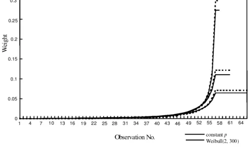
In ® gure 7 the newly estimated means are contrasted to the mean estimates assuming constant shift occurrence probabilities. As can be seen, the estimated mean also overshoots at the beginning of the process but stabilizes closer to 253 AÊ. This is because the weights assigned to the more recent data have shifted upward as shown in ® gure 8.

Unlike the constant occurrence probability, the occurrence probability for the Weibull model increases as time elapses. That is, more recent data are assigned more weights as described in (11) and (15) and demonstrated in ® gure 8.

Finally, the Bayes estimate can be used again to reduce the overshooting and ¯ uctuation at the beginning of the estimation.

Observation No. W ei gh t constant p Weibull(2, 300) 0.3 0.25 0.2 0.15 0.1 0.05 0 1 4 7 10 13 16 19 22 25 28 31 34 37 40 43 46 49 52 55 58 61 64

Figure 7. Weights taken by mean estimates for constant shift occurrence probability and Weibull distributed inter-occurrence time.

Observation No. T h ic k ne ss Observations Weibull w/o Bayes Weibull w/ Bayes 258 256 254 252 250 248 246 244 242 1 11 21 31 41 51 61 71

Figure 8. Mean estimates for Weibull distributed inter-occurrence time with Bayes stabilization.

6. Conclusions

In this paper we have developed methodologies to estimate the process mean for processes monitored by SPC charts to test possible process shifts. The proposed mean estimate was actually a dynamically weighted average of the historical data. It estimated the SPC chart’s test sensitivity and dynamically adjusted the weights of the historical data. The mean estimate was further re® ned by utilizing prior knowl-edge on the shift occurrence rate and shift size. The use of the mean estimate was then demonstrated through an example of the semiconductor oxidation process. The performance of the proposed mean estimator was shown to outperform a CUSUM mean estimator for shift sizes less than 1.25¼.

References

ÅSTRO

ï

M

,

K

.

J

.,

1970, Stochastic Control T heory (New York: Academic Press).

BARNARD

,

G

.

A

.,

1959, Control charts and stochastic processes. Journal of the Royal Statistics

Society, Series B, 21, 239± 257.

BONING

,

D

.,

HURWITZ

,

A

.,

MOYNE

,

J

.,

MOYNE

,

W

.,

SMITH

,

T

.,

TAYLOR

,

J

.

and TELFEYAN

,

R

.,

1995, Run by run control of chemical mechanical polishing. IEEE T ransactions

on Components, Packaging and Manufacturing T echnology Ð Part C, 19, 307± 314.

BOX

,

G

.

E

.

and JENKINS

,

G

.

M

.,

1968, Some recent advances in forecasting and control.

Applied Statistics, 17, 91± 109 ; 1970, T ime Series Analysis: Forecasting and Control

(San Francisco: Holden-Day).

BOX

,

G

.

E

.

andKRAMER

,

T

.,1992, Statistical process monitoring and feedback adjustment ± a

discussion. T echnometrics, 34, 251± 285.

BROOK

,

D

.

andEVANS

,

D

.

A

.,

1972, An approach to the probability distribution of CUSUM run length. Biometrika, 59, 539± 549.

CHAMP andWOODALL

,

1987, Exact results for Shewhart control charts with supplementary runs rules. T echnometrics, 29, 393± 399.

CHERNOFF

,

H

.

and ZACKS

,

S

.,

1964, Estimating the current mean of a normal distribution which is subject to change in time. Annals of Mathematics and Statistics, 35, 999± 1018. COX

,

D

.

R

.,

1962, Renewal T heory (New York: Chapman and Hall).

CROWDER

,

S

.

V

.,

1989, Design of exponentially weighted moving average schemes, 21, 155± 162.

DAVIS

,

M

.

H

.

A

.

andVINTER

,

R

.

B

.,

1985, Stochastic Modeling and Control (New York: Chapman & Hall).

FELLNER

,

W

.

H

.,

1990, Algorithm AS 258. Average run length for cumulative sum schemes.

Applied Statistics, 39, 402± 412.

HARRISON

,

P

.

J

.

and STEVENS

,

C

.

F

.,

1971, A Bayesian approach to short-term forecasting.

Operational Research Quarterly, 22, 341± 362; 1976, Bayesian forecasting. Journal of Royal Statistics Society, Series B, 38, 205± 247.

HOERL

,

R

.

W

.

andPALM

,

A

.,1992, Discussion: integrating SPC and APC. T echnometrics, 34,

268± 272.

INGOLFSSON

,

A

.

and SACHS

,

E

.,

1993, Stability and sensitivity of an EWMA controller.

Journal of Quality T echnology, 25, 271± 287.

KELTON

,

W

.

D

.,

WALTON

,

M

.,

HANCOCK

,

M

.

and BISCHAK

,

D

.

P

.,

1990, Adjustment rules based on quality control charts.International Journal of Production Research, 28, 385± 400.

LEHMANN

,

E

.

L

.,

1991, T heory of Point Estimation (Paci® c Grove, California: Wadsworth), pp. 236± 249.

LUCAS

,

J

.

M

.

and SACCUCI

,

M

.

S

.,

1990, Exponentially weighted moving average control schemes: properties and enhancements. T echnometrics, 32, 1± 27.

MACGREGOR

,

J

.

F

.,

1987, Interfaces between process control and online statistical process control. Computing and Systems T echnology Division Communications, 10, 9± 20; 1988, On line statistical process control. Chemical Engineering Progress, Oct., 21± 31. MONTGOMERY

,

D

.

C

.,

1996, Introduction to Statistical Quality Control (New York: Wiley). PAGE

,

E

.

S

.,

1954, Continuous inspection schemes. Biometrika, 41, 100± 116 ; 1955, A test for a

SACHS

,

E

.,

HU

,

A

.

andINGOLFSSON

,

A

.,1995, Run by run process control: combining spc and

feedback control.IEEE T ransactions on Semiconductor Manufacturing, 8, 26± 43. SIEGMUND

,

D

.,1985, Sequential Analysis: T ests and Con® dence Intervals (New York:

Springer-Verlag).

SHEWHART

,

W

.

A

.,1931, Economic Control of Quality Improvement (Princeton: Van Nostrand

Reinhold).

NISHINA

,

K

.,

1992, A comparison of contro charts from the viewpoint of change-point esti-mation. Quality and Reliability Engineering International, 8, 537± 541.

TUCKER

,

W

.

T

.,

FALTIN

,

F

.

W

.

andVANDERWIEL

,

S

.

A

.,

1993, Algorithmic statistical process control: an elaboration. T echnometrics, 35, 363± 375.

VANDER WIEL

,

S

.

A

.,

TUCKER

,

W

.

T

.,

FALTIN

,

F

.

W

.

and DOGANAKSOY

,

N

.,

1992, Algorithmic statistical process control: concepts and an application. T echnometrics, 34, 286± 297.

Western Electric Company, 1958, Statistical Quality Control Handbook (New York: Western Electric Company).

WOODALL

,

W

.

H

.

andREYNOLDS

,

M

.

R

.

R

.,Jr., 1983, A discrete Markov chain representation

of the sequential probability ratio test. Communications in Statistics Ð Sequential Analysis, 2, 27± 44.

YASHCHIN

,

E

.,

1995, Estimating the current mean of a process subject to abrupt changes.