大規模分散式L1正則化線性分類問題的有限記憶體共同方向最佳化演算法

全文

(1)國立臺灣大學電機資訊學院資訊工程學系學士班學生論文 Department of Computer Science and Information Engineering College of Electrical Engineering and Computer Science. National Taiwan University Bachelor Degree Thesis. 大規模分散式 L1 正則化線性分類問題的有限記憶體共同方向最佳化演算法 Limited-memory Common-directions Method for Distributed L1-regularized Linear Classification. 李鈺昇 Yu-Sheng Li. 指導教授：林智仁博士 Advisor: Chih-Jen Lin, Ph.D.. 中華民國 107 年 4 月 April, 2018.

(2)

(3) 摘要以分散式線性分類而言，L1 正則化非常有用，因為通常可以產生較小的模型。不過由於其不可微分性，開發高效的最佳化演算法十分困難。在過去十幾年，OWLQN 成為分散式 L1 問題最主流的解法。本文指出一些 OWLQN 的搜尋方向的問題，並將最近被開發出的用於 L2 問題的有限記憶體共同方向演算法延伸到 L1 問題。我們針對用於 L1 問題的批量方法給出一個統整性的解釋，並說明為什麼 OWLQN 是這麼流行的解法、以及為什麼我們提出的方法在分散式的環境下更高效。實驗也佐證我們的方法在多數情況下都比 OWLQN 更快速。關鍵字：大規模線性分類、牛頓法、分散式訓練、L1 正則化. ii.

(4) Abstract For distributed linear classification, L1 regularization is useful because of a smaller model size. However, with the non-differentiability, it is more difficult to develop efficient optimization algorithms. In the past decade, OWLQN has emerged as the major method for distributed training of L1 problems. In this work, we point out issues in OWLQN’s search directions. Then we extend the recently developed limited-memory common-directions method for L2-regularized problems to L1 scenarios. Through a unified interpretation of batch methods for L1 problems, we explain why OWLQN has been a popular method and why our method is superior in distributed environments. Experiments confirm that the proposed method is faster than OWLQN in most situations. Keywords: large-scale linear classification, Newton method, distributed training, L1 regularization. iii.

(5) Contents 口試委員會審定書 . . . . . . . . . . . . . . . . . . . . . . . . . . . . . . . . . .. i. 摘要 . . . . . . . . . . . . . . . . . . . . . . . . . . . . . . . . . . . . . . . . . .. ii. Abstract . . . . . . . . . . . . . . . . . . . . . . . . . . . . . . . . . . . . . . . .. iii. Contents . . . . . . . . . . . . . . . . . . . . . . . . . . . . . . . . . . . . . . . .. iv. List of Figures . . . . . . . . . . . . . . . . . . . . . . . . . . . . . . . . . . . . .. vi. List of Tables . . . . . . . . . . . . . . . . . . . . . . . . . . . . . . . . . . . . .. vii. 1. Introduction . . . . . . . . . . . . . . . . . . . . . . . . . . . . . . . . . . . .. 1. 2. OWLQN: Orthant-Wise Limited-memory Quasi-Newton Method . . . . . . . .. 3. 2.1 Limited-memory BFGS (LBFGS) Method . . . . . . . . . . . . . . . . . .. 3. 2.2 Modification from LBFGS to OWLQN . . . . . . . . . . . . . . . . . . .. 4. 2.3 Complexity . . . . . . . . . . . . . . . . . . . . . . . . . . . . . . . . . .. 7. 2.4 Issues of OWLQN . . . . . . . . . . . . . . . . . . . . . . . . . . . . . .. 8. 2.4.1 Quasi-Newton Direction on the Active Set . . . . . . . . . . . . . .. 9. 2.4.2 Alignment with Negative Projected Gradient . . . . . . . . . . . . .. 9. 3. Our Limited-memory Common-directions Algorithm for L1-regularized Classi-. fication . . . . . . . . . . . . . . . . . . . . . . . . . . . . . . . . . . . . . . . .. 11. 3.1 Past Developments for L2-regularized Problems . . . . . . . . . . . . . . .. 11. 3.2 Modification for L1-regularized Problems . . . . . . . . . . . . . . . . . .. 13. 3.3 Complexity . . . . . . . . . . . . . . . . . . . . . . . . . . . . . . . . . .. 14. 3.4 Reducing the Number of Line-search Steps . . . . . . . . . . . . . . . . .. 16. iv.

(6) 3.5 More Details of Limited-memory Common-directions Method . . . . . . .. 16. 4 A Unified Interpretation of Methods for L1-regularized Classification . . . . .. 17. 4.1 Quasi-Newton Direction on the Active Set . . . . . . . . . . . . . . . . . .. 22. 5. Distributed Implementation . . . . . . . . . . . . . . . . . . . . . . . . . . . .. 25. 6. Experiments . . . . . . . . . . . . . . . . . . . . . . . . . . . . . . . . . . . .. 28. 6.1 Comparisons on Number of Iterations . . . . . . . . . . . . . . . . . . . .. 28. 6.2 Timing Comparison of Distributed Implementations . . . . . . . . . . . .. 31. 7 Conclusions . . . . . . . . . . . . . . . . . . . . . . . . . . . . . . . . . . . .. 32. A Derivation of the Direction Used in LBFGS . . . . . . . . . . . . . . . . . . .. 33. B Line Search in Algorithms for L2-regularized Problems . . . . . . . . . . . . .. 35. C More on the Distributed Implementation . . . . . . . . . . . . . . . . . . . . .. 36. C.1 Complexity . . . . . . . . . . . . . . . . . . . . . . . . . . . . . . . . . .. 36. D More Experiments . . . . . . . . . . . . . . . . . . . . . . . . . . . . . . . . .. 40. D.1 More Results by Using Different C Values . . . . . . . . . . . . . . . . .. 40. D.2 More Results on Distributed Experiments . . . . . . . . . . . . . . . . . .. 40. Bibliography . . . . . . . . . . . . . . . . . . . . . . . . . . . . . . . . . . . . .. 43. v.

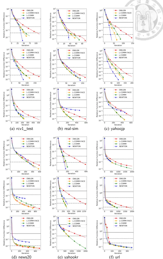
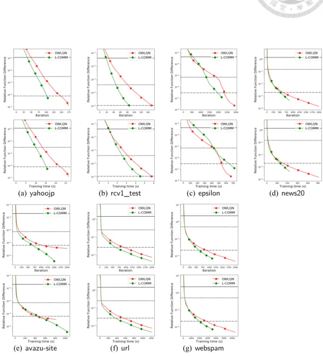
(7) List of Figures 4.1 An illustration of Newton methods for unconstrained and bound-constrained optimization. . . . . . . . . . . . . . . . . . . . . . . . . . . . . . . . . .. 19. 4.2 An illustration of optimization methods for L1 problems. The two horizontal lines indicate suitable range to stop for machine learning applications. .. 19. 6.1 Iteration versus the difference to the optimal value. The horizontal lines indicate when. meets the stopping condition (6.1), with ϵ = 10−2 ,. 10−3 , and 10−4 . . . . . . . . . . . . . . . . . . . . . . . . . . . . . . . . .. 30. 6.2 Comparison of different algorithms by using 32 nodes. Upper: iterations. Lower: running time in seconds. Other settings are the same as Figure 6.1.. 30. D.1 Comparison of different algorithms with 0.1CBest , CBest , 10CBest , respectively from top to below for each data set. We show iteration versus the relative difference to the optimal value. Other settings are the same as in Figure 6.1 . . . . . . . . . . . . . . . . . . . . . . . . . . . . . . . . . . .. 41. D.2 Comparison of different algorithms by using 32 nodes. Upper: iterations. Lower: running time in seconds. Other settings are the same as Figure 6.2.. vi. 42.

(8) List of Tables 4.1 A summary of complexity per iteration for all methods, sorted from cheapest to most expensive. We assume #line-search steps = 1. Only leading terms are presented by assuming m ≪ l and m ≪ n. . . . . . . . . . . . .. 22. 6.1 Data statistics. . . . . . . . . . . . . . . . . . . . . . . . . . . . . . . . . .. 29. vii.

(9) 1 Introduction Given training data (yi , xi ), i = 1, . . . , l with label yi = ±1 and feature vector xi ∈ Rn , we consider L1-regularized linear classification problem. min f (w) ≡ ∥w∥1 + C w. where ∥w∥1 =. "n. j=1. l !. ξ(yi wT xi ),. (1.1). i=1. |wj | and ξ is a differentiable and convex loss function. Here we. consider the logistic loss ξ(z) = log(1 + e−z ). For large applications, (1.1) is often considered because of the model sparsity. Many optimization techniques have been proposed to solve (1.1); see, for example, the comparison in [16]. Generally (1.1) is more difficult than L2-regularized problems because of the non-differentiability. For large-scale data, distributed training is needed. Although for some applications an online method like [10] is effective, for many other applications batch methods are used to more accurately solve the optimization problem. Currently, OWLQN [1], an extension of a limited-memory quasi-Newton method (LBFGS) [8], is the most commonly used distributed method for L1-regularized classification. For example, it is the main linear classifier in Spark MLlib [11], a popular machine learning tool on Spark. OWLQN’s popularity comes from several attributes. First, in a single-machine setting, the compar-. 1.

(10) ison [16] shows that OWLQN is competitive among solvers for L1-regularized logistic regression. Second, while coordinate descent (CD) or its variants [17] are state-of-the-art, they are inherently sequential and are difficult to parallelize in distributed environments. Even if they have been modified for distributed training (e.g., [9]), usually a requirement is that data points are stored in a feature-wise manner. In contrast, as we will see in the discussion in this paper, OWLQN is easier to parallelize and allows data to be stored either in an instance-wise or a feature-wise way. The motivation of this work is to study why OWLQN has been successful and whether we can develop a better distributed training method. We begin with showing in Chapter 2 how OWLQN is extended from the method LBFGS [8]. From that we point out some issues of OWLQN’s direction finding at each iteration. Then in Chapter 3 we extend a recently developed limited-memory common-directions method [7, 14] for L2-regularized problems to the L1 setting. In Chapter 4, through a unified interpretation of methods for L1 problems, we explain why our proposed method is more principled than OWLQN. Although from Chapter 3 our method is slightly more expensive per iteration, the explanation in Chapter 4 and the past results on L2-regularized problems indicate the potential of fewer iterations. For distributed implementations, in Chapter 5 we show that OWLQN and our method have similar communication costs per iteration. Therefore, our method can be very useful for distributed training because the communication occupies a significant portion of the total running time after parallelizing the computation, and our method needs fewer total iterations. The result is confirmed through detailed experiments in Chapter 6. The proposed method has been implemented in MPI-LIBLINEAR ( ). Programs used in this paper are available at. .. 2.

(11) 2 OWLQN: Orthant-Wise Limited-memory Quasi-Newton Method We introduce OWLQN and discuss its issues.. 2.1. Limited-memory BFGS (LBFGS) Method. OWLQN is an extension of the method LBFGS [8] for the following L2-regularized problem. f (w) ≡. wT w + L(w), 2. (2.1). where L(w) ≡ C. l !. ξ(yi wT xi ).. (2.2). i=1. To minimize f (w), Newton methods are commonly used. At the current wk , a direction is obtained by d = −∇2 f (wk )−1 ∇f (wk ).. (2.3). Because calculating ∇2 f (wk ) and its inverse may be expensive, quasi-Newton techniques have been proposed to obtain an approximate direction. d = −Bk ∇f (wk ), where Bk ≈ ∇2 f (wk )−1 .. 3.

(12) BFGS [12] is a representative quasi-Newton technique that uses information from all past iterations and the following update formula. T Bk−1 Vk−1 + ρk−1 sk−1 sTk−1 , Bk = Vk−1. where. Vk−1 ≡ I − ρk−1 uk−1 sTk−1 , sk−1 ≡ wk − wk−1 ,. ρk−1 ≡ 1/(uTk−1 sk−1 ),. uk−1 ≡ ∇f (wk ) − ∇f (wk−1 ),. and I is the identity matrix. To reduce the cost, LBFGS [8] proposes using information from the previous m iterations. From the derivation in [8], the direction d can be efficiently obtained by 2m inner products using columns in the following matrix #. $. P = sk−m , uk−m , . . . , sk−1 , uk−1 ∈ Rn×2m .. (2.4). After obtaining d, a line search ensures the sufficient decrease of the function value. Algorithm 4 in Appendix A summarizes the procedure of LBFGS.. 2.2. Modification from LBFGS to OWLQN. OWLQN extends LBFGS by noticing that instead of the optimality condition. ∇f (w) = 0. 4.

(13) for smooth optimization, for L1 problems in (1.1), w is a global optimum if and only if the projected gradient (PG) is zero.. ∇P f (w) = 0, where for j = 1, . . . , n, ⎧ ⎪ ⎪ ⎪ ⎪ ⎪ ∇j L(w) + 1 ⎪ ⎪ ⎪ ⎪ ⎪ ⎨. if wj > 0, or wj = 0, ∇j L(w) + 1 < 0,. ∇Pj f (w) ≡ ⎪∇j L(w) − 1 ⎪. if wj < 0, or wj = 0, ∇j L(w) − 1 > 0,. ⎪ ⎪ ⎪ ⎪ ⎪ ⎪ ⎪ ⎪ ⎩0. (2.5). otherwise.. The concept of projected gradient is from bound-constrained optimization. If we let. w = w+ − w− , an equivalent bound-constrained problem of (1.1) is. min. w+ ,w−. ! j. wj+. +. !. wj−. +C. j. l ! i=1. ξ(yi (w+ − w− )T xi ). subject to wj+ ≥ 0, wj− ≥ 0, ∀j.. (2.6). Roughly speaking, the projected gradient indicates whether we can update wj by a gradient descent step or not. For example, if. (wk )j = 0 and ∇j L(wk ) + 1 < 0, then (wk )j − α(∇j L(wk ) + 1) > 0, ∀α > 0 5. (2.7).

(14) remain in the orthant of wj ≥ 0 (or wj+ ≥ 0, wj− = 0). On this face f is differentiable with respect to wj and ∇j f (wk ) = ∇j L(wk ) + 1. (2.8). exists. Therefore, if we update wj along the direction of −∇j f (wk ) with a small enough step size, the objective value will decrease. Hence if (2.7) holds, the projected gradient is defined to be the value in (2.8). From the above explanation, the projected gradient roughly splits all variables to two sets: an active one containing elements that might still be modified, and a non-active one including elements that should remain the same. By defining the following active set. A ≡ {j | ∇Pj f (wk ) ̸ = 0},. (2.9). OWLQN simulates LBFGS on the face characterized by the set A, and proposes the following modifications. 1. Because ∇f (wk ) does not exist, the direction d is obtained by using the projected gradient d = −Bk ∇P f (wk ).. (2.10). They apply the same procedure of O(m) vector operations (Algorithm 5 in Appendix A) to get d, but uk−1 is replaced by. uk−1 ≡ ∇L(wk ) − ∇L(wk−1 ). Namely, now Bk is an approximation of ∇2 L(wk )−1 but not ∇2 f (wk )−1 . 2. The search direction is aligned with −∇P f (wk ): dj ← 0 if − dj ∇Pj f (wk ) ≤ 0. 6. (2.11).

(15) Note that after (2.11), we have dA = 0. 3. In line search, they ensure that the new point stays at the same orthant as the original one. ⎧ ⎪ ⎪ ⎪ ⎪ ⎪ max(0, wj + αdj ) ⎪ ⎪ ⎪ ⎪ ⎪ ⎨. wj ← ⎪min(0, wj + αdj ) ⎪ ⎪ ⎪ ⎪ ⎪ ⎪ ⎪ ⎪ ⎪ ⎩0. if wj > 0 or wj = 0, ∇j L(w) + 1 < 0, if wj < 0 or wj = 0, ∇j L(w) − 1 > 0,. (2.12). otherwise.. If we split A to two sets A1 and A2 , A = A1 ∪ A2 , where A1 = {j | wj > 0 or wj = 0, ∇j L(w) + 1 < 0}, A2 = {j | wj < 0 or wj = 0, ∇j L(w) − 1 > 0}, then (2.12) can be written as ⎧ ⎪ ⎪ ⎪ ⎪ ⎪ max(0, wj + αdj ) ⎪ ⎪ ⎪ ⎪ ⎪ ⎨. wj ← ⎪min(0, wj + αdj ) ⎪ ⎪ ⎪ ⎪ ⎪ ⎪ ⎪ ⎪ ⎪ ⎩0. j ∈ A1 , j ∈ A2 ,. (2.13). j∈ / A.. Algorithm 1 summarizes the procedure of OWLQN.. 2.3. Complexity. In one iteration, the following operations are conducted. 1. From ∇L(wk ) = C. l ! i=1. (σ(yi wkT xi ) − 1)yi xi ,. where σ(s) ≡ (1 + exp(−s))−1 , the evaluation of ∇L(wk ) takes O(#nnz), where 7.

(16) Algorithm 1 OWLQN. 1: Given w0 , integer m > 0, and β, γ ∈ (0, 1) 2: w ← w0 3: while true do 4: Calculate ∇P f (w) by (2.5) 5: Calculate the new direction. d ≡ −B∇P f (w) ≈ −∇2 f (w)−1 ∇P f (w) by using information of the previous m iterations (Algorithm 5 in Appendix A) α ← 1, wold ← w while true do Calculate w from wold + αd by (2.12) Calculate the objective value f (w) in (1.1) if f (w) − f (wold ) ≤ γ∇P f (wold )T (w − wold ) break α ← αβ Update P with w − wold and ∇P f (w) − ∇P f (wold ). 6: 7: 8: 9: 10: 11: 12: 13:. #nnz is the number of non-zeros in the training data. 2. At each step of line search, calculating wkT xi , ∀i needs O(#nnz). 3. For obtaining the direction in (2.10), the 2m inner products take O(mn). Therefore, the cost per OWLQN iteration is. (1 + #line-search steps) × O(#nnz) + O(mn).. (2.14). For L2-regularized problems, a trick can be applied to significantly reduce the line-search cost. However, this trick is not applicable for L1-regularized problems because of the max and min operations in (2.12); see more details in Appendix B. Therefore, ensuring a small number of line-search steps is very essential. See Chapter 3.4 for our trick.. 2.4. Issues of OWLQN. Although efficient in practice, OWLQN still possesses several issues in different aspects. To begin, it is known that this method lacks convergence guarantee, though a. 8.

(17) slightly modified algorithm with asymptotic convergence is proposed recently [6]. Next, we discuss several issues related to the construction of the direction.. 2.4.1. Quasi-Newton Direction on the Active Set. Under an active set A, we would like to get a good direction by minimizing the following second-order approximation.. min dA. 1 T 2 dA ∇AA L(wk )dA + ∇PA f (wk )T dA , 2. (2.15). where L(wk ) is defined in (2.2). Thus a quasi-Newton setting should approximate. ∇2AA L(wk )−1 rather than (∇2 L(wk )−1 )AA , but the latter is closer to what OWLQN uses. From (2.9), (2.10), (2.12), OWLQN has the following update direction.. (dk )A = −(Bk ∇P f (wk ))A ≈ −(∇2 L(wk )−1 )AA ∇PA f (wk ).. (2.16). Indeed we observe that using a larger m in OWLQN does not help improve the convergence in terms of number of iterations, while it does for LBFGS on smooth problems, indicating that direction finding in OWLQN is not ideal.. 2.4.2. Alignment with Negative Projected Gradient. After obtaining the direction d by (2.10), OWLQN uses (2.11) to ensure that dj and −∇Pj f (w) have the same sign. This setting leads to that /A dj = 0, ∀j ∈ 9.

(18) and dTA ∇P f (w) ≤ 0, where the former implies that d is on the face A, while the latter tries to have that dA is a descent direction. While both are desired conditions, they are already satisfied without (2.11). From (2.12), only dA is used to update elements in A. Further, if Bk is positive definite, then from (2.16),. ∇P f (wk )T dA = −∇PA f (wk )T (Bk )AA ∇PA f (wk ) < 0. Therefore, an issue is why (2.11) is needed. If the obtained direction is good, the alignment with −∇P f (wk ) may cause worse convergence. On the other hand, we wonder if the issue mentioned in Chapter 2.4.1 makes d a poor direction and hence (2.11) is needed. In Chapter 6, we will thoroughly investigate the effect of aligning the direction with the negative gradient.. 10.

(19) 3 Our Limited-memory Common-directions Algorithm for L1-regularized Classification We extend the limited-memory common-directions method for L2-regularized problems [7, 14] to L1-regularized classification.. 3.1. Past Developments for L2-regularized Problems. To solve (2.1), the method [14] considers an orthonormal basis Pk of all past gradients (called common directions) and obtains the direction d = Pk t by solving the following second-order sub-problem. 1 min ∇f (wk )T Pk t + tT PkT ∇2 f (wk )Pk t, t 2. (3.1). or equivalently, the following linear system:. PkT ∇2 f (wk )Pk t = −PkT ∇f (wk ).. 11. (3.2).

(20) Therefore, in contrast to (2.3) for obtaining a Newton direction, here the direction is restricted to be a linear combination of Pk ’s columns. For (2.1), we can derive. ∇2 f (wk ) = I + CX T Dwk X,. (3.3). where Dw is a diagonal matrix with (Dw )ii = ξ ′′ (yi wT xi ), and X = [x1 , . . . , xl ]T ∈ Rl×n includes all training instances. Then we get. PkT ∇2 f (wk )Pk = PkT Pk + C(XPk )T Dwk (XPk ).. (3.4). Note that PkT Pk = I from the orthonormality of Pk . In [14], they devise a technique to cheaply maintain XPk . Then (3.2) is a linear system of k variables and can be easily solved if the number of iterations is not large. To further save the cost, following the idea of LBFGS in Chapter 2.1, [7] proposes using only information from the past m iterations. They checked several choices of common directions, but for simplicity we consider the most effective one of using past m gradients, past m steps, and the current gradient.. Pk = [∇f (wk−m ), sk−m , . . . , ∇f (wk−1 ), sk−1 , ∇f (wk )] ∈ Rn×(2m+1) .. (3.5). = I. Similar to [3], [7] Because Pk no longer contains orthonormal columns, PkT Pk ̸ T developed an O(mn) technique to easily update Pk−1 Pk−1 to PkT Pk . The cost is about. the same as the 2m vector operations in LBFGS for obtaining the update direction. (See Algorithm 5 in Appendix A.) After solving (3.1) and finding a direction Pk t, they conduct a line search procedure to find a suitable step size. Experiments in [7] show their method is superior to LBFGS.. 12.

(21) To maintain XPk , we need two new vectors. Xsk−1 and X∇f (wk ),. each of which expensively costs O(#nnz). If we maintain Xwk−1 from the function evaluation of the previous iteration, then. Xsk−1 = Xwk − Xwk−1 can be done more cheaply in O(l). Thus X∇f (wk ) is the only expensive operation for maintaining XPk . Therefore, in comparison with LBFGS, at each iteration extra costs include • O(#nnz) for X∇f (wk ) in the matrix XPk , • O(lm2 ) for (XPk )T Dwk (XPk ), • O(mn) for the right-hand side −PkT ∇f (wk ) of the linear system (3.2), • O(m3 ) for solving (3.2), and • O(mn) for computing d = Pk t after obtaining t.. 3.2. Modification for L1-regularized Problems. We propose the following simple modifications. 1. In the sub-problem (3.1), ∇f (wk ) or ∇2 f (wk ) may not exist, so instead we use ∇P f (wk ) and ∇2 L(wk ), respectively. Thus (3.1) becomes 1 min ∇P f (wk )T Pk t + tT PkT ∇2 L(wk )Pk t. t 2. 13. (3.6).

(22) 2. In the matrix Pk of common directions, we use past projected gradients. ∇P f (wk−m ), . . . , ∇P f (wk ) rather than gradients. 3. Similar to the setting in OWLQN, the search direction is aligned with ∇P f (wk ); see (2.11). 4. During line search, the new point stays at the same orthant as the original one; see (2.12). After solving (3.6), the direction used is (Pk t)A . We have. ∇PA f (wk )T (Pk t)A = −∇PA f (wk )T (Pk (PkT ∇2 L(wk )Pk )−1 PkT ∇P f (wk ))A ⎡. ⎤T. ⎡. ⎤. ⎢∇PA f (wk )⎥ ⎢∇P f (wk )⎥ ⎢ ⎥ ⎥ T 2 −1 T ⎢ A = −⎢ ⎥ (Pk (Pk ∇ L(wk )Pk ) Pk ) ⎢ ⎥ ⎣ ⎦ ⎣ ⎦. 0. 0. ≤ 0.. In general, the strict inequality holds, so we have a descent direction. Therefore, following the discussion in Chapter 2.4.2, whether (2.11) should be applied to align the direction with −∇P f (wk ) is an issue. We will conduct a detailed investigation in Chapter 6.1. A summary of the proposed method is in Algorithm 2.. 3.3. Complexity. In Chapters 3.1-3.2, we have discussed operations related to using the common directions. Besides them, function/gradient evaluations are needed. Therefore, the cost per. 14.

(23) iteration is. (2 + #line-search steps) × O(#nnz) + O(lm2 ) + O(mn) + O(m3 ).. (3.7). With m ≪ l and m ≪ n, among the last three terms, O(lm2 ) is the dominant one. In some situations, it may even be the most expensive term in (3.7). For example, if line search terminates in one or two steps and the data set is highly sparse such that #nnz ≈ lm, then lm2 ≈ m × #nnz becomes the bottleneck. Fortunately, the O(lm2 ) term comes from dense matrix-matrix products for constructing the linear system in (3.2). They can be efficiently conducted by using optimized BLAS. Therefore, in general the first term in (3.7) for function/gradient evaluations and X∇P f (wk ) is still the main bottleneck. A comparison between (3.7) and OWLQN’s complexity in (2.14) shows that at every iteration, we need one more O(#nnz) operation for calculating X∇P f (wk ). Therefore, if line search takes only one step per iteration (i.e. #line-search steps = 1; see more details in Chapter 3.4), then we have the following difference between OWLQN and our proposed method: 2 × O(#nnz) versus 3 × O(#nnz).. (3.8). This seems to indicate that each iteration of our method is 50% more expensive than that of OWLQN. However, the three O(#nnz) operations include one X T × (a vector) and two X × (a vector). In Chapter 5 we show that in a distributed environment, the communication cost of X T × (a vector) is much higher. Thus ours and OWLQN have similar communication cost per iteration. Then the higher computational cost may pay off if the number of iterations becomes smaller. 15.

(24) Algorithm 2 Limited-memory common-directions method for L1-regularized problems. 1: Given w0 , integer m > 0, and β, γ ∈ (0, 1) 2: w ← w0 3: while true do 4: Compute ∇P f (w) by (2.5) 5: Solve the sub-problem (3.6) 6: Let the direction be d = P t 7: for j = 1, . . . , n do 8: Align dj with −∇Pj f (w) by (2.11). 16:. α ← 1, wold ← w while true do Calculate w from wold + αd by (2.12) Calculate the objective value f (w) in (1.1) if f (w) − f (wold ) ≤ γ∇P f (wold )T (w − wold ) break α ← αβ Update P and XP. 3.4. Reducing the Number of Line-search Steps. 9: 10: 11: 12: 13: 14: 15:. We have shown in Chapter 3.3 that each line-search step needs O(#nnz) cost for calculating the function value. Because a search starting from α = 1 may result in many steps, we propose using α of the previous iteration as the initial step size. However, to avoid slow convergence of taking too small step sizes, once in several iterations we double the α of the previous iteration as the initial step size.. 3.5. More Details of Limited-memory Common-directions Method. A sketch of the procedure for L1-regularized problems is in Algorithm 2.. 16.

(25) 4 A Unified Interpretation of Methods for L1-regularized Classification We give a unified interpretation of methods for L1-regularized classification. It helps explain firstly why our proposed method is superior to OWLQN, and secondly why OWLQN has been popularly used so far. In Chapter 2.2 we explain that the L1-regularized problem is equivalent to a boundconstrained problem. Most existing methods for bound-constrained optimization conduct the following two steps at each iteration. • Identify a face to be used for getting a direction. • Under a given face, obtain a search direction by unconstrained optimization techniques. The idea is that if we are at the same (or a similar) face of an optimal point, unconstrained optimization techniques can be effectively applied there. In general the identified face is related to non-zero elements of the projected gradient ∇P f (w). For an easy discussion, here we do not touch past developments on face selection; instead, following OWLQN, we consider the set A in (2.9) that consists of all non-zero elements in ∇P f (w). We then focus on obtaining a suitable direction on A satisfying the descent condition (4.2). A framework under this setting is in Algorithm 3. are. 17. Two commonly used search directions.

(26) Algorithm 3 An optimization framework for L1-regularized problems. 1: while true do 2: Compute projected gradient ∇P f (w) by (2.5) 3: Find the set A in (2.9) 4: Get a direction d with /A dj = 0, ∀j ∈ and. 5: 6:. −dTA ∇PA f (w) < 0.. (4.1) (4.2). Align the direction d with −∇P f (w); see (2.11) Line search (and update model parameters) 1. Negative projected gradient direction −∇PA f (w). 2. Newton direction by minimizing (2.15). −∇2AA L(w)−1 ∇PA f (w). Note that a convex loss implies only that ∇2 L(w) is positive semi-definite. For simplicity, we assume it is positive definite and therefore invertible. We note that both directions are on the set A and satisfy the descent condition (4.2) if ∇PA f (w) ̸ = 0. For the Newton direction, because ∇2AA L(w) may be too large to be stored, in linear classification, commonly the special structure in (3.3) (without the identity term) is considered so that a conjugate gradient (CG) procedure is used to solve the linear system. ∇2AA L(w)dA = −∇PA f (w).. (4.3). CG involves a sequence of matrix-vector products and each is performed by. (X:,A )T (Dw (X:,A v)),. where Dw is the same as in (3.3), and v is some vector involved in CG procedure.. 18. (4.4).

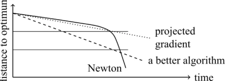
(27) distance to optimum. longer slow-convergence phase because of face selection enter the fast convergence phase unconstrained bound-constrained time. distance to optimum. Figure 4.1: An illustration of Newton methods for unconstrained and bound-constrained optimization.. projected gradient Newton. a better algorithm time. Figure 4.2: An illustration of optimization methods for L1 problems. The two horizontal lines indicate suitable range to stop for machine learning applications. We compare the costs of using the above two directions by assuming that line search terminates in one step. Their complexities per iteration are respectively. 2 × O(#nnz) and (2 + #CG) × O(#nnz). The above cost comes from one function and one gradient evaluation, and for the Newton method, each matrix-vector product in (4.4) requires O(#nnz). One may argue that (4.4) costs O(#nnz × |A|/l) because only |A| columns of X are used. We consider O(#nnz) because, firstly, the analysis is simpler, and secondly, if X is stored in an instance-wise manner, O(#nnz) is needed. Clearly the cost of using a Newton direction is much higher. Unfortunately, the higher cost may not pay off because of the following reasons. 1. The second-order approximation is accurate only near a solution, so a Newton direction in the early stage may not be better than the negative gradient direction. 2. The face A is still very different from that of the convergent point, so a good direction obtained on an unsuitable face is not useful. 19.

(28) The first issue has occurred in unconstrained optimization: A Newton method has fast final convergence, but the early convergence is slow. The second issue, specific to bound-constrained optimization, makes the decision of using an expensive direction or not even more difficult. We give an illustration of Newton methods for unconstrained and bound-constrained optimization in Figure 4.1. For the method of using projected gradient, it not only inherits the slow convergence of gradient descent methods for unconstrained optimization, but also has the issue of face identification. Therefore, the two methods behave like the curves shown in Figure 4.2. Neither is satisfactory in practice. What we hope is something in between: the direction should be better than negative projected gradient, but not as expensive as the Newton direction. The dashed curve in Figure 4.2 is such an example. It is slower than Newton at the final stage, but for machine learning applications, often the optimization procedure can stop earlier, for example, at the region between the two horizontal lines in Figure 4.2. Then the new method is the fastest. To have a method in between, we can either 1. improve the projected gradient direction, or 2. reduce the cost of obtaining a Newton direction. OWLQN is an example. Its quasi-Newton direction needs O(mn) additional cost, but should be better than the projected gradient. Results of OWLQN with similar trends shown in Figure 4.2 have been confirmed empirically in [16]. Thus our analysis illustrates why OWLQN has been a popular method for L1 problems. From the above discussion, many algorithms can be proposed. For example, to reduce the cost of obtaining the Newton direction, we can take fewer CG steps to loosely solve the linear system (4.3). For example, if #CG = m, then the cost per iteration is reduced to (2 + m) × O(#nnz).. 20.

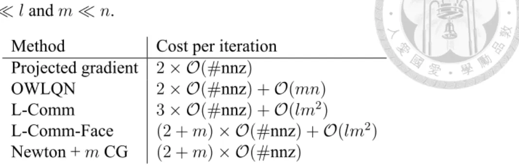
(29) Next we derive the proposed limited-memory common-directions method from the viewpoint of reducing the cost of obtaining a Newton direction. By restricting the direction to be a linear combination of some vectors (i.e., columns in P ), (2.15) becomes 1 min ∇PA f (wk )T (P t)A + ((P t)A )T ∇2AA L(wk )(P t)A . t 2 From (3.4), the quadratic term is. ((P t)A )T ∇2AA L(wk )(P t)A = CtT (X:,A PA,: )T Dwk (X:,A PA,: )t. (4.5). If P has m columns, obtaining X:,A PA,: requires m matrix-vector products, each of which costs O(#nnz). We then solve a linear system of m variables. The setting is similar to that in Chapter 3. Therefore, the cost per iteration is. (2 + m) × O(#nnz) + O(nm) + O(lm2 ) + O(m3 ). We refer to this approach as “L-Comm-Face.” Unfortunately, the cost may be too high. It is as expensive as the Newton method of running m CG steps. We therefore propose an approximation of X:,A PA,: that eventually leads to the proposed method in Chapter 3. If the past m projected gradients have similar active sets to the current ∇P f (wk ), then all m past steps have similar non-zero entries. Therefore,. Pj,: ≈ [0, . . . , 0]. ∀j ∈ /A. implies that X:,A PA,: ≈ XP and (4.5) ≈ tT P T ∇2 L(wk )P t.. (4.6). Thus the method becomes that in Chapter 3 by solving (3.6). The complexity is in (3.7), 21.

(30) Table 4.1: A summary of complexity per iteration for all methods, sorted from cheapest to most expensive. We assume #line-search steps = 1. Only leading terms are presented by assuming m ≪ l and m ≪ n. Method Projected gradient OWLQN L-Comm L-Comm-Face Newton + m CG. Cost per iteration 2 × O(#nnz) 2 × O(#nnz) + O(mn) 3 × O(#nnz) + O(lm2 ) (2 + m) × O(#nnz) + O(lm2 ) (2 + m) × O(#nnz). or if #line-search steps = 1, the complexity becomes. 3 × O(#nnz) + O(lm2 ) + O(mn) + O(m3 ). We refer to the method in Chapter 3 as “L-Comm,” which is an approximation of “LComm-Face” by (4.6). The cost is now close to that of OWLQN. In Chapter 2, we showed some issues of OWLQN in approximating the Newton direction. In contrast, our method is more principled. In Table 4.1, we summarize the complexity per iteration of each discussed method.. 4.1. Quasi-Newton Direction on the Active Set. LBFGS-B [2] is an extension of LBFGS to bound-constrained problems. We include this method in our discussion because we have discussed above that (1.1) is equivalent to a bound-constrained problem (2.6), making this method applicable. At each iteration, LBFGS-B solves a second-order approximation of the original objective on a working set, and then adjust the solution using the original bound constraint. We can view it as a twostage algorithm, where in the first stage, it identifies the active set of the variables, and those outside this set are fixed at this iteration. In the second stage, variables in the active set are treated as unconstrained, and the LBFGS algorithm is applied on this subspace. We treat the active set identification phase as a black-box that we do not give details, as it is. 22.

(31) another research topic beyond the scope of this work, and focus our description on solving ˆ As discussed the unconstrained problem in the subspace. We denote the active set as A. −1 in Chapter 2.4, one should approximate ((∇2 f (wk ))A, but not ((∇2 f (wk ))−1 )A, Â ˆ) Â ˆ,. where we denote f as the objective function of (2.6), which is twice-differentiable, in this section. Therefore, Algorithm 5 in Appendix A cannot be used. Instead, one needs to go back to the LBFGS approximation Hk of ∇2 f (wk ), which is the inverse of Bk described −1 in Chapter 2.1, and compute d = −((Hk )A, Â ˆ ) ∇f (wk )A ˆ by the Sherman-Morrison-. Woodbury formula [13, 15] as the update direction. Finally, after the update direction d is computed, one needs to conduct a line search to ensure feasibility. In our experiment, we will modify LBFGS-B in two places. The first one is the active set identification phase in [2] will be replaced by a simple strategy to consider the non-zero coordinates of the projected gradient (2.5) as the active set. The second modification is that instead of the linear line search to scale d, we use the projected line search approach (2.12). Given m > 0, and the initial estimate θI of ∇2 f (wk ), we define #. $. #. $. #. $. Uk ≡ uk−m . . . uk−1 , Sk ≡ sk−m . . . sk−1 , Wk ≡ Uk θSk ∈ Rn×2m . From [3], the matrix Hk (which is equivalent to Bk−1 , and one can obtain the same formulation through the Sherman-Morrison-Woodbury formula when no active set selection is conducted) is defined as Hk ≡ θI − Wk Mk WkT ,. 23.

(32) where ⎡. ⎢−Dk Mk ≡ ⎢ ⎢ ⎣. Lk. ⎛⎡. ⎤. ⎤⎞. T ⎜⎢sk−m uk−m ⎥⎟. ⎜⎢ ⎜⎢ ⎜⎢ ⎥ , Dk ≡ diag ⎜⎢ ⎜⎢ ⎦ ⎜⎢ θSkT Sk ⎝⎣. LTk ⎥ ⎥. ⎧ ⎪ ⎪ ⎪ ⎪ T ⎪ ⎨(sk−m−1+i uk−m−1+j ). (Lk )i,j ≡ ⎪ ⎪ ⎪ ⎪ ⎪ ⎩0. .. .. sTk−1 uk−1. ⎥⎟ ⎥⎟ ⎥⎟ ⎥⎟ , ⎥⎟ ⎥⎟ ⎦⎠. if i > j . else. Therefore, it is clear that the matrix (Hk )A, Â ˆ is. T θI − (Wk )A,: ˆ Mk ((Wk )A,: ˆ ) ,. and the inverse matrix after the Sherman-Morrison-Woodbury formula is 1 ˜ 1 1 −1 ˜ T ˜ −1 ˜T = I + 2W ((Hk )A, Â ˆ) k (I − Mk Wk Wk ) Mk Wk , θ θ θ. (4.7). ˜ k = (Wk ) ˆ . We then multiply −∇P f (w) by this matrix to obtain the desired where W A,: update direction in the selected coordinates. Note that since the inverse operation in (4.7) is for an 2m × 2m matrix, and m is usually small, we can directly compute the exact inverse in O(m3 ) time.. 24.

(33) 5 Distributed Implementation We show that the proposed method is very useful in distributed environments. To discuss the communication cost, we make the following assumptions. 1. The data set X is split across K nodes in an instance-wise manner: Jr ,. r =. 1, . . . , K form a partition of {1, . . . , l}, and the r-th node stores (yi , xi ) for i ∈ Jr . In addition, XP is split and stored in the same way as X. 2. The matrix P ∈ Rn×2m in (2.4) for OWLQN and P ∈ Rn×(2m+1) in (3.5) for the common-directions method are stored in the same K nodes in a row-wise manner. Thus {1, . . . , n} are partitioned to J¯1 , . . . , J¯K . 3. The model vector w and the projected gradient ∇P f (w) are made available to all K nodes. Communication cost occurs in the following places. 1. Compute ∇L(w) = C where. 6. K 5. ⎡. .. .T. (XJr ,: )T ⎣ ξ′ (yi w .. r=1 .. ⎤. xi ) ⎦. ,. i∈Jr. is the allreduce operation that sums up values from nodes and broadcasts. the result back. The communication cost is O(n).1 2. After obtaining dJ¯r at node r, we need an allgather operation to make the whole direction d available at every node. The communication cost is O(n/K). 3. At each line-search step, to get the new function value, we need an allreduce oper1. The communication cost depends on the implementation of the allreduce operation. Here for easy analysis we use the length of a vector at a local node to be transferred to others as the communication cost.. 25.

(34) ation. f (w) = ∥w∥1 + C. K ! 5. ξ(yi wT xi ).. r=1 i∈Jr. At each node, the sum of local losses is the only value to be communicated, so the cost is O(1). 4. (OWLQN only) Because each node now possesses only a sub-matrix of P , in the procedure of obtaining the search direction d, 2m + 1 distributed inner products are needed. Details are left to Algorithm 7 in Appendix C. For each distributed inner product, the communication cost is O(1). 5. (L-Comm only) To construct the linear system in (3.2), we need the following allreduce operations. The communication cost is O(m2 ). (XP )T Dw (XP ) = P T ∇P f (w) =. K 5 r=1 K 5 r=1. (XJr ,: P )T (Dw )Jr ,Jr (XJr ,: P ) (PJ¯r ,: )T ∇PJ¯r f (w).. A rough estimate of the communication cost is. OWLQN: O(n) + O(n/K) + O(1) + (2m + 1) × O(1), L-Comm: O(n) + O(n/K) + O(1) + O(m2 ). For large and sparse data, n ≫ m2 . The dominant term is O(n), so the two methods have similar communication costs. This situation is different from that of computational complexity. In (3.8), we state that our method may be 50% more expensive than OWLQN for computing X∇P f (w). However, this operation does not involve any communication because a local node simply calculates XJr ,: ∇P f (w) to update the local XJr ,: P . Thus our method is useful in a distributed setting. Its higher cost per iteration becomes a less. 26.

(35) serious concern because the computation is parallelized and the communication may take a significant portion of the total time. In Appendix C, we provide details of distributed versions of OWLQN and L-Comm in Algorithm 6 and Algorithm 8, respectively.. 27.

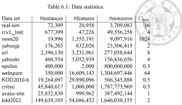
(36) 6 Experiments We consider binary classification data sets listed in Table 6.1.1 We implement all methods under the framework of LIBLINEAR [4] (for Chapter 6.1) or Distributed LIBLINEAR (for Chapter 6.2). OpenBLAS2 is used for dense vector/matrix operations. We check the convergence of optimization methods by showing the number of iterations or running time versus the relative difference to the optimal function value f (wk ) − f ∗ , f∗ where f ∗ is an approximate optimal objective value by accurately solving the optimization problem. For the regularization parameter C, we select CBest that achieves the best cross validation accuracy. More details and results of using other C values are in Appendix D.1.. 6.1. Comparisons on Number of Iterations. From Chapter 4, both OWLQN and L-Comm are designed to approximate the Newton direction because conceptually better directions should lead to a smaller number of iterations. Without considering the cost per iteration, we begin with checking this result by comparing the following methods discussed in Chapter 4. • 1. [1]: We consider m = 10.. All data sets except. and. are from. 2. 28.

(37) Table 6.1: Data statistics. Data set. #instances 72,309 677,399 19,996 176,203 2,396,130 460,554 400,000 350,000 19,264,097 45,840,617 25,832,830 149,639,105. #features 20,958 47,226 1,355,191 832,026 3.231,961 3,052,939 2,000 16,609,143 29,890,096 1,000,000 999,962 54,686,452. #nonzeros 3,709,083 49,556,258 9,097,916 23,506,415 277,058,644 156,436,656 800,000,000 1,304,697,446 566,345,888 1,787,773,969 387,492,144 1,646,030,155. CBest 16 4 1024 2 8 4 0.5 64 0.5 0.5 1 2. •. : We use information from past 10 iterations as common directions.. •. : The proposed method in Chapter 3, which according to the discussion in Chapter 4 is an approximation of. •. .. : We run 50 CG steps at each iteration. This setting simulates the situation where the full Newton direction on the face is obtained.. All these methods find a direction on the face decided by the project gradient and conduct line search to find a suitable step size.3 Comparison results are in Figure 6.1 and Appendix D.2. Three horizontal lines are plotted to show some reasonable stopping condition min(l+ , l− ) ∥∇P f (w)∥ ≤ ϵ , ∥∇P f (0)∥ l. (6.1). where l+ ≡ |{i|yi = 1}| and l− ≡ |{i|yi = −1}|. We make the following observations. •. is generally among the best, but not always (e.g.,. ). A possible. explanation is that these methods are not compared under a fixed face. Instead, the methods go through different face sequences. Thus a method of using a better direction locally may not be the best globally. Nevertheless, the overall good performance of 3. indicates that one should consider a better direction under. A backtracking line search with initial step size = 1 is used.. 29.

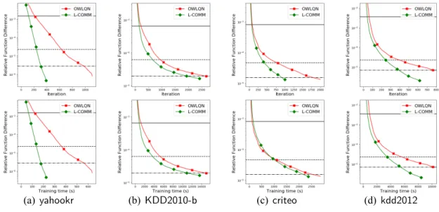
(38) (a). (b). (c). (d). Figure 6.1: Iteration versus the difference to the optimal value. The horizontal lines indicate when meets the stopping condition (6.1), with ϵ = 10−2 , 10−3 , and 10−4 .. (a). (b). (c). (d). Figure 6.2: Comparison of different algorithms by using 32 nodes. Upper: iterations. Lower: running time in seconds. Other settings are the same as Figure 6.1. any given face if possible. Further, the shape of. ’s curve is close to the. illustration in Figure 4.1 for smaller C (see Appendix D.1), but for larger C, it is not that close. An explanation is that for larger C, the problem is more difficult and is still under the stage of finding a suitable face. • The convergence of. is generally very good, indicating its use of. common directions to approximate the Newton direction is very effective. •. is an excellent approximation of ilar or slightly inferior to that of. • In general,. . Its convergence is sim.. has the worst convergence speed in terms of iterations. 30.

(39) Overall results are consistent with the analysis in Chapter 4. If we also consider the cost per iteration,. and. are not practical. From Table 4.1 each their. iteration is O(m) times more than that of. and. , and their saving on the. number of iterations is not enough to compensate for the higher cost per iteration. We expect. to be the best in terms of running time because it needs fewer. iterations than. and requires only comparable cost per iteration. This will be. confirmed in Chapter 6.2.. 6.2. Timing Comparison of Distributed Implementations. We consider a distributed implementation of [5]. We use 32. and. using OpenMPI. nodes on AWS with 1Gbps network bandwidth. The strategy. in Chapter 3.4 is applied to possibly reduce the number of line-search steps. Since the focus is on comparing distributed implementations, we do not parallelize computation at each local node. Results in Figure 6.2 show that. always converges faster than. in. terms of iterations, which is consistent with the results in Chapter 6.1. Next we present running time also in Figure 6.2. In Chapters 3-4 we have indicated that more expensive than. is slightly. per iteration, so the smaller number of iterations may not. lead to shorter total time. However, the analysis in Chapter 5 shows that both methods have similar communication cost per iteration. Because in a distributed setting the communication may take a large portion of the total running time, we observe that figures for timing comparisons are very close to those for iterations. An exception is. , which. has a relatively smaller number of features. Thus, for this set the communication cost is insignificant among the total cost. Overall, this experiment shows that the proposed method is more efficient than. in a distributed environment.. 31.

(40) 7 Conclusions In this work we present a limited-memory common-directions method for L1-regularized classification. The method costs slightly more than OWLQN per iteration, but may need much fewer iterations. Because both methods’ communication is proportional to the number of iterations, our method is shown to be faster than OWLQN in distributed environments. In addition, we give a unified interpretation of methods for L1-regularized classification. From that we see our method is a more principled approach than OWLQN.. 32.

(41) A. Derivation of the Direction Used in LBFGS. By using only the information from the last m iterations, the definition of Bk in BFGS becomes the following in LBFGS.. T T · · · Vk−m B0k Vk−m · · · Vk−1 Bk = Vk−1. (A.1). T T + ρk−m Vk−1 · · · Vk−m+1 sk−m sTk−m Vk−m+1 · · · Vk−1. + · · · + ρk−1 sk−1 sTk−1 . Note that in BFGS, B0k is a fixed matrix, but in LBFGS, B0k can change with k, provided its eigenvalues are bounded in a positive interval over k. A common choice is. B0k =. sTk−1 uk−1 I. uTk−1 uk−1. (A.2). By expanding (A.1), dk can be efficiently obtained by O(m) vector operations as shown in Algorithm 5 in Appendix A. The overall procedure of LBFGS is summarized in Algorithm 4 in Appendix A.. 33.

(42) Algorithm 4 LBFGS. 1: Given w0 , integer m > 0, and β, γ ∈ (0, 1) 2: w ← w0 3: while true do 4: Calculate ∇f (w) 5: Calculate the new direction. d ≡ − B∇f (w) ≈ −∇2 f (w)−1 ∇f (w) by using information of the previous m iterations (Algorithm 5) Calculate ∇f (w)T d α ← 1, wold ← w while true do w ← wold + αd Calculate the objective value f (w) in (2.1) if f (w) − f (wold ) ≤ γ∇f (wold )T (w − wold ) break α ← αβ 14: Update P with w − wold and ∇f (w) − ∇f (wold ) 6: 7: 8: 9: 10: 11: 12: 13:. Algorithm 5 LBFGS Two-loop recursion. 1: q ← −∇f (w) 2: for i = k − 1, k − 2, . . . , k − m do 3: αi ← sTi q/sTi ui 4: q ← q − αi ui. 5: r ← (sTk−1 uk−1 /uTk−1 uk−1 )q 6: for i = k − m, k − m + 1, . . . , k − 1 do 7: βi ← uTi r/sTi ui 8: r ← r + (αi − βi )si 9: d ← r. 34.

(43) B. Line Search in Algorithms for L2-regularized Problems Here we present the trick mentioned in Chapter 2.3 in the paper. At each line search. iteration, we obtain wT xi , dT xi , ∀i first, and then use O(l) cost to calculate (w + αd)T xi = wT xi + αdT xi , ∀i. Because wT xi can be obtained from the previous iteration, dT xi is the only O(#nnz) operation needed. The line search cost is reduced from. #line-search steps × O(#nnz) to 1 × O(#nnz) + #line-search steps × O(l). This trick is not applicable to L1-regularized problems because the new point is no longer w + αd.. 35.

(44) C. More on the Distributed Implementation. C.1 Complexity The distributed implementation mentioned in Chapter 5 is shown in Algorithm 8. The complexity is (2 + #line-search steps) × O(#nnz) + O(lm2 ) + O(mn) + O(m3 ) K. 36.

(45) Algorithm 6 A distributed implementation of OWLQN. 1: for k = 0, 1, 2, . . . do 2: Compute ∇P f (w) by (2.5) and ⎡. ⎤. .. . ⎢ ⎥ 5K T ⎢ ′ ⎥ ∇L(w) = C r=1 (XJr ,: ) ⎢ξ (yi wT xi )⎥ ⎣ ⎦ .. .. .. i∈Jr. ◃ O(#nnz/K); O(n) comm. 3: Compute the search direction dJ¯r , r = 1, . . . , K by Algorithm 7 ◃ O(nm/K); O(m) comm. 4: An allgather operation to let each node has ⎡. ⎤. dJ¯ ⎢ .1⎥ . ⎥ d=⎢ ⎣ . ⎦ dJ¯K. 5: 6: 7: 8: 9:. for j = 1, . . . , n do Align dj with −∇Pj f (w) by (2.11). α ← 1, wold ← w while true do Calculate w from wold + αd by (2.12) and f (w) = ∥w∥1 + C. 10: 11: 12: 13: 14:. 5K. r=1. !. i∈Jr. ξ(yi wT xi ). if f (w) − f (wold ) ≤ γ∇P f (wold )T (w − wold ) break α ← αβ sk ← w − wold , uk ← ∇f (w) − ∇f (wold ) Remove 1st column of S and U if needed and 7. 8. S ← S sk , 15:. ◃ O(n/K) comm.. ρk ←. 6K. T r=1 (uk )J¯r (sk )J¯r. 7. ◃ O(#nnz/K); O(1) comm.. U ← U uk. 8. ◃ O(n/K); O(1) comm.. 37.

(46) Algorithm 7 Distributed OWLQN Two-loop recursion 1: if k = 0 return dJ¯r ← −∇PJ¯ f (w) r. 2: for r = 1, . . . , K do in parallel 3: qJ¯r ← −∇PJ¯ f (w). ◃ O(n/K). r. 4: for i = k − 1, k − 2, . . . , k − m do 5: Calculate αi by. αi ← 6: 7:. 6K. T r=1 (si )J¯r qJ¯r. ρi ◃ O(n/K); O(1) comm.. for r = 1, . . . , K do in parallel qJ¯r ← qJ¯r − αi (ui )J¯r. 8: Calculate. uTk−1 uk−1 ←. ◃ O(n/K) K 5 r=1. (uk−1 )TJ¯r (uk−1 )J¯r ◃ O(n/K); O(1) comm.. 9: for r = 1, . . . , K do in parallel 10: rJ¯r ← uT ρk−1 rJ¯r u. ◃ O(n/K). k−1 k−1. 11: for i = k − m, k − m + 1, . . . , k − 1 do 12: Calculate βi by 6K. βi ←. 13: 14:. T r=1 (ui )J¯r rJ¯r. ρi ◃ O(n/K); O(1) comm.. for r = 1, . . . , K do in parallel rJ¯r ← rJ¯r + (αi − βi )(si )J¯r return dJ¯r ← rJ¯r , r = 1, . . . , K. ◃ O(n/K). 38.

(47) Algorithm 8 Distributed limited-memory common-directions method. 1: while true do 2: Compute ∇P f (w) by (2.5) and ⎡. ⎤. .. . ⎢ ⎥ 5K ⎥ T ⎢ ′ ∇L(w) = C r=1 (XJr ,: ) ⎢ξ (yi wT xi )⎥ ⎣ ⎦ .. .. .. i∈Jr. 3: 4:. 7. 8. 7. PJr ,: ← PJr ,: ∇PJr f (w) ; 5:. Calculate. (XP )T Dw (XP ) =. 7:. Solve. 9. 8. UJr ,: ← UJr ,: XJr ,: ∇P f (w). 5K. r=1. −P T ∇P f (w) = − 6:. ◃ O(#nnz/K); O(n) comm. ◃ O(#nnz/K). Calculate XJr ,: ∇P f (w) Remove 1st column of P and U if needed and. (UJr ,: )T (Dw )Jr ,Jr UJr ,: ◃ O(lm2 /K), O(m2 ) comm.. 5K. r=1. (PJ¯r ,: )T ∇PJ¯r f (w) ◃ O(mn/K); O(m) comm.. :. (XP )T Dw (XP ) t = −P T ∇P f (w). ◃ O(m3 ). Let the direction be 7. 8T. d = P t = PJ¯1 ,: t, . . . , PJ¯K ,: t 8: 9: 10: 11: 12:. for j = 1, . . . , n do Align dj with −∇Pj f (w) by (2.11). α ← 1, wold ← w while true do Calculate w from wold + αd by (2.12) and f (w) = ∥w∥1 + C. 13: 14: 15: 16:. ◃ O(mn/K); O(n/K) comm.. 5K. r=1. !. i∈Jr. ξ(yi wT xi ). if f (w) − f (wold ) ≤ γ∇P f (wold )T (w − wold ) break α ← αβ Remove 1st column of P and U if needed and 7. 8. P ← P w − wold ;. 7. ◃ O(#nnz/K); O(1) comm.. 8. UJr ,: ← UJr ,: XJr ,: (w − wold ). 39.

(48) D. More Experiments. The data sets used in this section are shown in Table 6.1.. D.1 More Results by Using Different C Values In Figure D.1, we present more results with. C = {0.1CBest , CBest , 10CBest }, where CBest is the value to achieve the highest cross validation accuracy. The results are similar to CBest presented in Chapter 6, but we observe that. converges slowly. in larger C cases.. D.2 More Results on Distributed Experiments In Figure D.2, we present more data sets for the distributed experiments. All settings are the same as in Chapter 6.. 40.

(49) (a). (d). (b). (c). (e). (f). Figure D.1: Comparison of different algorithms with 0.1CBest , CBest , 10CBest , respectively from top to below for each data set. We show iteration versus the relative difference to the optimal value. Other settings are the same as in Figure 6.1. 41.

(50) (a). (e). (b). (c). (f). (d). (g). Figure D.2: Comparison of different algorithms by using 32 nodes. Upper: iterations. Lower: running time in seconds. Other settings are the same as Figure 6.2.. 42.

(51) Bibliography [1] G. Andrew and J. Gao. Scalable training of L1-regularized log-linear models. In ICML, 2007. [2] R. H. Byrd, P. Lu, J. Nocedal, and C. Zhu. A limited memory algorithm for bound constrained optimization. SIAM J. Sci. Comput., 16:1190–1208, 1995. [3] R. H. Byrd, J. Nocedal, and R. B. Schnabel. Representations of quasi-Newton matrices and their use in limited memory methods. Math. Program., 63:129–156, 1994. [4] R.-E. Fan, K.-W. Chang, C.-J. Hsieh, X.-R. Wang, and C.-J. Lin. LIBLINEAR: a library for large linear classification. JMLR, 9:1871–1874, 2008. [5] E. Gabriel, G. E. Fagg, G. Bosilca, T. Angskun, J. J. Dongarra, J. M. Squyres, V. Sahay, P. Kambadur, B. Barrett, A. Lumsdaine, R. H. Castain, D. J. Daniel, R. L. Graham, and T. S. Woodall. Open MPI: Goals, concept, and design of a next generation MPI implementation. In European PVM/MPI Users’ Group Meeting, pages 97–104, 2004. [6] P. Gong and J. Ye. A modified orthant-wise limited memory quasi-Newton method with convergence analysis. In ICML, 2015. [7] C.-P. Lee, P.-W. Wang, W. Chen, and C.-J. Lin. Limited-memory common-directions. 43.

(52) method for distributed optimization and its application on empirical risk minimization. In SDM, 2017. [8] D. C. Liu and J. Nocedal. On the limited memory BFGS method for large scale optimization. Math. Program., 45(1):503–528, 1989. [9] D. Mahajan, S. S. Keerthi, and S. Sundararajan. A distributed block coordinate descent method for training l1 regularized linear classifiers. JMLR, 2017. [10] H. B. McMahan, G. Holt, D. Sculley, M. Young, D. Ebner, J. Grady, L. Nie, T. Phillips, E. Davydov, D. Golovin, S. Chikkerur, D. Liu, M. Wattenberg, A. M. Hrafnkelsson, T. Boulos, and J. Kubica. Ad click prediction: a view from the trenches. In KDD, 2013. [11] X. Meng, J. Bradley, B. Yavuz, E. Sparks, S. Venkataraman, D. Liu, J. Freeman, D. Tsai, M. Amde, S. Owen, D. Xin, R. Xin, M. J. Franklin, R. Zadeh, M. Zaharia, and A. Talwalkar. MLlib: Machine learning in Apache Spark. JMLR, 17:1235–1241, 2016. [12] J. Nocedal and S. Wright. Numerical Optimization. Springer, second edition, 2006. [13] J. Sherman and W. J. Morrison. Adjustment of an inverse matrix corresponding to a change in one element of a given matrix. The Annals of Mathematical Statistics, 21(1):124–127, 1950. [14] P.-W. Wang, C.-P. Lee, and C.-J. Lin. The common directions method for regularized empirical loss minimization. Technical report, National Taiwan University, 2016. [15] M. A. Woodbury. Inverting modified matrices. Technical Report 106, Statistical Research Group, Princeton University, 1950.. 44.

(53) [16] G.-X. Yuan, K.-W. Chang, C.-J. Hsieh, and C.-J. Lin. A comparison of optimization methods and software for large-scale l1-regularized linear classification. JMLR, 11:3183–3234, 2010. [17] G.-X. Yuan, C.-H. Ho, and C.-J. Lin. An improved GLMNET for l1-regularized logistic regression. JMLR, 13, 2012.. 45.

(54)