Power-Efficient Geographic Routing for MANETs

全文

(1)Power-Efficient Geographic Routing for MANETs Workshop: B. Workshop on Computer Networks. Luan Lan and Hsu Wen-Jing. ABSTRACT We present a location-aware routing protocol called MGPSR (Modified Greedy Perimeter Stateless Routing) for Mobile Ad Hoc Networks. MGPSR offers the crucial correctness guarantee of the well known Greedy Perimeter Stateless Routing (GPSR) protocol; moreover, it possesses two additional attractive properties: (1) the modified Greedy forwarding scheme balances between the transmission power consumption and the transmission latency, and (2) the modified perimeter forwarding makes use of the localized Delaunay graph which offers higher connectivity and provides a path with fewer hops. The algorithm works in a distributed and dynamic fashion with low overhead. In contrast to pure topology-based protocols, MGPSR does not drain the network bandwidth by imposing large amount of protocol traffic. The new algorithm is evaluated both theoretically and empirically. Extensive simulations have demonstrated that the MGPSR outperforms the GPSR protocol.. First Author (Contact Author):. Second Author:. Luan Lan. Hsu Wen-Jing. Year 4, School of Computer Engineering. Assoc Professor. Nanyang Technological University. Deputy Director, MRC School of Computer Engineering. Address: Hall 2 – Block 9 – 2 – 133. Nanyang Technological University. Nanyang Technological University Singapore 639798 Cellular: 65-93856973. Tel: 65-67904597 Email: [email protected]. Email: [email protected]. Keywords: Mobile Ad Hoc Networks, Routing Protocols, Power-efficient, Transmission Latency, Planarization, Greedy Forwarding, Delaunay Graph, GPSR etc..

(2) Power-Efficient Geographic Routing for MANETs Luan Lan and Hsu Wen-Jing School of Computer Engineering Nanyang Technological University Singapore 639798. In MANETs, autonomous wireless mobile hosts double as a router to transport information collaboratively. Routing is generally multi-hop in that a given destination node may be beyond the transmission range of the source node and thus depends on intermediate stations to forward packets. Since the topology in an ad hoc network changes unpredictably and frequently, an efficient routing protocol needs to determine high quality routes whilst holding the maintenance overhead to a minimum. Many protocols have been proposed (cf. References for samples), which can be broadly classified into topology-based routing protocols and position-based routing protocols. Metrics for evaluating the quality of a protocol are transmission latency, delivery energy, success rate and so forth. The objective of this paper is to address the trade-offs between energy consumption and latency. The following gives a brief review of major existing approaches. The reader is referred to [34] for more comprehensive account.. ABSTRACT We present a location-aware routing protoc ol called MGPSR (Modified Greedy Perimeter Stateless Routing) for Mobile Ad Hoc Networks. MGPSR offers the crucial correctness guarantee of the well known Greedy Perimeter Stateless Routing (GPSR) protocol; moreover, it possesses two additional attractive properties: (1) the modified Greedy forwarding scheme balances between the transmission power consumption and the transmission latency, and (2) the modified perimeter forwarding makes use of the localized Delaunay graph which offers higher connectivity and provides a path with fewer hops. The algorithm works in a distributed and dynamic fashion with low overhead. In contrast to pure topology-based protocols, MGPSR does not drain the network bandwidth by imposing large amount of protocol traffic. The new algorithm is evaluated both theoretically and empirically. Extensive simulations have demonstrated that the MGPSR outperforms the GPSR protocol. 1.. Topology-based routing protocols use the link information to direct packet forwarding. A classical taxonomy further divides this group into: proactive, reactive and hybrid protocols. Link-State and Distance-Vector are two commonly adopted algorithms. Proactive protocols such as EXBF [9], DSDV [32], OLSR [21], and STAR [17] continually update route entries in order to minimize route selection delays; however, because all globally available links including those not currently in use are kept, wasteful updates and bandwidth overhead are incurred. Several cluster based ad-hoc routing protocols, like Landmark Hierarchy [43], Partialknowledge Spine Routing (PSR) [39], CEDAR [40], and CGSR [10] also belong to this category. In contrast, the reactive protocols initiate the routing. INTRODUCTION. 1.1 MANETs and Routing Protocols The widespread availability of wireless communication devices has st imulated the research of self-organizing networks in recent years. In places where there is little or no pre-established communication infrastructure, the technology of Mobile Ad Hoc Networks (or MANETs for short) allows mobile applications to maintain dynamic connections. Applications of such a network include mobile conferencing, emergency services, personal area networks, Bluetooth, sensor dust and military command and communications [34].. 1.

(3) discovery and maintenance in an on-demand manner, only preceding the transmission of a packet. The overhead is significantly lessened at the expense of routing delay time. DSR [5], AODV [33], TORA [31] , and GEO-TORA [26] have all contributed to repertoire of the on-demand request and reply schemes. Since each host has minimal information about the entire topology, most algorithms of this class employ flooding over the network to find the path to a destination. Consequently, route discovery and update could lead to significant volume of network traffic especially when the topology undergoes rapid changes. Hybrid protocols like ZRP [18] combine local proactive routing and global reactive routing to achieve higher scalability. However, since they still require cached network paths, the amount of topological changes may not exceed a limit within a period of time.. synchronization is required for both, and failures due to location errors are inevitable. Moreover, the actual flooding, though somewhat constrained, still consumes too much bandwidth and power. As node density increases, the shortest path between the source and destination corresponds more closely to the straight line connecting them. Based on this premise, a node can make a locally optimal, greedy choice of the next hop, which is the neighbor geographically lying in the general direction to the recipient. GPSR The prime example of effective yet localized location-aware protocol is proposed by Karp and Kung in [24]: the Greedy Perimeter Stateless Routing (GPSR) protocol, which is nearly stateless and requires propagation of topology information for only a single hop. Nodes acquire one-hop topological information through beacon message exchanges. Their routing method consists of two modes, namely the greedy forwarding and perimeter forwarding. GPSR guarantees the delivery of any packet in static network if a path exists. The proposal proves to be very elegant and practical.. Position-based protocols, or location-aware protocols exploit the location information (in the form of coordinates) to alleviate the shortcomings of topology-based routing. The routing decision relies on the destination’s position to select the next forwarding host among the sender’s one-hop neighbors (i.e. hosts that lie in the transmission range). Routing a packet typically comprises two distinct phases: (1) discovering the position of the destination, and (2) the actual forwarding, based on the proximate location information.. Our research focuses on improving GPSR in following aspects: (a) routing optimization in greedy mode to strike a balance between energy consumption and transmission delay, and (b) the construction and maintenance of dynamic connectivity information for better route quality in perimeter mode. The second aspect has been studied in [15], while the first has received little attention. Herein we present a novel scheme called the Modified Greedy Perimeter Stateless Routing (MGPSR) protocol. The quality of routing is secured by inheriting the correctness guarantee of GPSR; the density-based greedy forwarding redefines the route selection criteria to conserve energy; the protocol does not drain the network bandwidth by imposing large amount of protocol traffic. In fact, the protocol traffic over the entire network grows linearly with the number of mobile nodes, which is one of the most scalable among known schemes.. Each node determines its own location through positioning services like GPS [6] and obtains the location of the destination through a location service (see [22] for a survey of location services). One such system developed is GLS with Geographic Forwarding [27]. Predefined identifier ordering and spatial hierarchy impose an upper-bound on the number of the intermediate hops which, in turn, ensures a low latency address resolution process. Restricted directional flooding and Greedy forwarding are two main branches beneath positionbased routing strategy. LAR [25] and DREAM [2], as examples of restricted directional flooding protocols , attempt to confine the flooding to a smaller request zone containing the destination. Unfortunately, time. 2.

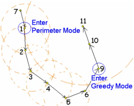
(4) 1.2 Notions. and returns to the greedy mode when it reaches a node closer to the destination than the perimeter mode entrance point. Karp and Kung demonstrated that these two methods can ensure the delivery of a packet in static network if there is an existing route.. The following conventions are adopted throughout the paper: d(x, y): The Euclidean distance between node x and node y. xy : The edge connecting node x and node y.. C(x, y): The circle that has xy as its diameter. R: The one-hop broadcast radio range initially fixed for all nodes, which may not necessarily equal to the actual transmission radius. LA(x): The neighborhood of node x, i.e. the circular region within radius R with x at the center. 1.3 Organization Figure 2.1 Switching between Greedy and Perimeter Mode. The rest of the paper is organized as follows. Section 2 surveys other closely related work. Section 3 presents our algorithm for the local approximation of the Delaunay Triangulation. It uses Gabriel’s Graphs (denoted as GG for short) as its starting point. Section 4 details the density-based greedy forwarding strategy. Section 5 examines various properties of the MGPSR and compares it with GPSR via simulations. Section 6 highlights the main features of our approach and points out useful directions for future research. 2.. Note that, to avoid circular tours caused by crossing edges, the underlying graph must be planar for perimeter forwarding. Karp and Kung have proposed to use a planarization♦ scheme that results in a special type of planar graphs named Relative Neighborhood graph (or RNG for short)[42]. An alternative called Gabriel’s Graph (or GG for short) [16] was also suggested. Assuming uniform distribution, the computational overhead for adding or eliminating one edge per node is O(1) for both graphs (cf. [28]). Definitions of RNG and GG are given in Appendix A.. PRELIMINARIES. 2.1 GPSR Protocol in Detail In the GPSR protocol [24], the sender of a packet incorporates the approximate position of the recipient into the packet. Whenever possible, a message will be routed nearer to its destination by greedy forwarding, i.e. forwarding the packet to the single-hop neighbor that makes the most progress towards the destination. The greedy routing may fail to find a path, even though one does exist. At any node, where none of its neighbors is closer to the destination, the perimeter forwarding will be applied, which essentially moves the packet around the void area by stipulating the right-hand rule (viz., rotate counterclockwise to get the first neighbor as the next hop) and the face change rule (Figure 2.1). A packet enters this recovery mode when arriving at a local maximum. 2.2 Delaunay Triangulation (DT) Both RNG and GG are rather sparse graphs. In [13], it was shown that, these graphs are more vulnerable to disconnection or partition in the presence of link failures. Therefore, it is desirable to design a denser planar graph which ideally (a) incurs low protocol overhead during construction and maintenance, and (b) incurs low operational cost in perimeter forwarding.. ♦. Links on the graph G will be examined (and pruned if necessary) to ensure that the resulting graph G’ is planar. The process is referred to as “planarization”, which maps G to planar graph G’.. 3.

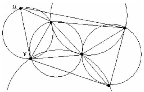
(5) 2.2.1 Delaunay Triangulation (Global DT) ♦ The Delaunay Triangulation (or DT for short) has been long regarded as a good spanner of a given set of nodes (refer to Appendix A for definition). It is also well known that DT is a superset of GG which in turn, is a superset of RNG [35]. The traditional algorithms for the construction of DT are not suitable for distributed environment because they either require prior knowledge of the entire topology or employ incremental edge-flipping strategies that propagate an unbounded number of hops. With power constraints, ti is impractical for all nodes to obtain and maintain positional information over a large area.. response to decommissioning of old links, or instatement of new ones would be serious especially under high mobility. In [15] the issues of transmission power are not addressed either. 3. LOCALIZED CONSTRUCTION. DELAUNAY. DIAGRAM. The local construction could be generalized from one-hop to k-hops. The larger value k is, the better approximation to DT will result with correspondingly larger overhead. In this section, we only briefly describe the construction of one-hop Local Delaunay Diagram. Detailed proofs are referred to [28].. 2.2.2 Localized Delaunay Diagram (LDD) We developed an approximation to DT, which is feasible for local construction while ensuring the planarity, reachability and scalability.. 3.1 One-Hop Local Delaunay Diagram based on GG with Additional Crossing Edge Elimination (1+-GLDD) Algorithm Definition Let u and v be any two nodes in a set of given nodes V such that d (u , v ) ≤ R . Define the union of LA(u) and LA(v) as LAU(u,v). A triangle with vertices u and v is said to be a 1-hop Local Delaunay Triangle (1-LDT) if and only if its circumcircle contains no other nodes than its vertices within LAU(u,v).. Definition Given a set of nodes V and a length R, a 1-hop Localized Delaunay Diagram of V contains all Delaunay edges that have a length ≤ R. Recently, a parallel study [15] by Gao et al. described similar concepts and brought forward a distributed algorithm to construct such a graph. It works as follows. Each node acquires the posit ion of its neighbors and computes the Delaunay triangulation in the one-hop circle. Since the local construction at different nodes could be inconsistent, additional information propagation is performed. Each node broadcasts its local Delaunay triangulation results to its immediate neighbors. A local DT edge uv is deleted if it does not belong to the local Delaunay graph of any mutual neighbor w of u and v .. Definition An edge uv is in 1-GLDD if (a) it is in GG, or (b) there is a node w in C(u,v) such that ∆ uvw is a 1-LDT. To achieve the required testing, two mobile hosts u and v may obtain the knowledge about LAU(u,v) by beaconing and exchange of neighborhood tables. An illustration is given in Figure 3.1.. One of the drawbacks lies in the fact that, to validate the edge uv when node v has just moved to u ’s one-hop area, node u must wait until all common neighbors firstly become aware of v and recalculated local Delaunay Diagrams from them are received in the worst case. During that particular interval, the network topology may become invalid and crossing edges are temporarily possible. The problem of slow. ♦. We prefix DT with “Global” to distinguish it from the Local DT discussed shortly.. Figure 3.1 1-GLDD Graph 4.

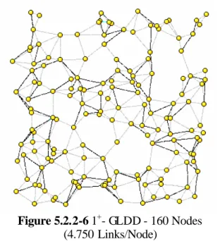
(6) on limited battery power supply. It is commonly known that battery technology is not likely to progress as fast as computing technologies. Hence, how to lengthen the lifetime of batteries by algorithms that take into consideration the energy conservation while still maintaining a high packet success rate and low packet delay opens new horizons for research.. (1) The inner circle is C(u,v) with diameter uv . The shaded area (including C(u,v)) is LAU(u,v), union of u and v’s one-hop radio area. (2) uv is in 1-GLDD since it is in GG. (3) uv is not in GG (C(u,v) is not empty). However, because the circumcircle of ∆ uvw does not contain any node from LAU(u,v), uv is in 1-GLDD.. Energy is mainly consumed in (a) transmitting or forwarding data to recipient or (b) maintaining the topological information in response to the changing network. The transmission success rate is largely dependent on the freshness of topological knowledge kept by nodes, and is thus constrained by the limited power capability. Given the energy budget, the node behavior could also affect the transmission latency in two ways: First, the more link information is made available, the less effort and better quality a route can be established; the routes stored are also more likely to be valid with frequent updates. Second, among several routing options, forwarding to the nearest hop would reduce the transmission distance and thereby conserve power. Nevertheless, this may involve more intermediate hops , and thus the nodal delay, a major contributor of latency rises.. In some rare cases, crossing edges are still possible after 1-GLDD algorithm is applied. It is proved that the only possible scenario can be avoided by nocrossing heuristic proposed in [28]. The resulting algorithm is hereby referred to as 1+-GLDD, where the “+” sign denotes the additional crossing edge elimination step. Time Complexity Assuming uniform node distribution, the computation and communication overhead incurred at each node is a constant; the overhead over the entire network is linear to the total number of nodes. 3.2 Properties of 1+-GLDD The graphs constructed by 1+-GLDD algorithm are known to be planar and free of disconne ction or unidirectional edges [28]. It is also known that the localized Delaunay Triangulation is both a Euclidean and topological spanner graph with constant stretch factor♦ [15] in the sense that the distance between any pair of nodes on the graph is no more than constant times longer than the straight-line (Euclidean) distance.. The tradeoff between battery power utilization and transmission latency is one major factor affecting the performance of MANETs protocols. Our approach attempts to optimize and balance these two fundamental factors. Model for Power Consumption The power E required in a transmission is given by E ∝ R 2 , where R is the transmission distance.. As illustrated in Section 5.2, the algorithm runs effectively in a dynamic and distributed fashion at a reasonably low cost, and the resulting graphs (cf. Figure 5.2.2-3 and 5.2.2-6) are quite densely connected. 4.. Beaconing range is unified among all nodes to assure the correctness of planarization algorithms . To obtain more topological information, the beacon range should be larger; while to reduce power, smaller beacon range is preferred. We also notice that the beacon radius is closely related to the packet transmission distance. If it is always better to send the packet towards neighbors located at some distance, beacons need only cover this distance in order to gather enough routing information.. DENSITY-BASED GREEDY FORWARDING. In most kinds of ad hoc networks, the life time of mobile nodes like hand-held devices usually depends ♦. Stretch factor of a sub-graph G’ of a graph G is the worst-case ratio of the length of a shortest path in G’ to the length of the shortest path with the same endpoints in G.. 5.

(7) 3) Dens ity-Based Greedy forwarding: node u always sends the packet to its neighbor v such that v is nearer to destination w and closest to the energy-latency efficient point x . x lies on the line uw and d(u,x) is equal to f × Rscg . Here, f denotes the factor to be. Greedy forwarding always chooses the neighbor closest to the destination within a fixed radius R, which is known as most forward within R or MFR in [41]. MFR minimizes the number of hops a packet has to traverse to reach the destination; hence, the nodal delay would be greatly shortened. It could be a good methodology when senders cannot adjust the signal strength to the transmission distance. However, the packet transmission range can be adaptive in real life. If the packet is sent to a nearest neighbor that is closer to the destination than the sender itself, the probability of packet collisions and individual energy consumption will be reduced significantly. Consider an extreme case whereby all N + 1 nodes (including the sender and destination laying end-to-end) participated in the packet transmission locate evenly on a line. The total energy E required for sending D2 one packet is proportional to , where D denotes N the overall distance. For general cases under mobility, we rely on experiments.. determined through experiments and the beacon radius R is slightly larger than f × Rscg . 4) Measure the transmission delay and energy consumption for a wide range of f . 5.. 5.1 Simulation Environment Network In the simulation model, the initial node locations are generated by a randomly uniform distribution over the plane. The experiments in Section 5.1 to 5.3 cover both sparsely- and denselypopulated networks (Table 5.1-1). For comparisons with GPSR, the settings are exactly the same as those specified in [24]. Table 5.1-1 Network Parameters. In previous studies of GPSR, neither beacon range nor transmission range is adaptive. Karp and Kung simulated networks with a nominal 250-meter radio range in regions of density 1 node/9000m2 [24]; Gao et al. monitored 300 nodes with fixed transmission radius 2 in a square of side length 24 [15]. In order to develop an energy-efficient scheme with a properly predefined beacon radius and adjustable transmission distance, the following approach is adopted:. Sec. Region. 5.1 5.2 5.3. 800m × 800m. 5.4. 1500m× 300m 2250m× 450m 3000m× 600m. Nodes 20, 40, 60, 300 50 112 200. Density 1node/32000 m 2 1node/16000 m 2 1node/10667 m 2 1 node /2133 m 2 1 node/9000m 2. Node Communication Live nodes periodically send out beacons to the neighborhood and upon receiving acknowledgement from neighbors, they append the information (address /ID and position) to the neighborhood table. The beacon interval is set to 1.5 seconds, and the neighbor information becomes stale (invalid) after a time out of 6 seconds. These are roughly the same as in GPSR [24]. For planarization, each node will determine locally whether a link is valid. To achieve maximal freshness, the planar edges are re-validated whenever an exchange of beacon messages takes place. Each node x will only be examining links within the circle centered at x of radius R. However, nodes could get information about nodes further away through exchange of. 1) Hypothesis: there is a correlation between the optimal transmission range and the network density. The validity of this hypothesis is confirmed empirically (see Section 5.3). 2) Based on the hypothesis, we define a one-hop radio radius R scg that is just long enough to build a Strongly Connected Graph (SCG)♦ for uniformly distributed networks.. ♦. SIMULATION RESULTS AND DISCUSSION. A graph in which it is possible to reach any node starting from. any other node by traversing edges is defined as Strongly Connected Graph (SCG).. 6.

(8) neighbor tables, which could cause flooding traffic and congestion.. 300,000Km/s and all packets are originated at a random instance between 5s to 10s. Each simulation lasts for 80s of simulated time unit. Due to statistical requirements, 30 samples of different node deployment and traffic flow are tested for each setting.. Distance is the only factor that determines whether a link could exist. All nodes share a fixed one-hop radio radius R for beacon broadcasting. However, unlike [24] and [15], we allow the packet transmission radius to vary with the approximate distance of the next hop to save power.. Computational Methodology After a packet is initiated; an internal mechanism of the simulator accumulates the hop numbers, transmission time and estimated energy at each intermediate transmission step. The packets are dropped when a timeout is encountered. The energy is attained by summing up the squared transmission distances and the hop number is counted for all packets in a simulation. The success rate, or deliver y ratio (the ratio of the number of transmitted packets to the total packets) is computed after the completion of each simulation. The final result is averaged over data from 30 independent samples.. Movement Model Each node’s motion obeys random waypoint model [4], i.e. it chooses a destination uniformly at random in the simulated region, chooses a velocity uniformly at random from a configurable range and then moves towards that direction. Upon arriving at the designated point, the node dwells for some time, and then repeats the same process. The mobility is affected by the speed as well as the pause time. Settings for experiment are shown in Table 5.1-2 (the settings for Section 5.4 follows [24]).. 5.2 Efficiency of 1+- GLDD algorithm. Table 5.1-2 Movement Parameters Sec 5.3 5.4. Speed 0/10-20/30-40/50-60/ 70-80/90-100 m/s. Pause Interval. 1-20 m/s. 0/30/60/120s. For the completeness, we will cite a few relevant experimental results from [28].. 0-60s. 5.2.1 Computation Cost The computation time is plotted in Figure 5.2.1. It is apparent that 1+- GLDD algorithm consumes about 10% more time on average than RNG and GG. Compared with GG, additional time is spent on validating 1-hop Local DT edges. However, since the computation is distributed to individual nodes, the cost is acceptable and compensated by the much higher connectivity gained (See Section 5.2.2).. Address Resolution In location-aware protocols, each node determines its own position through the use of GPS or some other types of positioning service; the position of a receipt is provided by a location service whose design is addressed in [27] and is beyond the scope of this paper.. Job Time (ms). In the current implementation, a central administrator tracks all node positions to simulate the location service. It is responsible to resolve location queries from node entities.. RNG. GG. 1+- GLDT. 140000 120000 100000 80000. Other Characteristics We simulate the traffic flow in such a pattern that each node sends a packet over the network to a randomly assigned destination. The nodal delay per packet (the computation time and MAC level processing time, for example) is set at 0.2s (this may not be realistic but is adequate for the study), propagation delay along the route is. 60000 40000 20000 0 20 Nodes. 80 Nodes. 160 Nodes. Figure 5.2.1 Computation Time (From Java function: System.currentTimeMillis( )) 7.

(9) 5.2.2 Connectivity RNG, GG vs. 1+- GLDD. As shown in Figures 5.2.2-1 – 5.2.2-6 (graphs for many other densities are omitted here), all three schemes are free of crossing edges. RNG offers the worst connectivity in all settings of density: it could only build a very sparse graph and hence can easily become partitioned. More edges are present in GG. In Figure 5.2.2-3 and 5.2.2-6 for 1+- GLDD, the gray edges are in GG, while black edges are those added after the 1-hop local Delaunay Triangle test. Figure 5.2.2-3 1+- GLDD - 20 Nodes (4.404 Links/Node) (104.8% more than RNG, 47% more than GG). Figure 5.2.2-1 RNG - 20 Nodes (2.150 Links/Node) Figure 5.2.2-4 RNG - 160 Nodes (2.354 Links/Node). Figure 5.2.2-2 GG - 20 Nodes (2.996 Links/Node) Figure 5.2.2-5 GG - 160 Nodes (3.336 Links/Node) 8.

(10) density (Figure 5.2.2-8 and 5.2.2-9) by a modified Java program from [12]. It can be seen that, except for edges that are longer than R, all edges in Global DT also appear in 1+GLDD. Moreover, few (in fact, 0 in all tests) edges in 1+- GLDD are not found in the Global DT. This confirms that 1+- GLDD is a good approximation of the Global DT.. Figure 5.2.2-6 1+- GLDD - 160 Nodes (4.750 Links/Node) (101.8% more than RN G, 42.4% more than GG) The average number of links per node is listed in Figure 5.2.2-7. 1+- GLDD graph, on average, contains 45% more edges than GG, and 104% more than RNG.. Avg Neighbor / Node. RNG. GG. Figure 5.2.2-8 Global DT -20 Nodes. 1+-GLDT. 6 4.83. 5 4 3. 4.75. 4.40 3.00. 3.34. 3.34. 2.15. 2.33. 2.35. 20 Nodes. 80 Nodes. 160 Nodes. 2 1 0. Figure 5.2.2-7 Connectivity With much higher connectivity, mobile network topology built on 1+- GLDD is more robust and less prone to congestion. In perimeter mode, these connections could eliminate unnecessary intermediate stations. For instance, as in Figure 5.2.2-2 and 5.2.23, if node 1 is the perimeter mode entrance point and 2 is the greedy mode recovery point, routing on RNG or GG results in extra hops at nodes 3,4,5 and 6.. Figure 5.2.2-9 Global DT -160 Nodes. 5.3 Density-based Greedy Forwarding. Global Delaunay Triangulation vs. 1+- GLDD. 5.3.1 Rscg Figure 5.3.1-1 illustrates the relationship between physical connectivity and radio range (radius) for. In addition to RNG, GG, and 1+- GLDD, Global Delaunay Triangulation is also constructed for each 9.

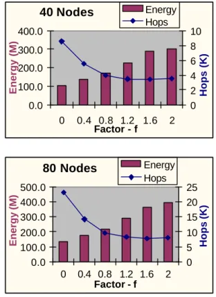
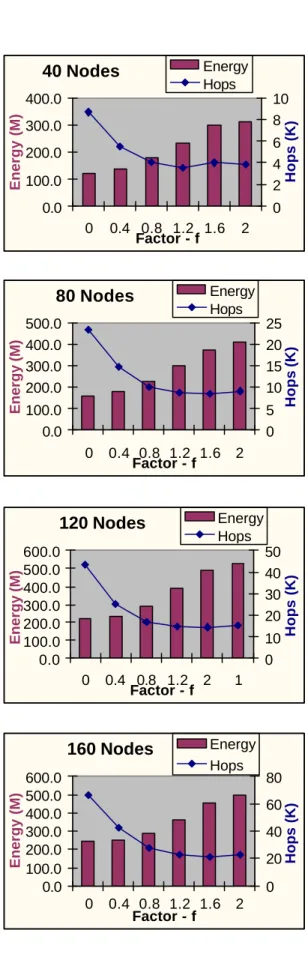
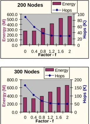
(11) different numbers of evenly distributed nodes on the 800m × 800m region. By inspecting this figure and constructing connectivity graphs, we obtained Rscg. Table 5.3.1 Rscg values (Area = 800m × 800m) Node Number 20 40 60 80 100 120. values listed in Table 5.3.1. Figure 5.3.1-2 indicates that Rscg is inversely proportional to the square-root of the network density.. 1.2 1.0 0.8. 60 80. 0.6. 100 120. 0.4. 140 160. 0.2. 180 200. 130 110 110 100 83.5. 38 0. 34 0. 26 0 30 0. 22 0. 18 0. 0.0 60 10 0 14 0. Rscg (m). 5.3.2 f × R scg vs. Delivery Energy and Latency In Section 4, we designed an approach to locate the optimal transmission distance that could bridge the delivery energy and latency. Figure 5.3.2-1(for static network) and 5.3.2-2 (for mobile network) reveal the relationship between these two metrics and the transmission radius.. 20 40. 20. 380 240 190 170 170 150. Node Number 140 160 180 200 300. Node Number. Physical Connectivity. Radius. 40 Nodes. Energy Hops 10 8 6 4 2 0. Energy (M). 400.0. Hops (K). 300.0 200.0 100.0 0.0 0. 0.4 0.8 1.2 1.6 Factor - f. 80 Nodes. 1 density. 10. Energy Hops. 500.0 400.0 300.0. 25 20 15. 200.0 100.0 0.0. 10 5 0 0. Figure 5.3.1-2 Rscg vs.. 2. 0.4 0.8 1.2 1.6 Factor - f. 2. Hops (K). Figure 5.3.1-1 Connectivity vs. Radio Range. Energy (M). Connectivity. Rscg (m).

(12) 0. Energy (M). Hops (K). Energy Hops. 200. 400.0. 100. 200.0. 50 0. 600.0 500.0 400.0 300.0 200.0 100.0 0.0. Figure 5.3.2-1 Static Mode – Speed: 0. 11. Hops (K). Energy Hops. 10 0 0.4 0.8 1.2 2 Factor - f. 1. Energy Hops. 80 60 40 20 0. 0. 2. 2. 50 40 30 20. 160 Nodes 150. 0.0. 0.4 0.8 1.2 1.6 Factor - f. 600.0 500.0 400.0 300.0 200.0 100.0 0.0 0. 600.0. 0 0.4 0.8 1.2 1.6 Factor - f. 5 0. 2. Energy (M). 300 Nodes. 100.0 0.0. 120 Nodes 100 80 60 40 20 0. 0.4 0.8 1.2 1.6 Factor - f. Energy Hops 25 20 15 10. 0. Energy Hops. 2. 500.0 400.0 300.0 200.0. 2. 600.0 500.0 400.0 300.0 200.0 100.0 0.0. 0.4 0.8 1.2 1.6 Factor - f. Hops (K). Energy (M). 80. 20. 0. 0. 80 Nodes. 40. 200 Nodes Energy (M). Energy Hops. 0.4 0.8 1.2 1.6 Factor - f. 0.0 0. 60. 0. 100.0. 6 4 2. 200.0. 2. Hops (K). Energy (M). 600.0 500.0 400.0 300.0 200.0 100.0 0.0. 300.0. 0.4 0.8 1.2 1.6 Factor - f. Hops (K). 0 0.4 0.8 1.2 1.6 Factor - f. 10 8. 2. Hops (K). 20 10. Energy Hops. 400.0 Energy (M). 30. 160 Noedes. Energy (M). 50 40. 0. 800.0. 40 Nodes Hops (K). 600.0 500.0 400.0 300.0 200.0 100.0 0.0. Energy Hops. Hops (K). Energy (M). 120 Nodes.

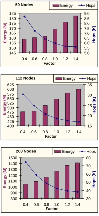
(13) Most simulation parameters used in this section are consistent with GPSR. The value of Rscg is set at 210m from calculation and experimental observations; the beacon range is set at 250m to hold the beaconing energy at the same level as GPSR. Measurements in experiment (Figure 5.4-1) show the energy-efficiency has been achieved by MGPSR. However, it is worthy noticing that because the vertical dimension (300, 450, and 600m) of the region is not much longer than the 250m radio range, very few voids could exist. That means, perimeter mode is rarely entered. The advantage of Delaunay-based graph in reducing nodal delays becomes insignificant, which probably accounts for the longer transmission latency.. Hops (K). 100 80 60 40 20 0 0.4 0.8 1.2 1.6 Factor - f. 300 Nodes. 2. Energy Hops. 800.0. 200. 600.0. 150. 400.0. 100. 200.0. 50. 0.0. Hops (K). Energy (M). 600.0 500.0 400.0 300.0 200.0 100.0 0.0 0. Energy (M). 5.4 MGPSR vs. GPSR. Energy Hops. 200 Nodes. Curves in Figure 5.4-2 and 5.4-3 reveal the relationship between energy/hop number and the factor value , which exhibits similar properties as previous ones.. 0 0 0.4 0.8 1.2 1.6 Factor - f. 2. Figure 5.3.2-2 Mobile Mode – Speed: 50-60 As expected, the energy consumption rises with ascending packet transmission radius. The shorter the distance between each pair of sender and receiver, the lower the energy cost. In contrast, the downward sloped curve of hop numbers suggests that the routing time decrements fast with increasing factor, especially at small values. The existentially optimal balancing point is within the range of 0 .6 − 0 .8 Rscg. Energy (Pause=0). GPSR. MGPSR. Energy (M). 1600. 81.44%. 1400 1200 1000 800. 83.69%. 600 400. 92.87%. 200. where the two asymptotes meet.. 0 50. 112. 200. Nodes. One reasonable inference is that forwarding packets to neighbors at a distance of 0.6 − 0.8Rscg usually can alleviate the energy wastage with little increment in routing delay. Another noticeable fact is that a value slightly larger than 0.6 − 0. 8Rscg could be set as the upper bound of the beacon range. Furthermore, this range is closely related to the network density via Rscg . Consequently, the transmission range can be. GPSR. Energy (M). Energy (Pause=30). preset on mobile devices when the network density can be estimated in advance. Or, by analyzing the changing environment, nodes may automatically regulate the transmission range correspondently.. MGPSR. 1600 1400. 81.14%. 1200 1000 800. 84.07%. 600. 88.31%. 400 200 0 50. 112. Nodes. 12. 200.

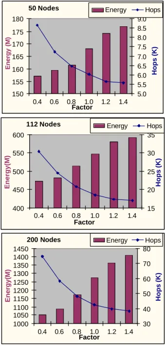
(14) MGPSR. 50 Nodes. Energy. Hops 9.0 8.5 8.0 7.5 7.0 6.5 6.0 5.5 5.0. 180 175. 1200 1000 800. 84.42%. 600 400. 170. Hops (K). 81.58%. 1400. 165 160 155. 88.00%. 200. 150. 0 50. 112. 0.4. 200. 0.6. Nodes Hops (Pause=0). GPSR. 112 Nodes. Energy(M). 118.85%. 50. Hops (K). MGPSR. 40 30. 115.78% 20. 127.09%. 10. 50. 1.4. 600. Hops 35. 550. 30. 500. 25. 450. 20. 112. Energy. 15 0.4. 200. 0.6. Nodes GPSR. Hops (Pause=30). MGPSR. Energy(M). 119.81%. 50. Hops (K). 1.2. 400. 0. 40 30. 115.93% 20. 107.64%. 10 0 50. 112. 200. Nodes GPSR. Hops (Pause=60). MGPSR. 45 40 35 30 25. 117.31%. 20 15 10 5 0. 111.04%. 50. 112. 200 Nodes 1450 1400 1350 1300 1250 1200 1150 1100 1050 1000 0.4 0.6. 0.8 1.0 Factor. 1.2. 1.4. Energy. Hops 80 70 60 50 40 30. 0.8 1.0 Factor. 1.2. 1.4. Figure 5.4-2 MGPSR (Pause Time = 0 ). 119.49%. 50. Hops (K). 0.8 1.0 Factor. 200. Nodes. Figure 5.4-1 GPSR vs. MGPSR (Factor = 0.7) 13. Hops (K). Energy (M). Energy (M). 1600. Hops (K). GPSR. Energy (Pause=60).

(15) 185 180 175 170 165 160 155 150 145. 9.0 8.5 8.0 7.5 7.0 6.5 6.0 5.5 5.0 0.4. 0.6. 0.8 1.0 Factor. 1.4. Energy. Hops. 625 600 575 550 525 500 475 450 425 400. 35 30 25. We devised an empirical strategy for energy-latency efficient route selection. Intensive simulations demonstrated that the proposed density-based forwarding algorithm could minimize the amount of energy with little performance degradation in terms of delivery time. Severe constraint on battery resources heightened the need for such a powerefficient routing strategy. The idea behind this solution could be adopted in various routing protocols besides MGPSR.. 20 15 0.4. 0.6. 0.8 1.0 Factor. 200 Nodes. Energy (M). In addition, the findings confirm that 1+- GLDD leads to considerably higher connectivity and, as such, it supports more efficient and robust routing. This higher connectivity comes at minimal additional cost. In fact, because of the planarity of the graph, the overall space required to maintain the graph on all nodes can be bounded by a linear function of the number of neighboring nodes. The time complexity for the construction and maintenance of the graph is also well within an acceptable bound. The instant response to link-state changes fits it well in mobile networks.. Hops (K). Energy (M). 112 Nodes. 1.2. MGPSR in balancing energy consumption and delivery time.. Hops. Hops (K). Energy. 1.2. 1.4. Energy. Hops. 1500 1400 1300. 80. 1200 1100. 60. In short, MGPSR overcomes the present limitations of GPSR as well as widens its scope. It has been theatrically and empirically proved to be quite promising in the territory of mobile ad hoc networks. Future research is required to address the problem how nodes could automatically adjust the greedy forwarding radius in non-uniformly distributed networks.. 70. 50. 1000 900 800. Hops (K). Energy (M). 50 Nodes. 40 30 0.4. 0.6. 0.8 1.0 Factor. 1.2. 1.4. REFERENCE [1] ADRIAN, B. Computing Dirichlet Tessellations. Computer Journal 24(2): 162– 166, 1981.. Figure 5.4-3 MGPSR (Pause Time = 30 ). 6.. [2] BASAGNI, S., CHLAMTAC, I., SYROTIUK, V., AND WOODWARD, B. A Distance Routing Effect Algorithm for Mobility (DREAM). In Processing of the Fourth Annual ACM/IEEE International Conference on Mobile Computing and Networking (MOBICOM ’98), October 1998.. CONCLUSION. We have presented a new ad hoc network routing protocol, the Modified Greedy Perimeter Stateless Routing (MGPSR) protocol. We have also compared this scheme with the original GPSR protocol on quite a number of networks with uniform distribution and simulation results quantitatively verified the merits of 14.

(16) [3] BLELLOCH, G. E., MILLER, G. L., TALMOR, D. Developing a Practical Projection-Based Parallel Delaunay Algorithm. In Proceeding of ACM Symposium on Computational Geometry, 1996.. [13] EPPSTEIN, D. Spanning Trees and Spanners. In J.-R. Sack and J. Urrutia, editors, Handbook of Computational Geometry, pages 425-461. Elsevier Science Pbulishers B.C. NorthHolland, Amsterdam, 2000.. [4] BROCH, J., MALTZ, D., JOHNSON, D., HU, Y., AND JETCHEVA, J. A Performance Comparison of Multi-hop Wireless Ad Hoc Network Routing Protocols. In Proceedings of the Fourth Annual ACM/IEEE International Conference on Mobile Computing and Networking (MOBICOM ’98), August 1998.. [14] FORTUNE, S. Sweepline Algorithms for Voronoi diagrams. Algorithmica 2: 153-174, 1987. [15] GAO, J., GUIBAS, L. J., HERSHBERGER, J., Zhang, L., AND ZHU, A. Geometric Spanner for Routing in Mobile Networks. In proceeding of MobiHoc, 2001.. [5] BROCH, J., MALTZ, D., AND JOHNSON, D. The Dynamic Source Routing Protocol for Mobile Ad Hoc Networks. In Proceeding of the Fourth Annually ACM/IEEE International Conference on Mobile computing and Networking (MOBICOM ’98), October 1998.. [16] GARBIEL, K., AND SOKAL, R. A New Statistical Approach to Geographic Variation Analysis. Systematic Zoology 18: 259-278, 1969. [17] GARCIA-LUNA-ACEVES, J., SPOHN, M. AND BEYER, D. Source Tree Adaptive Routing (STAR) Protocol (Internet-Draft). Mobile Ad hoc Network (MANET) Working Group, IETF, October 1999.. [6] CAPKUN, S., HAMDI, M., HUBAUX, J. Gpsfree Positioning in Mobile Ad-hoc Networks. In proceeding of Hawaii Int. Conf. on System Science, January 2001.. [18] HAAS, Z., AND PEARLMAN, M. The Zone Routing Protocol for Highly Reconfigurable Ad Hoc Networks. In Proceedings of the SIGCOMM ’98 Conference on Communications Architectures, Protocols and Applications, September 1998.. [7] Cignoni, P., Montani, C., Perego, R., AND Scopigno, R. Parallel 3D Delaunay Triangulation. Eurographics 93: 129-142, 1993. [8] CHARLES, L. L. Software for C- Surface Interpolation. Mathematical Software III (John R. R, editor): 161–194. Academic Press, New York, 1977.. [19] HARDWICK, J. C. Implementation and Evaluation of an Efficient 2D Parallel Delaunay Triangulation Algorithm. In proceeding of ACM symposium of Parallel Algorithms and Architectures, 1997.. [9] CHENG, C., RILEY, R., KUMAR, S., AND GARCIAL-LUNA-ACEVES, J. A Loop-free Bellman-Ford Routing Protocol without Bouncing effect. In ACM SIGCOMM ’89, September 1989.. [20] IEEE COMPUTER SOCIETY LAN MAN STANDARDS COMMITTEE. Wireless LAN Medium Access Control (MAC) and Physical Layer (PHY) Specifications. IEEE Std. 802.111997, 1997.. [10] CHIANG, C. Routing in Clustered Multihop, Mobile Wireless Networks with Fading Channel. In Proceedings of IEEE SICON ’97, April 1997.. [21] JAQUET, P., MUHLETHALER, P., AND QAYYUM, A. Optimized Link State Routing Protocol. Internet Draft (work in progress), August 1998.. [11] DAVIDd, F. W. Computing the n-dimensional Delaunay Tessellation with Application to Voronoi Polytopes. Computer Journal 24(2):167–172, 1981.. [22] JEFFREY HIGHTOWER AND GAETANO BORRIELLO. Location Systems for Ubiquitous Computing. Computer, 34(8):57-66, August 2001.. [12] DENIS, C. Delaunay Triangulation Java Program. http://cage.rug.ac.be/~dc/alhtml/ Delaunay. Html.. 15.

(17) [23] KAHN, M., KATZ, R., AND PISTER, K. Mobile Networking for Smart Dust. In Proceedings of the Fifth Annual ACM/IEEE International Conference on Mobile Computing and Networking (MOBICOM ’99), August 1999.. the Conference on Computer Communications (IEEE INFOCOM ’97), April 1997. [31] PARK, V., AND CORSON, M. A Performance Comparison of the Temporally-Ordered Routing Algorithm and Ideal Link-State Routing. In Proceedings of IEEE International Symposium on Systems and Communications. IEEE Computer Society Press, June 1998.. [24] KARP, B AND KUNG, H. Geographic Routing for Wireless Networks, In Proceedings of the ACM/IEEE International Conference on Mobile Computer and Networking (MOBICOM), 2000.. [32] PERKINS, C., AND BHAGWAT, P. Highly Dynamic Destination Sequenced DistanceVector Routing (DSDV) for Mobile Computers. ACM SIGCOMM ’94 Computer Communications Review 24(4):234-244, October 1994.. [25] KO, Y., AND VAIDYA, N. Location-Aided Routing in Mobile Ad Hoc Networks. In Proceedings of the Fourth Annual ACM/IEEE International Conference on Mobile Computing and Networking (MOBICOM ’98), August 1998.. [33] PERKINS, C., AND ROYER, E. Ad-hoc OnDemand Distance Vector Routing. In Proceedings of the Second Annual IEEE Workshop on Mobile Computing Systems and Applications , February 1999.. [26] KO, Y., AND VAIDYA, N. GeoTORA: A Protocol for Geocasting in Mobile Ad Hoc Networks. March 2000.. [34] PERKINS, C. Ad Hoc Networking. Addison Wesley, 2000.. [27] LI, J., JANNOTTI, J., DE COUTO, D., KARGER, D., AND MORRIS, R. A Scalable Location Service for Geographic Ad-Hoc Routing. In Proceedings of the Sixth Annual ACM/IEEE International Conference on Mobile Computing and Networking (MOBICOM 2000) , August 2000.. [35] PREPARATA, F. P. Computational geometry: an introduction. New York: Springer-Verlag, 1985. [36]SIBSON, R. Locally equiangular triangulations. The Computer Journal Vol.2 (3): 243-245, 1973.. [28] LUAN, L. AND HSU, W. J. Localized Delaunay Triangulation for Topological Construction and Routing on MANETs. Technical Report: CAIS-TR-02-46, Centre for Advanced Information Systems, School of Computer Engineering, Nanyang Technological University, Singapore, July 2002. Available from: http://www.cais.ntu.edu.sg:8000/Research_Pro jects/Technical_Reports/technical_reports.html.. [37]SIDHU, D., FU, T., ABDALLAH, S., NAIR, R. AND COLTUN, R. Open Shortest Path First (OSPF) Routing Protocol Simulation. In Proceed ings of ACM SIGCOMM '93, 1993. [38] SINGH, S., WOO, M., AND RAGHAVENDRA, C. Power-Aware Routing in Mobile Ad Hoc Networks. In The Fourth Annual ACM/IEEE International Conference on Mobile Computing and Networking, 1998.. [29] MALTZ, D., BROCH, J., JETCHEVA, J., AND JOHNSON, D. The Effects of OnDemand Behavior in Routing Protocols for Multihop Wireless Ad Hoc Networks. IEEE Journal on Selected Areas in Communications 17, 8, August 1999.. [39] SIVAKUMAR, R. AND BHARGHAVAN, V. Spine Routing in Ad Hoc Networks. http://uiuc.edu/Papers/ccj98.ps.gz 1998. [40] SIVAKUMAR, R., SINHA, P., AND BHARGHAVAN, V. CEDAR: Core Extraction Distributed Ad Hoc Routing Algorithm. In Proceedings of IEEE INFOCOM ’97, April 1997.. [30] PARK, V., AND CORSON, M. A Highly Adaptive Distributed Routing Algorithm for Mobile Wireless Networks. In Proceedings of. 16.

(18) [41] TAKAGI, G. AND KLEINROCK, L. Optional Transmission Ranges For Randomly Distributed packet Radio Terminals. IEEE Trans. Communications, 32(3):246-257, March 1984.. d ( m, z ) <. 1 d ( x, y) , where m denotes the mid-point of 2. xy .. In Figure A-2, C(1,3), the shaded circle with diameter 13 must be void of nodes so that edge 13 could be in GG.. [42] TOUSSAINT, G. The Relative Neighborhood Graph of a Finite Planar Set. Pattern Recognition 12, 4: 261-268, 1980. [43] TSUCHIYA, P. The Landmark Hierarchy: A New Hierarchy for Routing in Very Large Networks. IEEE SIGCOMM 88, September 1988. [44] XU, Y., HEIDEMANN, J., AND ESTRIN, D. Geography-informed Energy Conservation for Ad Hoc Routing. In Proceedings of the Seventh Annual ACM/IEEE International Conference on Mobile Computing and Networking (ACM MOBICOM), July 2001.. Figure A-2 The GG Graph 13 is not in GG due to the existence of node 2.. Appendix A. The void area required in an RNG contains the circular region in GG, so GG is superset of RNG, which is illustrated in Figures 5.2.2-1, 5.2.2-2, 5.2.2-4, and 5.2.2-5.. Relative Neighborhood Graph (RNG). Delaunay Triangulation. Definition Given two (arbitrary) nodes x and y, the edge xy is in RNG if and only if the distance between vertices x and y is less than or equal to the distance between any other vertex z, and whichever of x and y is farther from z. In other words, for any vertex z other than x and y, if d ( x, y) ≤ max[ d ( x, z ), d ( y, z )] , xy is an RNG edge. (Figure A-1). Definition Any circle in the plane is said to be empty if it encloses no vertex of a given set of vertices V (vertices are permitted on the circle). The circumcircle of a triangle is the unique circle that passes through all three of its vertices. A triangle is said to be Delaunay if and only if its circumcircle is empty. Definition Let u and v be any two vertices in V. A circumcircle (circumscribing circle) of the edge uv is any circle that passes through u and v. The edge uv is in Global DT if and only if there exists an empty circumcircle of uv . (Figure A-3). Figure A-1 The RNG Graph is in RNG, if and only if the shaded lunar area, intersection of the two inner circles, is empty of any (witness) node 2. 13. Gabriel Graph (GG) Definition Given two arbitrary nodes x and y, an edge xy is in GG if there exists no other vertex z such that. Figure A-3 Global Delaunay Triangulation 17.

(19)