A Multivariate Long Memory Model for the Specification of Real Output in the US, the UK, and Canada

全文

(1)International Journal of Business and Economics, 2007, Vol. 6, No. 2, 135-146. A Multivariate Long Memory Model for the Specification of Real Output in the US, the UK, and Canada Luis A. Gil-Alana* Faculty of Economics, University of Navarra, Spain. Abstract This paper deals with a multivariate long memory model for the specification of real output in the US, the UK, and Canada. We examine the orders of integration of the three time series first individually and then allow cross dependence between observations. Performing univariate analysis, results show that the three series have orders of integration higher than 1, especially Canada. The multivariate model supports this view, finding conclusive evidence of non-stationarity for the three series and higher orders of integration for Canada than for the UK or the US. With respect to the cross-dependence structure, it seems that the US and Canada, and the US with the UK present the highest degrees of correlation across countries. Key words: multivariate tests; fractional integration; long memory JEL classification: C22. 1. Introduction Long memory models have become in recent years alternative credible ways of modeling many macroeconomic time series. Tests for fractional integration have been examined by Robinson (1991, 1994), Sowell (1992), Agiakloglou and Newbold (1994), and Tanaka (1999) among others, all in a univariate framework. With no multivariate tests available for testing the order of integration of the series, research interested in multiple time series have been forced to apply univariate tests to each element of the multiple time series. This paper uses an extension of the univariate tests of Robinson (1994) to the multivariate case, and we examine the degrees of integration of real output in the US, the UK, and Canada first in a univariate context and then in a multivariate system. In the latter case, we are able to capture a much richer dynamic behavior than the univariate work, incorporating the potential correlation across the series. Since many time series of interest are likely to Received June 17, 2005, revised August 20, 2007, accepted August 30, 2007. * Correspondence to: University of Navarra, Faculty of Economics, Edificio Biblioteca, Entrada Este, E31080 Pamplona, Spain. E-mail: alana@unav.es. Comments of an anonymous referee are gratefully acknowledged. The author also acknowledges financial support from the Ministerio de Ciencia y Tecnologia (SEJ2005-07657, Spain)..

(2) 136. International Journal of Business and Economics. be influenced by the same set of events, it is straightforward to consider Lagrange Multiplier (LM) tests in a multivariate framework by also modeling the covariation of the series. Section 2 briefly describes the univariate procedure. Section 3 extends the tests to the multivariate case. Section 4 contains the empirical application, while Section 5 contains concluding comments. 2. The Univariate Tests of Robinson (1994) We define an I ( 0 ) process {ut , t = 0, ± 1, K} as a covariance stationary process with spectral density function that is positive and finite at the zero frequency. In this context, we say that {xt , t = 0, ± 1, K} is I ( d ) if: (1 − L) d xt = ut for t = 1, 2,K , xt = 0 for t ≤ 0 .. (1) (2). If d = 0 in (1), xt = ut , and we say that xt is “short memory” as opposed to the concept of “long memory” in case of d > 0 . The fractional differencing parameter d plays a crucial role from both statistical and economic viewpoints. Thus, for example, if d ∈ (0, 0.5) , xt is covariance stationary, and if d ∈ [0.5, 1) , xt is no longer stationary but is still mean reverting, with the effect that shocks die away in the long run. Finally, if d ≥ 1 , the series is non-stationary and non-mean-reverting. This result has strong implications in terms of economic policy. Thus, for example, if a time series is mean-reverting (i.e., d < 1 ), there is less need for policy action than in the case of a unit root, since the series will return to its path sometime in the future. On the other hand, if the series is I (1) , strong policy actions will be required to bring the variable back to its level since the effect of the shocks will persist forever. It thus appears crucial to examine the order of integration of the series in order to determine the persistence of the shocks. We first describe the univariate tests of Robinson (1994). He considers the regression model: yt = β ' zt + xt , t = 1, 2,K ,. (3). where yt is the time series we observe, β is a k × 1 vector of unknown parameters, z t is a k × 1 vector of deterministic regressors, and xt is given by (1). Robinson (1994) proposed an LM test of the null hypothesis: H 0 : d = d0. (4). in (1)–(3) for any real value d 0 . The functional form of the test statistic (denoted Rˆ ) is fully described in Robinson (1994). Based on the null hypothesis H 0 , he established that under certain regularity conditions:.

(3) Luis A. Gil-Alana Rˆ →d χ12 as T → ∞ .. 137 (5). This version of the test permits us to test unit roots in the classical sense (e.g., Dickey and Fuller, 1979; Phillips and Perron, 1988; Kwiatkowski et al., 1992) in the case of d 0 = 1 in (4). However, unlike these previous procedures, Robinson’s (1994) method has several distinguishing features. First, the asymptotic null distribution is standard, in the sense that we do not need to rely on critical values obtained via Monte Carlo simulations. Also, the tests are efficient in the Pitman sense, and these two properties hold independent of the inclusion or exclusion of deterministic regressors and of the different ways of modeling the I (0) disturbances, which is another unusual feature in most unit root tests, with the limiting distribution changing with features of the regressors. 3. A Multivariate Fractional Test Suppose that yt = ( y1t ,K , yNt )′ is the N × 1 time series vector we observe and that it is driven by the following model: ⎛ (1 − L) d1 ⎜ ⎜ M ⎜ 0 ⎝. 0 L O M L (1 − L) d N. ⎞ ⎛ y1t ⎞ ⎛ u1t ⎞ ⎟⎜ ⎟ ⎜ ⎟ ⎟ ⎜ M ⎟ = ⎜ M ⎟ , t = 1, 2,K , ⎟⎜ y ⎟ ⎜u ⎟ ⎠ ⎝ Nt ⎠ ⎝ Nt ⎠. (6). where ut = (u1t ,K , u Nt )′ is an I (0) vector process with spectral density matrix F (λ ) that is positive definite. Thus, it may be a white noise vector process but it may also include, for example, a VAR structure. As in Robinson (1994), we could also have included an intercept and/or a linear time trend. However, in order to simplify the computation of the test statistic, we prefer to work directly with the original series, subtracting the sample mean before performing the analysis in the empirical application in Section 4. Similar to the univariate tests of Robinson (1994), we test the null hypothesis: H 0 : d ≡ (d1 ,K , d N )′ = (d10 ,K , d N 0 )′ ≡ d 0. (7). in (6) for real values d 0 . Let us suppose that ut in (6) is a vector process generated by a parametric model of form: ∞. ut = ∑ A( j;τ ) ε t − j , t = 1, 2,K ,. (8). j =0. where ε t is white noise and K is the unknown variance-covariance matrix of ε t . The spectral density matrix of u t in (8) is:.

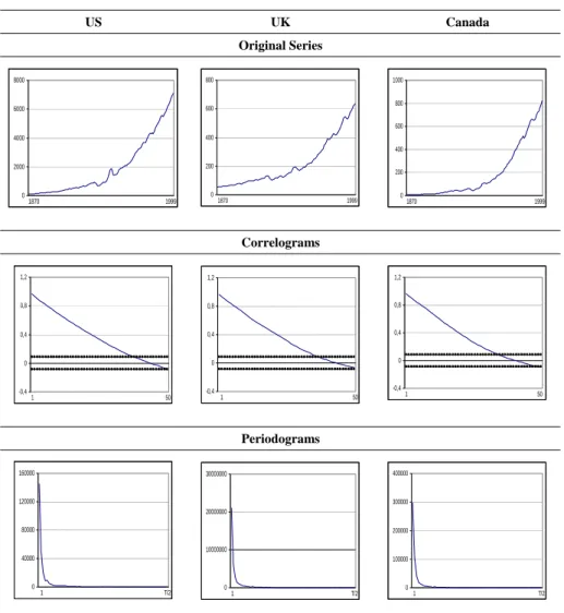
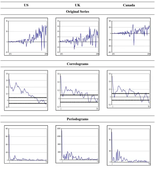
(4) 138. International Journal of Business and Economics f (λ ;τ ) =. 1 k (λ ;τ ) Kk (λ ;τ )* , 2π. (9). where k (λ ;τ ) = ∑ j = 0 A( j;τ ) e i λ j and k * means the complex conjugate transpose of k . A number of conditions are required on A and f when deriving the test statistic; their practical implications being that though ut is capable of exhibiting a much stronger degree of autocorrelation than a multiple ARMA process, its spectral density matrix must be finite, with eigenvalues bounded and bounded away from zero. In Gil-Alana (2003a, b), it is shown that a LM test S% of H 0 in (6) satisfies: ∞. S% →d χ N2 as T → ∞ .. (10). Thus, the limiting distribution is standard, unlike what happens in other procedures for testing unit roots in univariate models, based on autoregressive (AR) alternatives. In fact, it is the fractional characteristic of the model and its smoothness around the unit root case that makes the distribution standard for all real values d 0 . Results based on Monte Carlo experiments on these multivariate tests were carried out in Gil-Alana (2003a), and it was shown that the tests perform relatively well in finite samples against fractional-type alternatives. 4. An Empirical Application The time series data analyzed in this section corresponds to annual US, UK, and Canadian real output for the time period 1870–1999, obtained from the International Monetary Fund database. Figure 1 displays the original series along with their corresponding correlograms and periodograms. All series have a non-stationary appearance, which is corroborated by the correlograms with values decaying very slowly, and also by the periodograms with a large peak around the smallest frequency. Figure 2 displays similar plots based on the first differenced data. We see that the correlograms still present significant values even at some lags relatively away from 0 and similarly the periodograms still show peaks at the zero frequency, suggesting that a component of long memory is still present in the first differenced data. We start by performing the univariate tests of Robinson (1994). We compute the test statistic rˆ = Rˆ , testing H 0 in model (1) and (3), assuming that the disturbances are white noise and weakly autocorrelated. In the latter case, we consider AR models and Bloomfield’s (1973) exponential spectral model, denoted B( k ) for the k th-order model. This is a non-parametric approach to modeling the I (0) disturbances, which produce autocorrelations decaying exponentially as in the AR case..

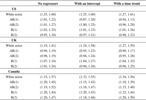
(5) Luis A. Gil-Alana. 139. Figure 1. Original Time Series with Corresponding Correlograms and Periodograms US. UK. Canada. Original Series 8000. 800. 6000. 600. 4000. 400. 2000. 200. 1000 800 600 400. 0. 0. 1870. 1999. 200. 1870. 1999. 0. 1870. 1999. Correlograms 1,2. 1,2. 1,2. 0,8. 0,8. 0,8. 0,4. 0,4. 0,4. 0. 0. 0. -0,4. 1. 50. -0,4. -0,4. 1. 50. 1. 50. Periodograms 160000. 400000. 30000000. 120000. 300000. 20000000 80000. 200000. 10000000 40000. 0. 100000. 1. T/2. 0. 1. T/2. 0. 1. T/2. Notes: In the correlograms, the large sample standard error under the null hypothesis of no autocorrelation is 1 T or roughly 0.08.. Table 1 displays the 95% confidence intervals of those values of d 0 where H 0 cannot be rejected. We take (1) and (3) with zt = (1, t )′ , t ≥ 1 , and (0, 0)′ otherwise. Thus, under H 0 , the model becomes: yt = β1 + β 2 t + xt , t = 1, 2,K ,. (11). (1 − L) xt = ut , t = 1, 2,K .. (12). do. We examine the cases of white noise, AR( k ), and B( k ), k = 1, 2 , disturbances. First, we concentrate on the case of β1 = β 2 = 0 a priori (i.e., we do not consider.

(6) International Journal of Business and Economics. 140. regressors in the undifferenced model (11)). Then we study the cases of β1 unknown and β 2 = 0 a priori (i.e., with an intercept), and finally both β1 and β 2 unknown (i.e., with an intercept and a linear time trend). Figure 2. First Differenced Time Series with Corresponding Correlograms and Periodograms US. UK. Canada. Original Series 40. 400. 40 30. 20. 200. 20 0 10 -200. 0. 0 -400. -10 -20. 1871. 1999. -20. 1871. 1999. -600. 1871. 1999. Correlograms 0,8 0,6. 0,6. 0,6. 0,4. 0,4. 0,2. 0,2. 0,4 0,2. 0. 0. 0. -0,2. -0,2. -0,2. 1. 1. 50. 50. Periodograms 400. 16000. 300. 12000. 200. 8000. 100. 4000. 120. 80. 0. 0. 1. T/2. 40. 1. T/2. 0. 1. T/2. Notes: In the correlograms, the large sample standard error under the null hypothesis of no autocorrelation is 1 T or roughly 0.08.. Starting with the results for the US, we observe that if we do not include regressors, the unit root null hypothesis is rejected for all types of disturbances except if they are B(2). The values of d 0 where H 0 cannot be rejected range between 0.95 (when ut is B(2)) and 1.60 (when ut is white noise). Similar results are obtained in case of including an intercept and/or a linear time trend, though the.

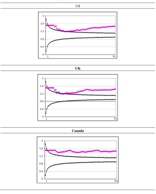
(7) Luis A. Gil-Alana. 141. unit root is not rejected here if the disturbances are AR(1). Similarly for the UK, if u t is white noise, the unit root is decisively rejected in favor of higher orders of integration, the values ranging from 1.19 (with no regressors) to 1.59 (with a linear time trend). If the disturbances are autocorrelated, the unit root is also rejected when u t is AR(1), while it is not for the remaining types of disturbances. Finally, the results for Canada are definitely less ambiguous, and the unit root is rejected for all types of disturbances and all types of regressors. The values of d 0 where H 0 cannot be rejected oscillate now from 1.10 (when u t is AR(1) with a linear trend) to 1.57 (when ut is white noise with no regressors). Table 1. Confidence Intervals of the Non-Rejection Values of No regressors. With an intercept. d0. With a time trend. US. White noise. (1.25, 1.60). (1.25, 1.60). (1.27, 1.61). AR(1) AR(2). (1.01, 1.22) (1.01, 1.27). (0.87, 1.20) (1.00, 1.25). (0.94, 1.13) (0.96, 1.28). B(1) B(2). (1.02, 1.25) (0.95, 1.18). (1.01, 1.23) (0.97, 1.21). (1.01, 1.26) (0.98, 1.23). UK. White noise. (1.19, 1.41). (1.24, 1.58). (1.27, 1.59). AR(1) AR(2). (0.96, 1.19) (0.98, 1.19). (0.95, 1.23) (0.96, 1.24). (0.90, 1.17) (0.95, 1.28). B(1) B(2). (1.07, 1.34) (1.01, 1.24). (1.04, 1.27) (0.96, 1.26). (1.04, 1.32) (0.96, 1.25). Canada. White noise. (1.33, 1.57). (1.32, 1.55). (1.34, 1.56). AR(1) AR(2) B(1) B(2). (1.20, 1.45) (1.19, 1.52) (1.20, 1.44) (1.20, 1.47). (1.15, 1.42) (1.16, 1.47) (1.20, 1.43) (1.18, 1.46). (1.10, 1.39) (1.15, 1.48) (1.22, 1.44) (1.20, 1.50). The results in Table 1 vary substantially depending on how we specify the I (0) disturbances. Because of this, we have also performed a semiparametric procedure (Robinson, 1995), which is robust to the different types of disturbances. It is a local “Whittle estimate” in the frequency domain, considering a band of frequencies that degenerates to zero. Robinson (1995) proved that: m (dˆ − d o ) → d N (0,1/ 4) as T → ∞ ,. where d 0 is the true value of d and with the only additional requirement that m → ∞ slower than T ..

(8) 142. International Journal of Business and Economics Figure 3. Estimates of. d 0 based on Robinson (1995) and the Unit Root Intervals US. 2 1,6 1,2 0,8 0,4 0. 1. T/2. UK 2 1,6 1,2 0,8 0,4 0. 1. T/2. Canada 2 1,6 1,2 0,8 0,4 0. 1. T/2. Figure 3 presents the results based on Robinson (1995) for a range of values of m from 1 to T 2 . Because of the non-stationary nature of the series, the analysis is based on the first differenced data, then adding 1 to the estimated values to obtain the proper values of d . We also display 95% confidence intervals corresponding to the unit root case. We see that for the three series, practically all the estimates are above the unit root interval. Moreover, for the US and the UK, the values oscillate between 1.2 and 1.5, and they are slightly higher for Canada..

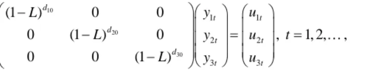
(9) Luis A. Gil-Alana. 143. Next, we perform the multivariate analysis and compute the test statistic described in Section 3, testing the null hypothesis (7) in (6), assuming first that u t is white noise. Thus, under this H 0 , the model becomes: ⎛ (1 − L) d10 ⎜ 0 ⎜ ⎜ 0 ⎝. 0 (1 − L) 0. 0 d 20. 0 (1 − L). d30. ⎞ ⎛ y1t ⎞ ⎛ u1t ⎞ ⎟⎜ ⎟ ⎜ ⎟ ⎟ ⎜ y2t ⎟ = ⎜ u2t ⎟ , t = 1, 2,K , ⎟⎜ y ⎟ ⎜u ⎟ ⎠ ⎝ 3t ⎠ ⎝ 3t ⎠. (13). where d10 , d 20 , and d30 are the orders of integration of the US, the UK, and Canada. We calculate the statistic for values d10 , d 20 , and d30 between 0 and 2.5 in increments of 0.25. However, instead of reporting the values for all statistics, we report in Table 2 only those ( d10 , d 20 , d30 ) combinations where H 0 cannot be rejected at the 5% level. The first thing we observe is that the null hypothesis of three unit roots (i.e., d10 = d 20 = d30 = 1 ) is rejected, and all non-rejection values are for values of d10 , d 20 , and d30 at least 1, implying non-mean-reverting behavior. Moreover, we observe that the values of d30 are nearly always higher than d10 and d 20 , implying a stronger degree of integration for Canada than for the UK and the US in spite of the cross-covariance dependence permitted between the series. Table 2. Values of d where H 0 Cannot Be Rejected at the 5% Level: White Noise Disturbances d10. d 20. d 30. Test Statistic. 1.00. 1.50. 1.75. 4.065. 1.00 1.00. 1.50 1.75. 2.00 1.50. 2.460 5.609. 1.00 1.00 1.00 1.00 1.00 1.25 1.25 1.25 1.25 1.25 1.50 1.50 1.50 1.75 1.75 1.75 2.00 2.00 2.00. 1.75 1.75 2.00 2.00 2.00 1.25 1.25 1.25 1.50 1.75 1.00 1.00 1.25 1.00 1.00 1.00 1.00 1.00 1.00. 1.75 2.00 1.50 1.75 2.00 1.50 1.75 2.00 1.50 1.50 1.75 2.00 1.50 1.50 1.75 2.00 1.50 1.75 2.00. 1.025 0.228 3.986 0.351 0.00001 0.229 0.278 0.681 2.772 6.083 3.171 1.957 3.654 3.545 0.003 0.361 1.003 0.531 0.286.

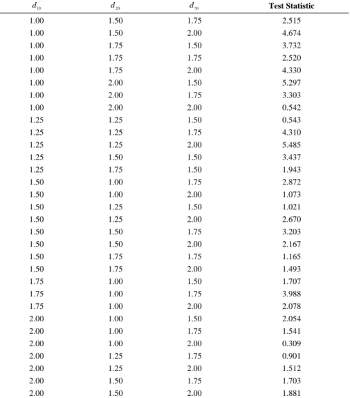
(10) 144. International Journal of Business and Economics. The significance of results in Table 2 might be largely due to failing to account for I (0) autocorrelation in u t . Thus, we fit a VAR(1) structure for the disturbances. The results are displayed in Table 3; they are very similar to those in Table 2 but the proportion of non-rejection values is a higher in Table 3. In fact, the non-rejection values in Table 2 form a proper subset of the non-rejection values in Table 3. They range between 1 and 2 for d10 , between 1.25 and 2 for d 20 , and between 1.50 and 2 for d30 . Thus, using the multivariate tests, we obtain conclusions very similar to those based on univariate test: we observe higher orders of integration for the UK than for the US, and the highest values for Canada, implying a stronger degree of dependence between the observations in Canada with respect to the US or the UK. Table 3. Values of d where H 0 Cannot Be Rejected at the 5% Level: VAR(1) Disturbances. d 10. d 20. d 30. Test Statistic. 1.00. 1.50. 1.75. 2.515. 1.00 1.00. 1.50 1.75. 2.00 1.50. 4.674 3.732. 1.00 1.00 1.00. 1.75 1.75 2.00. 1.75 2.00 1.50. 2.520 4.330 5.297. 1.00 1.00. 2.00 2.00. 1.75 2.00. 3.303 0.542. 1.25 1.25 1.25. 1.25 1.25 1.25. 1.50 1.75 2.00. 0.543 4.310 5.485. 1.25 1.25 1.50 1.50 1.50 1.50 1.50 1.50 1.50 1.50 1.75 1.75 1.75 2.00 2.00 2.00 2.00 2.00 2.00 2.00. 1.50 1.75 1.00 1.00 1.25 1.25 1.50 1.50 1.75 1.75 1.00 1.00 1.00 1.00 1.00 1.00 1.25 1.25 1.50 1.50. 1.50 1.50 1.75 2.00 1.50 2.00 1.75 2.00 1.75 2.00 1.50 1.75 2.00 1.50 1.75 2.00 1.75 2.00 1.75 2.00. 3.437 1.943 2.872 1.073 1.021 2.670 3.203 2.167 1.165 1.493 1.707 3.988 2.078 2.054 1.541 0.309 0.901 1.512 1.703 1.881.

(11) Luis A. Gil-Alana. 145. Finally, it might also be of interest to examine the cross-correlation across countries in those cases where the null hypothesis cannot be rejected. Though the values are not reported, it was observed that the highest values in the variancecovariance matrices were obtained for the cases of the US and Canada and the US and the UK, while the lowest values corresponded to the relationship between the UK and Canada. All this is consistent with the empirical fact observed in the economic activity that the US and Canada and the US and UK are more economically related than Canada and the UK. In any case, the fact that the three orders of integration are higher than 1 suggests that there is no mean reversion in any of the series, with shocks that affect them persisting forever without strong policy action to bring them back to their original levels. 5. Concluding Comments. In this paper we propose a multivariate long memory model and extend the univariate tests of Robinson (1994). We use this method to test the orders of integration of real output in the US, the UK, and Canada in a multivariate system. However, as a preliminary step, we also performed univariate analyses. Using the parametric procedure of Robinson (1994), the results decisively reject the unit root null hypothesis for all series, especially for Canada, in favor of higher orders of integration. Using a univariate semiparametric method (Robinson, 1995), which is robust to the different types of disturbances, the evidence was also strong against the existence of unit roots. Thus, the univariate work emphasizes the non-stationary nature of the series and the lack of mean-reverting behavior. The results based on the multivariate procedure corroborate the univariate results, finding conclusive evidence against mean reversion for the three countries. Moreover, they stress once more the fact that Canada presents higher orders of integration than the other two countries, implying that stronger policy actions must be required in this country to bring output to its original long-term projection. Finally, looking at the covariance matrices of the differenced series, the results show that the US and Canada and the US and UK are more related than Canada and the UK, an observation that should be expected in view of the major economic relationships between these countries. Similar to the univariate tests of Robinson (1994), the multivariate tests presented in this paper also permit us to incorporate deterministic components (e.g., intercepts, linear trends, or seasonal dummies), with no effect on its standard null limit distribution. However, the inclusion of these components did not alter the conclusions presented here; we obtain very similar results in favor of nonstationarity and lack of mean-reverting behavior in the real output of the three countries. Finally, the diagonal matrix appearing in (6) can also be extended to the non-diagonal case, and, though the functional form of the test statistic is much more complicated in this context, it would permit us to study the case of cointegration from a different (fractional) time series perspective. Work in this direction is now in progress..

(12) 146. International Journal of Business and Economics. References. Agiakloglou, C. and P. Newbold, (1994), “Lagrange Multiplier Tests for Fractional Difference,” Journal of Time Series Analysis, 15, 253-262. Bloomfield, P., (1973), “An Exponential Model in the Spectrum of a Scalar Time Series,” Biometrika, 60, 217-226. Dickey, D. A. and W. A. Fuller, (1979), “Distribution of the Estimators for Autoregressive Time Series with a Unit Root,” Journal of the American Statistical Association, 74, 427-431. Gil-Alana, L. A., (2003a), “Multivariate Tests of Nonstationary Hypothesis,” South African Statistical Journal, 37, 1-28. Gil-Alana, L. A., (2003b), “A Fractionally Multivariate Long Memory Model for the US and the Canadian Real Output,” Economics Letters, 81, 355-359. Kwiatkowski, D., P. C. B. Phillips, P. Schmidt, and Y. Shin, (1992), “Testing the Null Hypothesis of Stationarity against the Alternative of a Unit Root,” Journal of Econometrics, 54, 159-178. Phillips, P. C. B. and P. Perron, (1988), “Testing for a Unit Root in a Time Series Regression,” Biometrika, 75, 335-346. Robinson, P. M., (1991), “Testing for Strong Serial Correlation and Dynamic Conditional Heteroskedasticity in Multiple Regression,” Journal of Econometrics, 47, 67-84. Robinson, P. M., (1994), “Efficient Tests of Nonstationary Hypotheses,” Journal of the American Statistical Association, 89, 1420-1437. Robinson, P. M., (1995), “Gaussian Semiparametric Estimation of Long Range Dependence,” Annals of Statistics, 23, 1630-1661. Sowell, F., (1992), “Maximum Likelihood Estimation of Stationary Univariate Fractionally Integrated Time Series Models,” Journal of Econometrics, 53, 165-188. Tanaka, K., (1999), “The Nonstationary Fractional Unit Root,” Econometric Theory, 15, 549-582..

(13)