A Scalable Cluster-based Manycast in Ad Hoc Networks

全文

(1)Int. Computer Symposium, Dec. 15-17, 2004, Taipei, Taiwan.. A Scalable Cluster-based Manycast in Ad Hoc Networks Shiow-Fen Hwang+, Jiang-Jiun Lin*, Kun-Hsien Lu*, and Chyi-Ren Dow+ Department of Information Engineering and Compuetr Science Feng Chia Unverisity, Taichung, Taiwan 407, R.O.C. +Email: {sfhwang, [email protected]} *Email: {m9113224, [email protected]} communication mechanism called manycast and declared that manycast must be implemented in network layer to support the service-oriented group communication. Different to multicast, manycast is a group communication scheme where one client communicates simultaneously with some threshold number k of servers from the m servers of a group. Moreover, manycast provides a simple request/reply communication between a client and servers. The activities of manycast transaction are shown in Fig. 1.. Abstract--Sources and services providing is a topical network application nowadays and in the future. Comparing with traditional wired networks, it is more important and difficult for ad hoc networks to design an applicable communication pattern to provide services. As the appearance of services becomes complex, some traditional group communication mechanisms such as multicast or anycast may not satisfy some kinds of services like NTP (Network Time Protocol). Manycast is a group communication paradigm in which one client communicates simultaneously with k of m equivalent servers in a group. Although some protocols like scoped-flood have been proposed to perform manycast delivery, while they still suffer from the problem of redundant transmission overhead. Hence, we propose a scalable clusterbased manycast to reduce those overhead but still keep a high successful ratio of manycast delivery.. MANET service provider Wireless link. Keywords: Ad Hoc Network, Manycast, Service, Clustering.. MANET device Service request. Service reply. Figure 1. The activity of manycast transaction Although flooding or some on-demand routing protocols in ad hoc networks can be modified to perform manycast delivery mechanisms. However, C. Cater et al. [2] recommended the scoped-flood mechanism because it keeps the merit of flooding which can resist mobility and save a number of retransmission overhead in their simulation environment. But the scoped-flood still suffers from some flaws including the embarrassment of the TTL (timeto-live) setting (scoped area), the server reply implosion, and the scalability problem. The scoped-flood uses flooding to the whole network to perform manycast delivery when a client sends a manycast request at the first time, and then to set TTL value for future usage. However, the flooding may cause the redundant rebroadcasts, contentions, and collisions, which are known as the broadcast storm problem [5] in MANETs. A client may use the TTL value to limit the flood area at the next manycast request. Unfortunately, it may occur that the evaluated TTL value becomes inaccurate due to the mobility of hosts. Second, the reply implosion problem will happen such as the ARP implosion [1] if there are too many servers received a manycast request and reply it. Finally, considering the scalability of network environment, if the network size extends and the number of hosts and. 1. Introduction A mobile ad hoc network (MANET) [9] is a network consisting of a number of wireless mobile hosts which can move around at will. The data transmission can be accomplished via the nearby mobile hosts interchanging messages. The kind of networks is specially important and useful in the regions without base station supporting such as in battlefield or disaster area. Recently, the network environment can offer a large number of services and resources to users such as the multimedia information service, file-sharing service, or print service, etc. Besides, there are many applications which are to find some equivalent servers in the networks, such as the Network Information System (NIS) in UNIX system, Remote Procedure Call (RPC), Network Time Protocol (NTP) [10] which a client needs to discovery three optimal servers to synchronize its clock, the ITTC (Intrusion Tolerance via Threshold Cryptography) project [6] which a client must contact several servers simultaneously to obtain a complete secret key , MOCA (Mobile Certificate Authority) [7], and COCA (Cornell On-line Certificate Authority) [8], etc. Hence, C. Cater et al. [2] proposed a novel group. 833.

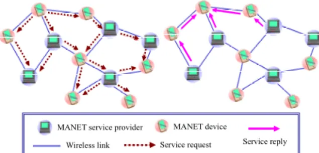
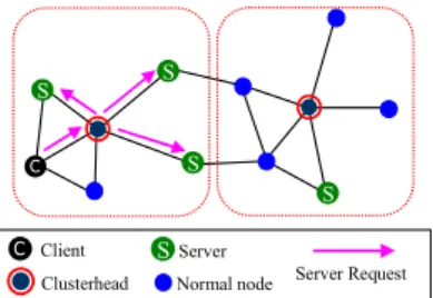
(2) Int. Computer Symposium, Dec. 15-17, 2004, Taipei, Taiwan. kc where c is a constant, 0≦c＜1, to increase the probability of finding at least k servers. The client which wants to perform manycast will send a Server_Request(K) to its clusterhead. After the clusterhead received the Server_Request(K), it will check the number of servers, it dominates, say s. And then, the clusterhead will decide whether transmit it by the following rules. Case 1: s ≧ K The number of requested servers is sufficient in the client’s cluster. The corresponding clusterhead no longer need to transmit the request to other clusters. It only informs all of the servers it dominates to respond a reply to the client. An example which assumed the number of requested servers is two is shown in Fig. 2.. servers increases, the performance of scoped-flood will dramatically drop due to the increase of redundant transmission overhead. In order to improve the defects described above, we use the clustering technique to control the manycast request packets, and therefore propose an efficient manycast scheme in this paper. The rest of the paper is constructed as follows. In section 2, we propose our cluster-based manycast algorithm, including the clustering we adapted and how the manycast works in the cluster. In section 3, we show the simulated results to evaluate the performance of our scheme and compare with scoped-flood [2]. Finally, the conclusions are drawn and some directions for future work are presented in section 4.. 2. A Cluster-based Manycast If a client wants to use scoped-flood to perform manycast to reach the required m servers, there will be a large numbers of overheads because of the redundant transmissions and replies. Therefore, we adopt cluster hosts in the network to efficiently reduce manycast request packets and find the required m servers more accurately by the managemant of clusterheads.. S. S. S. C. S C Client Clusterhead. S. Server Normal node. Server Request. Figure 2. The number of requested servers is enough in the intra cluster.. 2.1 The Clustering Among most clustering algorithms, one of criteria to judge whether the clustering algorithm is good or not is the frequency of cluster changes. If the frequency of cluster changes is less, it means that the cluster structure is more stable. Hence, we adopt the Least Cluster Change Algorithm (LCC) proposed by C.-C. Chiang [3] to construct and maintain the cluster. The advantanges of LCC algorithm is that it improve the problem of the most common clustering algorithms such as Lowest-ID (LID) clustering or Highest-Connectivity (HCC) clustering, in which the numbe of clusterheads will increase as time goes by. Hence, the LCC algorithm not only has the merit of simpilicity and quick construction in LID or HCC clustering, but also decreases the variant frequences of these two algorithms.. 2.2 Our Manycast Scheme In the section, we introduce our cluster-based manycast in two phases. In the server request phase, we describe how to control server request packet propagations, and how to find at least k servers. In the server reply phase, we describe how the servers reply to the client when receiving the request packets. 2.2.1 Server Request Assume that a certain client in the network requests k servers from m servers (k≦m) for service, and these servers who received the request must respond a reply back to the client. First, we set K = k +. Case 2：s ＜ K The situation means that there are not enough servers in the client’s cluster. Hence, the clusterhead will inform the servers in its cluster to reply to the client and also exchange the information by gateways to obtain the number of servers in its neighbor clusters. Assume that the total number of servers in the neighbor clusters is g. (i) s + g ≧ K The required number of servers is sufficient among the client’s cluster and neighbor clusters. At this time, the clusterhead informs all its neighbor clusterheads, and then they will inform all the servers in their clusters to reply to the client as soon as possible. For example, in the Fig. 3, we assume the number of requested servers is 6. After examining the number of servers, among its cluster and neighbor clusters, which is 9, the client’s clusterhead will inform the servers within it and transmit the request with T = 0 to its neighbor clusterheads. (ii) s + g ＜ K The required number of servers is not satisfied both in the client’s cluster and the neighbor clusters. The responsibility for searching the remainder insufficient servers will be took by the neighbor clusters. Let T = ⎡⎢( K − s − g ) p ⎤⎥ , where p is the number of neighbor clusters of the client’s cluster. The clusterhead of the client will inform its neighbor clusterheads with piggybacked T. As receiving the request, the clusterheads will firstly inform the servers in their clusters to reply to the client. And then they exchange. 834.

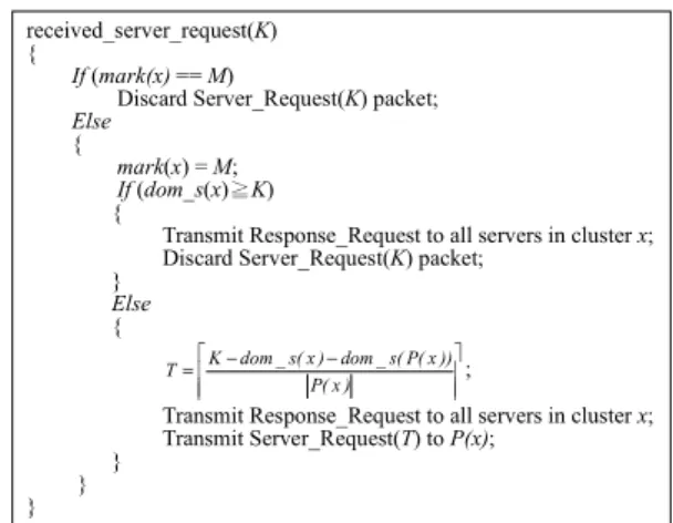
(3) Int. Computer Symposium, Dec. 15-17, 2004, Taipei, Taiwan. the information with gateways to decide whether the transmission is necessary and avoid the replicated assignment to the same neighbors if the transmission is necessary. Finally, neighbor clusters will recompute the T based on their unmarked neighbor clusters to distribute the responsibility to these clusters to find the T servers. If an unmarked neighbor clusterheads receive the request, it will repeat the steps described above. In the example of Fig. 4, because the number of requested servers is equal to 14 which is larger than total servers in the client’s cluster and its neighbor clusters. The cluster, then, will transmit the request with T=2 to its neighbor clusters. After cluster 1, 2, and 3 received the request, they then investigate the number of its unmarked neighbor clusters and transmit the request packet to them with the recomputed T. Consequently, these clusters will decide what to do depending on the cases described above. S. S. z z z z. While the clusterhead x receives the Server_Request(K) from a client, it will perform the algorithm I described in Fig. 5.. S. received_server_request(K) { If (mark(x) == M) Discard Server_Request(K) packet; Else { mark(x) = M; If (dom_s(x)≧K) { Transmit Response_Request to all servers in cluster x; Discard Server_Request(K) packet; } Else {. S. S. C. S. z. S S. S. ⎡ K − dom _ s( x ) − dom _ s( P( x )) ⎤ T =⎢ ⎥; P( x ) ⎢ ⎥. S Server. C Client Clusterhead. Server Request. Normal node. Figure 3. The number of requested servers is enough in the intra cluster and neighbor ones.. }. T=2 T=2. S. T=2. S. S. S S. T=2. S. 3 T=1. C Client Clusterhead. received_server_request(T) { If (mark(x) == M) Discard Server_Request(T) packet; Else { mark(x) = M; If (T == 0) { Transmit Response_Request to all servers in cluster x; Discard Server_Request(T) packet; } Else {. S. 1. C. }. While the clusterhead x receives the Server_ Request(T) from its neighbor clusters, it will perform the algorithm II described in Fig. 6.. S. 2. }. Transmit Response_Request to all servers in cluster x; Transmit Server_Request(T) to P(x);. Figure 5. Algorithm I of manycast for server request phase.. T=2 S. S. k servers adding to a parameter (kc) to increase the likelihood of reliable manycast delivery. Response_Request ： when a clusterhead x receive the Server_Request(K), the clusterhead use the packet to inform the servers it dominates and the gateways to exchange informations. dom_s(x)：the number of servers a clusterhead x dominates. P(x)：for a clusterhead x, the set of its neighbor clusters which have not been marked. dom_s(P(x))：the summation of the number of servers which are dominated by the nodes of P(x). mark(x)：it record the state of the clusterhead x whether has been assigned to search servers. The state is marked as M if the assignment is true. Otherwise, it is marked as U.. S. ⎡ T ⎤ T =⎢ ⎥; ⎢ P( x ) ⎥. S Server Normal node. Server Request. Figure 4. The number of requested servers is not enough in the inter cluster and neighbor ones.. }. }. }. Transmit Response_Request to all servers in cluster x; Transmit Server_Request(T) to P(x);. Figure 6. Algorithm II of manycast for server request phase.. The detailed algorithm about our scalable clusterbased manycast as explained in the following paragraph. We first define some terms that will be used in the algorithms. z Server_Request(K)：a request which is initialized by a client. The K value means the requested. 2.2.2 Server Reply As receiving the Response_Request packet, a server must reply a packet back to the client. In our. 835.

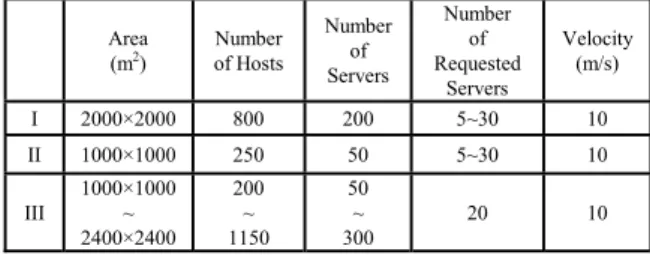
(4) Int. Computer Symposium, Dec. 15-17, 2004, Taipei, Taiwan. work, we assume that the data communication between the client and servers is reactive and brief. If the communication is constant, it is worth to find an efficient path between them, but it is not our issue. We just use a simple method like DSR [4] unicast routing to implement the server reply phase. Whenever a host (a clusterhead or a gateway) transmits the server request to it neighbor clusters, its ID will piggyback in the packet header. After a server received this packet, the reply can traverse the reverse path recorded in the header back to the client. However, because in our scheme, the traversing path is only along in the cluster structure, the path must be a form of cluster to gateway and gateway to cluster. Hence the reply path will be longer as well as response time. For this reason, the path shorten is applied in our scheme. As receiving a reply, the host will check its neighbor and the packet header to see if there is a neighbor which is closer to the next hop recorded in the header. If it is true, the path can be shorten. For example, in Fig. 7, client C initializes a manycast request. After the request traverses along the path and reach a certain server, the server replies the request by the reverse path which is recorded in the header of request packet. In the example, the reverse path is S-4-3-2-1-C. However, it is clear that host S can directly communicate with host 3 without the relay by node 4, and so does host 2.. 2. According to the parameters set above, we experiment several different scenarios as shown in Table 1. Table 1. Simulation parameters in three scenarios.. Clusterhead. S Server Normal node. 4. Server Request. 800. 200. 1000×1000. 250. 50. 5~30. 10. III. 1000×1000 ~ 2400×2400. 200 ~ 1150. 50 ~ 300. 20. 10. Number of Servers. Velocity (m/s) 10. Server Reply. 3.2 Scenario II. Figure 7. Shorten the reply path.. In this section, we simulate in a smaller environment to examine whether our SCM is scalable or not. The experimental results are presented in Fig. 12 ~ Fig. 15. For successful ratio, the performance is similar to the large size of network environment However, in smaller network areas; the cluster brings fewer advantages into the manycast because the constructed cluster numbers are fewer. The savings of manycast overhead does not outperform well in the area compared to the larger network size.. 3. Simulation Results In this section, we compare our scalable clusterbased manycast(SCM) with scoped-flood by the following metrics:(1)Successful Ratio-the percentage of total successful replies over the total manycast requests issued. (2)Manycast Overhead-the average numbers of transmissions per manycast request. (3)Average Servers Replied-the average number of total replies from servers per manycast request. (4)Average Hop Count-the average number of total hop counts in the first k shortest replying paths per manycast request. The simulation environment is as follows: z z z z z z z. 2000×2000. II. Number of Hosts. As shown in Fig. 8, because scoped-flood sets the TTL relying on a beforehand flooding, the inaccurate TTL caused by host mobility will make the successful ratio drop. Besides, Fig. 9 shows that, depending on the clustering, our SCM has better improvement on manycast overhead. On the contrary, scoped-flood needs beforehand flooding and has no management of clusterheads to limit the disseminations of request packets. The manycast overhead is greatly higher than our SCM. In addition, more request packets propagation to servers also incurs many servers reply, which causes the manycast overhead increase. This phenomenon is presented in Fig. 10. However, the scoped-flood performs better in the average hop count metric because shortest paths are traversed, but the difference is not too much, as shown in Fig. 11.. C. C Client. I. Number of Requested Servers 5~30. Area (m2). 3.1 Scenario I. S. 3. 1. z Mobility Model: Random waypoint with pause time 10s. z K: k+1(in scoped-flood). z Percentage of c: (1) fixed 0%. (2) fixed 10%. (3) initially, c＝0 % for all host. Once a request fails, it adjusts to 10% for the next time.. 3.3 Scenario III In Fig. 16, the simulation result indicates that the successful ratio is not affected by the network scale in SCM. In Fig. 17, because the scoped-flood algorithm need all of the nodes within the TTL range to transmit or relay manycast packets, the manycast overhead metric become greater with the growth of network size and server density. Besides, the numbers of replied servers also substantially increase since the usage of flooding to calculate the TTL value in Fig. 18.. Simulation area: 1000m×1000m~2400m×2400m. Number of mobile hosts: 200~1150. Transmission range: 250m. Number of requested servers: 5~30. Number of manycast request issued: 400~2300. Simulation time: 200s~1150s. Mobility speed: 0~20 m/s.. 836.

(5) Int. Computer Symposium, Dec. 15-17, 2004, Taipei, Taiwan. tion authority,” in Proc. of ACM Transactions on Computer Systems, Vol. 20, No. 4, pp.329368, Nov. 2002. [9] Mobile Ad-hoc Networks (manet) working group of IETF, http://www.ietf.org/html.chart ers/manet-charter .html. [10] Network Time Protocol (NTP) Version 4, http://www.ntp.org.. However, in our SCM, manycast packets are only transmitted or relayed by servers, clusterheads, and gateways. The manycast overhead only has a little increase when network size becomes larger, and so as the average replied servers. The average hop count metric of SCM just has a little larger than scopedflood as shown in Fig. 19.. 4. Conclusions and Future Work. 2000×2000, 800 Nodes, 200 Servers, Request 1000 times. We propose a scalable cluster-based manycast to perform manycast delivery. First, based on the structure of cluster, our scheme saves a large number of extra overheads in comparison with scoped-flood without losing the reachability of servers reply. The simulation results show that our SCM scheme performs well when the network environment is dense (higher node/server density). In the future, we will investigate the server reply phase of manycast when the communication between the client and servers is constant. Under these considerations, stable paths should be established rather than using the reverse path that the server request packet traverses.. 1.00 0.99. Succesful Ratio. 0.98 0.97 0.96 0.95 0.94 0.93 0.92 0.91. SCM SCM 0 to 10%. Scoped-Flood SCM 10%. 0.90 5. 10. 15. 20. 25. 30. Requested Servers. Figure 8. Successful ratio vs. requested servers in scenario I. 2000×2000, 800 Nodes, 200 Servers, Request 1000 times. 837. SCM SCM 0 to 10%. 5. 10. 15. 20. Scoped-Flood SCM 10%. 25. 30. Requested Servers. Figure 9. Manycast overhead vs. requested servers in scenario. 2000×2000, 800 Nodes, 200 Servers, Request 1000 times. 120. Average Servers Replied. 100 80 60 40 20. SCM SCM 0 to 10%. Scoped-Flood SCM 10%. 0 5. 10. 15. 20. 25. 30. Requested Servers. Figure 10. Average servers replied vs. requested servers in scenario I. 2000×2000, 800 Nodes, 200 Servers, Request 1000 times. 2.5 2.0 Average Hop Count. [1] C. Carter, S. Yi, and R. Kravets, “ARP considered harmful: manycast transactions in ad hoc networks,” in Proc. of the IEEE wireless Communications and Networking Conference, Vol. 3, pp. 1801-1806, 2003. [2] C. Carter, S. Yi, and R. Kravets, “Manycast: exploring the space between anycast and multicast in ad hoc networks,” in Proc. of the 9th annual international conference on Mobile computing and networking, pp. 273-285, 2003. [3] C.-C. Chiang, H.-K. Wu, W. Liu and M. Gerla, Routing in clustered multihop, mobile wireless networks with fading channel, in Proc. of IEEE Singapore Int. Conf. on Networks, pp. 197-211. [4] D. B. Johnson, D. A. Maltz, and Y.-C. Hu, “The Dynamic Source Routing Protocol for Mobile Ad Hoc Networks (DSR)” Mobile Ad-hoc Networks (manet) working group of IETF, http://www.ietf.org/internet-drafts/draft-ietf-ma net-dsr- 09.txt, April 2003. [5] S.-Y. Ni, Y.-C. Tseng, Y.-S. Chen, and J.-P. Sheu, “The broadcast storm problem in a mobile ad hoc network,” Wireless Networks, Vol. 8, No. 2, pp. 153-167, March 2002. [6] T. Wu, M. Malkin, and D. Boneh, “Building intrusion tolerant applications,” in Proc. of the 8th USENIX Security Symposium, pp. 79-91, 1999. [7] S. Yi and R. Kravets, “MOCA: Mobile certificate authority for wireless ad hoc networks,” in Proc. of the 2nd Annual PKI Research Workshop, April 2003. [8] L. Zhou, F. B. Schneider, and R. van Renesse, “COCA: A secure distributed on-line certifica-. Manycast Overhead. References. 1100 1000 900 800 700 600 500 400 300 200 100 0. 1.5 1.0 0.5. SCM SCM 0 to 10%. Scoped-Flood SCM 10%. 0.0 5. 10. 15. 20. 25. 30. Requested Servers. Figure 11. Average hop count vs. requested servers in scenario I..

(6) Int. Computer Symposium, Dec. 15-17, 2004, Taipei, Taiwan.. 1.00. 1.00 0.99 0.98 0.97 0.96 0.95 0.94 0.93 0.92 0.91 0.90 0.89 0.88. 0.99 0.98 0.97. Succesful Ratio. Succesful Ratio. 1000×1000, 250 Nodes, 50 Servers, Request 500 times. 0.96 0.95 0.94 0.93 0.92. SCM SCM 0 to 10%. 5. 10. Scoped-Flood SCM 10%. 15. 0.91. 20. 25. SCM. Scoped-Flood. SCM 0 to 10%. SCM 10%. 0.90 1000×1000 1200×1200 1400×1400 1600×1600 1800×1800 2000×2000 2200×2200 2400×2400. 30. Network Size(m2). Requested Servers. Figure 16. Successful ratio vs. square network size in scenario III.. Figure 12. Successful ratio vs. requested servers in scenario II.. 1200 1100. 350. 1000. 300. 900. SCM. Scoped-Flood. SCM 0 to 10%. SCM 10%. 800. 250. Manycast Overhead. Manycast Overhead. 1000×1000, 250 Nodes, 50 Servers, Request 500 times. 200 150 100 50. SCM SCM 0 to 10%. 10. 15. 20. 25. 600 500 400 300 200. Scoped-Flood SCM 10%. 100. 0 5. 700. 0 1000×1000 1200×1200 1400×1400 1600×1600 1800×1800 2000×2000 2200×2200 2400×2400. 30. Requested Servers. 2. Network Size(m ). Figure 13. Manycast overhead vs. requested servers in scenario II.. Figure17. Manycast overhead vs. square network size in scenario III. 130 120. 45. 110. 40. 100. 35. 90. Average Servers Replied. Average Servers Replied. 1000×1000, 250 Nodes, 50 Servers, Request 500 times. 30 25 20 15 10 SCM SCM 0 to 10%. 5. Scoped-Flood SCM 10%. 80 70 60 50 40 30 20 10. 0 5. 10. 15. 20. Requested Servers. 25. SCM. Scoped-Flood. SCM 0 to 10%. SCM 10%. 0 1000×1000 1200×1200 1400×1400 1600×1600 1800×1800 2000×2000 2200×2200 2400×2400. 30. Network Size(m2). Figure 18. Average servers replied vs. square network size in scenario III.. Figure 14.Average servers replied vs. requested servers in scenario II.. 2.00. 1000×1000, 250 Nodes, 50 Servers, Request 500 times. 1.80. 2.5. 1.60 1.40. Average Hop Count. Average Hop Count. 2.0 1.5 1.0 0.5. SCM SCM 0 to 10%. Scoped-Flood SCM 10%. 1.20 1.00 0.80 0.60 0.40 0.20. 0.0 5. 10. 15. 20. 25. SCM. Scoped-Flood. SCM 0 to 10%. SCM 10%. 0.00 1000×1000 1200×1200 1400×1400 1600×1600 1800×1800 2000×2000 2200×2200 2400×2400. 30. Requested Servers. Network Size(m 2). Figure 15. Average hop count vs. requested servers in scenario II.. Figure 19. Average hop count vs. square network size in scenario III.. 838.

(7)