A 2-approximation algorithm for the SROCT problem
∗Bang Ye Wu Kun–Mao Chao
Problem: Optimal Sum-Requirement Communication Spanning Trees (SROCT) Instance: A G = (V, E, w) with vertex weight r : V → Z0+.
Goal: Find a spanning tree T of minimum s.r.c. cost.
Recall that the s.r.c. routing cost of a tree T is defined by Cs(T ) = P
u,v(r(u) + r(v))dT(u, v). Similar to the PROCT problem, the SROCT problem includes the MRCT problem as a special case and is therefore NP-hard. The s.r.c. cost of a tree can also be computed by summing the routing costs of edges. The only difference is the definition of routing load.
Definition 1: Let T be any spanning tree of a graph G, and r a vertex weight function. For any edge e = (u, v) ∈ E(T ), we define the s.r.c. routing load on the edge e to be ls(T, r, e) = 2(r(Tu)|Tv| + r(Tv)|Tu|), where Tu and Tv are the two subgraphs obtained by removing e from T . The s.r.c. routing cost on the edge e is defined to be ls(T, r, e)w(e).
Lemma 1: Let T be any spanning tree of a graph G = (V, E, w) and r be a vertex weight function. Cs(T ) =Pe∈E(T )ls(T, r, e)w(e).
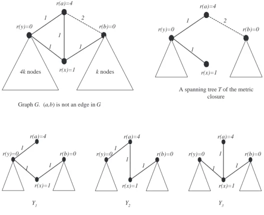
In this section, we focus on the approximation algorithm for an SROCT. For the PROCT problem, it has been shown that an optimal solution for a graph has the same value as the one for its metric closure. In other words, using bad edges cannot lead to a better solution. However, the SROCT problem has no such a property. For example, consider the graph G in Figure 1. The edge (a, b) is not in E(G), and T is a spanning tree of the metric closure of G. All three possible spanning trees of G are Y1, Y2 and Y3. It will be shown that the s.r.c cost of T is less than that of Yi for i = 1, 2, 3.
To compare the s.r.c costs, we can only focus on the coefficient of k in the cost. Note that only vertices a and x have nonzero weights. By Lemma 1, the s.r.c. cost of T can be computed as follows:
Cs(T )
= ls(T, r, (a, b))w(a, b) + ls(T, r, (a, y))w(a, y) + ls(T, r, (y, x))w(x, y) = 2(k(4 + 1) + 0(4k))2 + 2(k × 1 + 4 × 4k)(1) + 2(5k × 1 + 4 × 1)(1) = 64k + . . .
Similarly we have Cs(Y1) = 66k, Cs(Y2) = 66k, and Cs(Y3) = 90k. The example illustrates that it is impossible to transform any spanning tree of ¯G to a spanning tree of G without increasing the s.r.c cost for some graph G, where ¯G is the metric closure of G. But it should be noted that the
∗An excerpt from the book “Spanning Trees and Optimization Problems,” by Bang Ye Wu and Kun-Mao Chao
(2004), Chapman & Hall/CRC Press, USA.
4k nodes r(y)=0 r(x)=1 r(a)=4 r(b)=0 1 1 1 1 2 k nodes r(y)=0 r(x)=1 r(a)=4 r(b)=0 1 1 2 r(y)=0 r(x)=1 r(a)=4 r(b)=0 1 1 1
Graph G. (a,b) is not an edge in G
A spanning tree T of the metric closure r(y)=0 r(x)=1 r(a)=4 r(b)=0 1 1 1 r(y)=0 r(x)=1 r(a)=4 r(b)=0 1 1 1 Y1 Y2 Y3
Figure 1: A tree with bad edges may have less s.r.c. cost. The triangles represent nodes of zero weight and connected by zero-length edges.
example does not disprove the possibility of reducing the SROCT problem on general graphs to its metric version.
We shall present a 2-approximation algorithm for the SROCT problem on general graphs. For each vertex v of the input graph, the algorithm finds the shortest-paths tree rooted at v. Then it outputs the shortest-paths tree with minimum s.r.c. cost. We shall show that there always exists a vertex x such that any shortest-paths tree rooted at x is a 2-approximation solution.
In the following, graph G = (V, E, w) and vertex weight r is the input of the SROCT problem. We assume that |V | = n, |E| = m and r(V ) = R.
Lemma 2: Let T be a spanning tree of G. For any vertex x ∈ V , Cs(T ) ≤ 2 X v∈V (nr(v) + R) dT(v, x). Proof: Cs(T ) = X u,v∈V (r(u) + r(v)) dT(u, v) ≤ X u,v∈V (r(u) + r(v)) (dT(u, x) + dT(x, v)) = 2 X u,v∈V (r(u) + r(v)) dT(u, x) ≤ 2X v∈V (nr(v) + R) dT(v, x). 2
In the following, we use T to denote an optimal spanning tree of the SROCT problem, and use x1 and x2 to denote a centroid and an r-centroid of T respectively. Let P = SPT(x1, x2) be the path between the two vertices on the tree. If x1 and x2 are the same vertex, P contains only one vertex.
Lemma 3: For any edge e ∈ E(P ), the s.r.c load ls(T, r, e) ≥ nR.
Proof: Let T1and T2be the two subtrees resulting by deleting e from T . Assume that x1 ∈ V (T1) and x2 ∈ V (T2). By the definitions of centroid and r-centroid, |V (T1)| ≥ n/2 and r(T2) ≥ R/2. Then,
ls(T, r, e)/2 = |V (T1)|r(T2) + |V (T2)|r(T1)
= |V (T1)|r(T2) + (n − |V (T1)|) (R − r(T2))
= 2 (|V (T1)| − n/2) (r(T2) − R/2) + nR/2 ≥ nR/2.
The next lemma establishes a lower bound of the minimum s.r.c. cost. Remember that dT(v, P ) denotes the shortest path length from vertex v to path P .
Lemma 4: Cs(T ) ≥Pv∈V (nr(v) + R) dT(v, P ) + nRw(P ).
Proof: For any vertex u, we define SB(u) to be the set of vertices in the same branch of u. Note that |SB(u)| ≤ n/2 and r(SB(u)) ≤ R/2 for any vertex u by the definitions of centroid and r-centroid. Cs(T ) = X u,v∈V (r(u) + r(v)) dT(u, v) = 2 X u,v∈V r(u)dT(u, v) ≥ 2X u∈V X v /∈SB(u) r(u) (dT(u, P ) + dT(v, P )) +2 X u,v∈V r(u)w(SPT(u, v) ∩ P ). (1)
For the first term in (1),
2X u∈V X v /∈SB(u) r(u) (dT(u, P ) + dT(v, P )) = 2X u∈V X v /∈SB(u) r(u)dT(u, P ) + 2 X u∈V X v /∈SB(u) r(u)dT(v, P ) ≥ X u∈V nr(u)dT(u, P ) + 2X v∈V X u /∈SB(v) r(u)dT(v, P ) ≥ X u∈V nr(u)dT(u, P ) + X v∈V RdT(v, P ) = X v∈V (nr(v) + R) dT(v, P ). (2) 3
For the second term in (1), 2 X u,v∈V r(u)w(SPT(u, v) ∩ P ) = 2 X u,v∈V r(u) X e∈SPT(u,v)∩P w(e) = X e∈E(P ) Ã 2X v
r ({u|e ∈ E(SPT(u, v))}) ! w(e) = X e∈E(P ) ls(T, r, e)w(e) ≥ nRw(P ). (by Lemma 3) (3)
The result follows (1), (2), and (3).
The main result of this section is stated in the next theorem.
Theorem 5: There exists a 2-approximation algorithm with time complexity O(n2log n + mn) for the SROCT problem.
Proof: Let Y∗ and Y∗∗ be the shortest-path trees rooted at x
1 and x2 respectively. Also, for any v ∈ V , let h1(v) = w(SPT(v, x1) ∩ P ) and h2(v) = w(SPT(v, x2) ∩ P ). By Lemma 2,
Cs(Y∗)/2 ≤ X v∈V (nr(v) + R) dY∗(v, x1) ≤ X v∈V (nr(v) + R) (dT(v, P ) + h1(v)). (4) Similarly Cs(Y∗∗)/2 ≤X v∈V (nr(v) + R) (dT(v, P ) + h2(v)). (5)
Since h1(v) + h2(v) = w(P ) for any vertex v, by (4) and (5), we have min{Cs(Y∗), Cs(Y∗∗)} ≤ (Cs(Y∗) + Cs(Y∗∗)) /2 ≤ X v∈V (nr(v) + R) (2dT(v, P ) + h1(v) + h2(v)) = X v∈V (nr(v) + R) (2dT(v, P ) + w(P )) = 2X v∈V (nr(v) + R) dT(v, P ) + 2nRw(P ) ≤ 2Cs(T ). (by Lemma 4)
We have proved that there exists a vertex x such that any shortest-paths tree rooted at x is a 2-approximation solution. Since it takes O(n log n+m) time to construct a shortest-paths tree rooted at a given vertex and the s.r.c cost of a tree can be computed in O(n) time, a 2-approximation solution of the SROCT problem can be found in O(n2log n + mn) time by constructing a shortest-paths tree rooted at each vertex and choosing the one with minimum s.r.c cost.