Short Paper
__________________________________________________
A Robust and Accurate Calibration Method by Computer
Vision Techniques for Coordinate Transformation between
Display Screens and Their Images
*SHENG-WEN JENG+AND WEN-HSIANG TSAI+,#
+
Department of Computer Science National Chiao Tung University
Hsinchu, 300 Taiwan
#Department of Computer Science and Information Engineering
Asia University Taichung, 413 Taiwan
A robust and accurate calibration method for coordinate transformation between display screens and their images is proposed. The images of three specially designed calibration patterns, which are a white rectangle, a black rectangle, and a dot matrix, are captured and processed sequentially to assist achieving robust extraction of relevant fea-tures from the calibration pattern images, especially the border feafea-tures in the image of the display screen. Image analysis techniques of deformable template matching, local thresholding, and inverse distance-weighted interpolation are integrated to perform fea-ture extraction and coordinate transformation to complete the calibration work. Good performance of the proposed method is demonstrated by comparing the experimental results of the method with those of a well-known calibration method.
Keywords: calibration, coordinate transformation, dot-matrix pattern, landmark, de-formable template matching, inverse distance-weighted interpolation
1. INTRODUCTION
Projection screens are used commonly in presentations nowadays [1-5]. The pro-jected image on the screen includes many types of contents. Usually, we use a laser pointer to point out mentioned targets in the image. It is advantageous to design an intel-ligent technique to locate the laser spot on the screen automatically by a computer. Pos-sible applications of this technique include game interfacing, computer screen control, presentation paging control, simulation of clicking by a laser pointer, etc. In this study, we want to use the computer vision technique to solve this problem.
More specifically, after using a visual camera to take an image of a screen on which a laser spot appears, it is desired to design a robust and accurate method by computer vision techniques to measure the position of the laser spot, no matter where the spot ap-Received November 15, 2006; revised March 14, 2007; accepted April 23, 2007.
Communicated by Pau-Choo Chung.
pears and no matter what type of camera is used. To solve this problem, a calibration procedure is needed to build a position relationship between the projection screen and the taken image, followed by a transformation process from the image coordinates to the screen coordinates.
When the display screen is planar, intuitively the resulting issue is a traditional cam-era calibration problem between two planar planes [6]. When applying a traditional cali-bration method, we must know some camera parameters like the focal length of the cam-era, the dimension of the CCD sensor in the camcam-era, and so on. We also have to build a lens distortion model before doing the calibration work [6, 7]. Finally, we have to solve some nonlinear equations to compute the solution for coordinate transformation parame-ters. If there are errors in the computed parameters, such traditional methods will reduce the final coordinate transformation precision. Especially, in the issue of simplifying the calibration computation process, it is usual to use a camera lens distortion model of low-order fitting functions in the radial direction of the lens. The results of the coordinate transformation will usually include unacceptable shift errors near the border of the image. Another kind of traditional method is homographic projection [10], by which the projec-tor may be allowed to be at any pose with respect to the screen plane. However, camera and projector optics are modeled by perspective transformations, and the nonlinear dis-tortion property of the optical lens is not considered.
In this study, we try to remove the above-mentioned drawbacks of traditional cali-bration methods. In particular, we focus on improving the accuracy of the coordinate transformation to eliminate the shift errors near the image border. Also, we simplify the algorithms to avoid complicated calculations in the calibration and coordinate transfor-mation processes. We design three calibration patterns and an algorithm for robust ex-traction of geometric feature points from the calibration pattern images. Using the tech-niques of deformable template matching, local thresholding, and inverse distance- weighted interpolation, we achieve robust feature extraction and accurate coordinate transformations. Good experimental results were obtained, which show the feasibility of the proposed method. The experimental results were also compared with those of a well- known calibration method to show the superiority of the proposed method.
In the remainder of this paper, we describe the proposed method in section 2, show some experimental results in section 3, and make conclusions finally in section 4.
2. PROPOSED METHOD
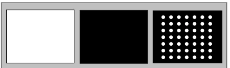
The proposed method includes three stages: (1) taking pictures of calibration pat-terns designed in this study; (2) extracting feature points from the pattern images; and (3) conducting coordinate transformations to accomplish the calibration work. The key idea, which is different from those of traditional calibration methods, is to use sequentially three calibration patterns instead of the conventional way of using only one. The three sequential calibration patterns designed for use in this study are shown in Fig. 1, includ-ing a white rectangular shape, a black rectangular shape, and a matrix of white dots on a black rectangular shape, which are called respectively the white-rectangle pattern, the black-rectangle pattern, and the dot-matrix pattern in the sequel. We capture the images of them, when they are projected on a display screen, with a CCD camera equipped at a
Fig. 1. Calibration patterns − white-rectangle, black-rectangle, and dot-matrix patterns. proper location in the environment, and apply image analysis techniques to extract rele-vant image features for later processing. The images of the white-rectangle pattern and the black-rectangle one are used to extract the border information of the display screen effectively and to create a threshold distribution map (TDM). The border information and the TDM are then used further to assist the extraction of meaningful feature points, called landmark points hereafter, by local thresholding and deformable template match-ing techniques from the dot-matrix pattern image. The landmark points are then used for coordinate transformations by a technique of inverse distance-weighted interpolation. We describe the details in the following sections.
2.1 Use of Calibration Patterns
Fig. 2 shows the captured images of the three calibration patterns displayed on a projection screen. We can see the grayscale value variations in the images caused by un-even environmental lighting. This problem might cause erroneous feature extraction re-sults and so make the calibration work fail. It is solved in this study by a technique of sequential analysis of three calibration pattern images. The advantages of using the white- rectangle pattern and the black-rectangle one in the calibration process include: (1) mak-ing easy and accurate extraction of the border of the display screen from the acquired image; and (2) creating a TDM from these two images for the later effective work of thresholding locally the dot-matrix pattern image into a binary one. The advantages of using the dot-matrix pattern in the calibration process include: (1) providing landmark points in the proposed calibration algorithm; and (2) dividing the display screen images into many small regions for use in the interpolation process which reduces geometric distortions caused by imperfect camera lens optics. If there are N × N dots in the matrix, then we divide the display screen into (N + 2) × (N + 2) small regions, in each of which a coordinate transformation is conducted locally.
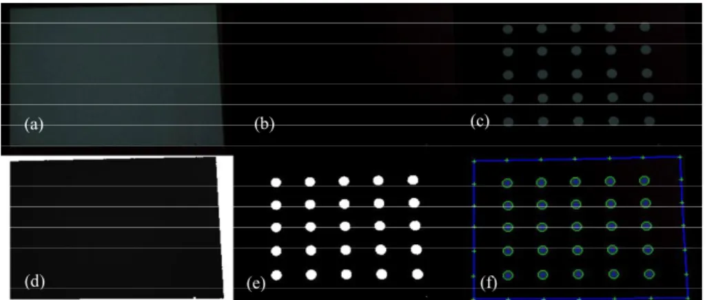
(a) (b) (c) Fig. 2. Examples of captured images of Fig. 1.
The TDM is a grayscale image, each of whose pixels has a threshold value for bi-narizing the pixel value of the dot-matrix pattern image at the corresponding pixel loca-tion. The threshold value at pixel location (i, j) in the TDM can be calculated, according to the concept of local thresholding, from the corresponding pixel locations (i, j) in the white-rectangle and in the black-rectangle pattern images in a way described as follows.
Let the grayscale values at pixel location (i, j) in the white-rectangle and in the black-rectangle pattern images be denoted by w(i, j) and b(i, j), respectively. From the two pattern images as shown in Figs. 2 (a) and (b), we see that the outer parts of the dis-play screen are imaged to be of approximately the same grayscale values, while the white and the black rectangles inside the display screens are imaged to be of great difference in their grayscale values. We define the pixel value t(i, j) of the TDM t at pixel location (i, j) in the following way:
if w(i, j) − b(i, j) > 20, then set t(i, j) = b(i, j) + [w(i, j) − b(i, j)]/2;
else set t(i, j) = 255. (1)
Basically, the above rule defines a threshold value at the middle of the black and the white pixel values in the two patterns, respectively, when there exists an “effective” pixel whose grayscale difference in the two images is large enough (> 20). Otherwise, we set the threshold value to be 255. Fig. 3 shows a TDM created by the images of Figs. 2 (a) and (b).
Fig. 3. A TDM image created by images in Figs. 2 (a) and (b).
The TDM is then used in a process of analyzing a dot-matrix pattern image d by lo-cal thresholding. The aim is to obtain the white dots effectively. The result is a binary dot-matrix pattern image d′ defined by:
if d(i, j) > t(i, j), then set d′(i, j) = 255; else, 0. (2) An example of using the TDM for extracting the dots from the dot-matrix pattern image is shown in Fig. 4 (e). We see in the above process that the use of the white-rec- tangle and the black-rectangle pattern images provides the advantages of removing the outer parts of the display screen and providing local threshold values for binarizing pre-cisely the image of the third calibration pattern, the dot-matrix pattern, into white dots for later processing.
(a) (b) (c)
(d) (e) (f)
Fig. 4. An example of image analysis of dot-matrix pattern image. (a) White-rectangle pattern im-age; (b) Black-rectangle pattern imim-age; (c) Dot-matrix pattern imim-age; (d) TDM; (e) Binary image of (c); (f) Extracted feature points (with marks “+”).
2.2 Feature Extraction
Two kinds of landmark points are then extracted subsequently from the binary dot-matrix pattern image with aids from the original pattern images. The first is the cen-ter of each white dot in the image, which we mention as a dot cencen-terfor simplicity in the sequel. The second kind of extracted landmark point is the intersection point of a screen border line with the line formed by a row or a column of the dot centers in the binary dot- matrix pattern image, which we call an extended dot center in the sequel. For contrast, the first kind of dot center within the dot-matrix pattern image is mentioned as the origi-nal dot center. That is, we now have two types of landmark points now, origiorigi-nal dot center and extended one. These extracted landmark points can be used as anchor points for calibration. They are marked by crosses “+” in Fig. 4 (f). We also see from the results shown in Fig. 4 that the proposed method is quite effective in dealing with non-uniform lighting appearing in the acquired images.
We now describe how we extract these two types of landmark points in more detail. There are three major steps in the extraction process: (a) extraction of the screen border; (b) extraction of the original dot centers; and (c) extraction of the extended dot centers. (a) Extraction of screen border
In order to extract the screen border, we establish a geometric model for the border shape and use an edge matching technique to fit the model, thus obtaining a polygon for use as the shape of the screen border. The main purpose is to have a more precise extrac-tion result of the screen border shape by which the subsequent calibraextrac-tion work can be performed more accurately. More specifically, considering the shape distortion of the rectangular screen in an acquired image caused by imperfect optical geometry of the camera lens, which is mostly barrel or pincushion distortion, we model the screen region in the image as an eight-sided polygon with eight vertexes and eight line segments, de-noted by Pi and Li, respectively, where i = 0, 1, …, 7, as shown in Fig. 5.
F
First, two mutually-perpendicular lines are set at the center of the TDM image, as shown in Fig. 6. A 2 × 6 scan window as shown in Fig. 6 (b) is moved from the TDM image center along the vertical line to its two ends to extract the vertexes P1 and P5 on the upper
and lower border lines, respectively. P3 and P7 on the right and left border lines,
respec-tively, are extracted similarly. Extraction of the vertexes is based on the concept of edge detection using the values of the 12 pixels in each scan window.
Specifically, referring to Fig. 6 (b), let the average grayscale value of the group of the upper six pixels in the window be denoted as G1, and let that of the lower six pixels
as G2. Then, either of the vertexes of P1 and P5 is detected by searching the maximum of
the edge values |G1 − G2| along the previously-mentioned vertical line. A pixel with the
maximum edge value is taken to be P1 or P5. Search of P3 and P7 is conducted in a
simi-lar way.
With P1, P3, P5, and P7 extracted, we can extract the other vertexes and then the
polygon sides accordingly. We only describe how we extract P2 and the polygon sides L1
and L2 here. The others are extracted in similar ways. Referring to Fig. 7, first we define a rectangular search window using the coordinates (x1, y1) of P1 and the coordinates (x3, y3)
of P3 in the following way. The center Pa of the rectangular search window is taken to be
(x3, y1), and the width and the height of the window are taken to be |x3 − x1| × 2 and |y3 − y1| × 2, respectively. An illustration of the window formation is shown in Fig. 7 (a).
(b) P0 P1 P2 P3 P4 P5 P6 P7 L0 L1 L2 L3 L4 L5 L6 L7
Fig. 5. Polygonal model of a screen region.
G1 G2 P1 P3 P5 P7 (a) (b) Fig. 6. Extracting the vertex P1 from the TDM.
(a) (b) Fig. 7. Extracting P2,L1,and L2 from TDM image.
Now, to find L1 and L2, we conduct an exhaustive search of all possible line
seg-ments for L1 and L2 in the search window. For each pixel P2' in the window, we construct
first two candidate line segments L1' and L2' by connecting P2' to P1 and P3, respectively.
We then place a fixed number of 6 × 2 or 2 × 6 scan windows (like those mentioned pre-viously for detecting P1 and P3) on the candidate lines L1' and L2' and compute the edge
value |G1 − G2| for each of the scan windows. See Fig. 7 (b) for an illustration. All such
edge values are summed up to get a border fitting measure E(P2') for P2', which we call
the edge energy of P2'. Then the pixel P2'max with the maximum edge energy in the
rec-tangular search window is chosen as the desired vertex P2. And the desired polygon sides L1 and L2 are just the line segments connecting P2'max to P1 and to P3, respectively.
(b) Dot center extraction
The TDM and the dot-matrix pattern images are used next to extract the dot centers in the dot-matrix pattern image. The details are described in the following.
(b.1) Labeling connected components in binary dot-matrix pattern image
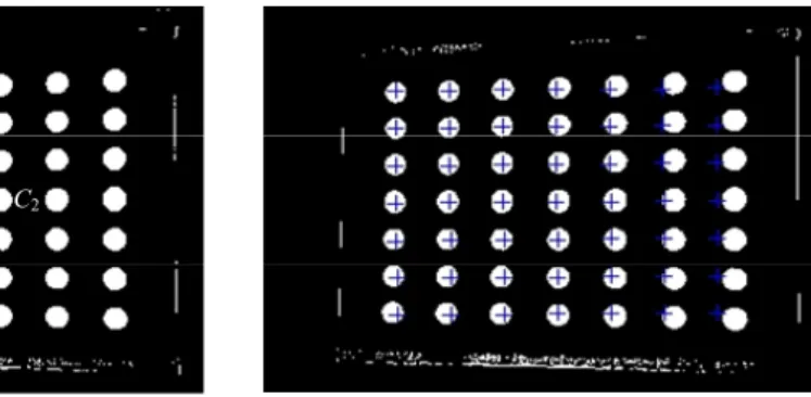
First, the grayscale image Gg of the dot-matrix pattern (for example, see Fig. 4 (c)) is thresholded into a binary dot-matrix pattern image Gb by Eq. (2). Fig. 4 (e) illustrates an example of the result. Then, a connected-component analysis algorithm is applied to Gb to extract the connected components in Gb. Some constraints on the component area, the ratio of the component width to the height, etc. are used to filter out unwanted noise. The result-ing connected components are white dots, denoted as CCi, i = 0, 1, …, n − 1, in the sequel. (b.2) Finding a cross-shaped group of five white dots near image center
Then we try to find a group of five white dots which form a five-dot cross shape near the center of Gb. The white dot nearest to the center Gb is first selected and denoted as C0. The nearest dot obtained by searching upward from C0 is selected next and
de-noted as C3. In the same way, the nearest dot obtained by searching downward from C0 is
denoted as C4. We also do leftward and rightward searches similarly and the results are
denoted as C1 and C2, respectively. See Fig. 8 for an illustration.
Next, we want to construct a cross-matrix pattern (CMP) from the binary dot-matrix P1 P3 P2' L1' L2' G1 G2 Ei = G1 - G2 Best fit Search window P2
pattern image Gb. The CMP has N × N crosses, with each cross “+” being located at a dot center. For this purpose, we first constructed a rough CMP with their crosses evenly dis-tributed horizontally and vertically with equal distances. An example constructed from Fig. 8 can be seen in Fig. 9. The horizontal distance Wg and the vertical one Hg between every two crosses are computed respectively as the averages of the halves of the width and the height of the five-dot cross shape obtained previously, i.e., Wg and Hg are com-puted as
Wg = (|C1 − C0| + |C2 − C0|)/2; Hg = (|C3 − C0| + |C4 − C0|)/2, (3)
where | ⋅ | represents the distance between two white dots.
C1 C0 C2
C3
C4
Fig. 8. A 5-dot cross shape near the center of
binary dot-matrix pattern image.
Fig. 9. Rough CMP superimposed on the binary dot matrix pattern image.
(b.3) Fine tuning of positions of crosses in rough CMP to obtain desired CMP
The crosses in the rough CMP are not located at the real centers of the white dots. See Fig. 9 for this phenomenon. But they can be used as the start positions for finding more accurate dot center locations. For this purpose, the rough CMP is first superim-posed on the dot-matrix pattern image Gg with the center of the five-dot cross shape overlapping on the center of Gg, or equivalently, on the center of CC0. Then, we use the
deformable template matching (DTM) method [8, 9] to do the fine tuning work of find-ing more accurate dot centers.
A deformable template DT for circular region detection as shown in Fig. 10 (b) with the parameters of its center (xi, yi) and radius ri is used to detect each white dot in the dot-matrix image Gg. The detection is started from the position of the cross of a white dot CCj in the rough CMP. And a search range, denoted as SR, is defined for the search of a best-match of the template DT with a desired dot. The width and the height of SR are defined to be the values of Wg and Hg defined in Eq. (3), respectively. SR is centered at a
position in Gg corresponding to the center of a cross in Gb. See Fig. 10 (a) for an illustra-tion. At every search point (k, l) defined by a position (xk yk), denoted as SPk, in the search range SR for a radius rl of the template DT, the edge values of the eight search windows around the circle of the DT are computed and summed up as the edge energy of the search point (k, l). The best-match search point with the maximum edge energy is found after all search points are tried, and the corresponding SPmax at location (xmax, ymax)
Wg Hg CCj SR (xi, yi) ri
(a) SR and CCj. (b) Circular template with 8 scan windows.
Fig. 10 Deformable template matching.
P6 P0 L6 L7 Li Ci1 Ci2 Pi Pi P7 Ci1 C i2 Li
Fig. 11 Extracting landmark point Pi at left side.
is taken to be the desired center position for the white dot CCj. A cross “+” is then drawn at (xmax, ymax). We do the same process for all the other dots, and this completes the
con-struction of the desired CMP. Fig. 4 (f) shows an example of the final results of applying this process.
(c) Extraction of extended dot centers on screen border
So far, we have obtained a CMP which includes accurate position information of the original dot centers, and an approximating polygon of the screen border. We need further the positions of the extended dot centers on the screen border. These positions can be calculated from the geometric information mentioned above. We describe the details below.
Referring to Fig. 11, an extended dot center point Pi on the left-hand side of the screen border can be extracted by utilizing the position information of the first and the second dots CCi1 and CCi2 on the ith row of the dot matrix. First, we obtain the line Li which connects the centers of CCi1 and CCi2 and extend it to the left-hand side. If the line Li is above vertex P7 of the polygon, then we compute the intersection point of Li with the polygon side L7; otherwise, we do so with the polygon side L6. The result is an
ex-Fig. 12. Calculating screen coordinates (Xi, Yj) in a basic region Rj and in border area Rg. tended dot center point Pi. We do similar works to obtain all the other extended dot cen-ters. The details are omitted. In Fig. 4 (f), the points marked with crosses “+” on the screen border are the extraction results.
2.3 Coordinate Transformation from Image Coordinates to Screen Coordinates After all the original and the extended dot centers are extracted, they form an (N + 2) × (N + 2) dot center matrix. For each of the dot center points, denoted by DPi, let its screen coordinates be denoted by (Xi, Yi) and its corresponding image coordinates by (xi, yi) where i = 0, 1, …, (N + 2) × (N + 2) − 1. The (N + 2) × (N + 2) points divide the field of view (FOV) (i.e., the full image) into (N + 3) × (N + 3) basic regions BRi, which con-sists of two portions: (1) the (N + 1) × (N + 1) inner basic regions inside the display screen, together forming a rectangular region called display area, denoted by Rdisplay, and
(2) the other basic regions between the border of the display screen and the outer border of the FOV, together forming a round region called border area, denoted by Rborder.
The last step of the desired calibration is a process of coordinate transformation from the image coordinates to the screen coordinates. The detail of the transformation, which is based on the concept of inverse distance weighting interpolation (IDWI), is de-scribed in the following.
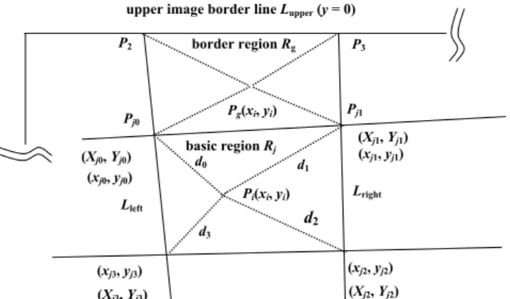
Referring to Fig. 12, let image point Pi with coordinates (xi, yi) be located within one basic region Rj of the display area Rdisplay and let the image and screen coordinates of the four corner points (i.e., four dot center points) Pj0, Pj1, Pj2, and Pj3 of Rj be (xjk, yjk) and (Xjk, Yjk), respectively, where k = 0, 1, 2, 3. Let the distance between image points Pi and Pjk be denoted as dk. We use the IDWI method to calculate the corresponding screen co-ordinates (Xi, Yi) of Pi as follows, where wk denotes 1/dk and W denotes the sum of w0
through w3 (i.e., W = w0 + w1 + w2 + w3): Xj = (Xj0 × w0 + Xj1 × w1 + Xj2 × w2 + Xj3 × w3)/W, (4) Yj = (Yj0 × w0 + Yj1 × w1 + Yj2 × w2 + Yj3 × w3)/W. (5) Pi(xi, yi) (xj1, yj1) (xj0, yj0) (xj2, yj2) (xj3, yj3) (Xj1, Yj1) (Xj0, Yj0) (Xj2, Yj2) (Xj3, Yj3) d0 d1 d2 d3 basic region Rj Pg(xi, yi) P3 Pj1 P2 Pj0 Lright Lleft border region Rg
It is noted that the screen coordinates (Xjk Yjk) are assumed to be known in advance. When a given image point Pi is outside Rdisplay and in Rborder, referring to Rg of Fig. 12 for example, we do not have a confining basic region like Rj above to enclose Pi. We have to create such an enclosing region for the above IDWI method to be applicable. For this, using the case illustrated by Fig. 12 as an example, let the basic region below Pg be Rj as mentioned above with Lleft and Lright as its two vertical side lines and Pj0 and Pj1 as its two upper corner points. Then we compute the intersection points of Lleft and Lright
with the upper image border line Lupper (with equation y = 0) and let the results be
de-noted as P2 and P3, respectively. Then, with Pj0, Pj1, P2, and P3 as the corner points of a
new basic region Rg, we can apply an IDWI process similar to the above-mentioned one to compute the corresponding screen coordinates for the image point Pg.
3. EXPERIMENTAL RESULTS
In this section, we show some experimental results of coordinate transformations from image coordinates to display screen coordinates by two different calibration meth-ods. One is the proposed method and the other a method proposed by Tsai [6]. The landmark points used in these two methods were extracted from an identical image of calibration patterns. The only difference is the way adopted to do the coordinate trans-formation. First, we briefly describe Tsai’s plane-to-plane calibration method which was implemented in this experiment. Then, we show the results of the two methods using the identical set of image points.
3.1 Plane-to-Plane Calibration by Tsai [6]
Assume that the landmark points in the world space (for our case here, on the planar display screen) are (Xi, Yi, Zi), i = 0, 1, …, N, with Zi = 0, and their corresponding image feature points are (ui, vi). The relationship between (ui, vi) and (Xi, Yi, Zi) can be described by the following equations:
( / ), ( / ) i i x y s s w h S pixel mm S pixel mm w h = = (7) , 2 2 i i x y w h C = C = (8) 2 2 2 , , i y i x d d d d x x y C x C u v r u v S S − − = = = + (9) 2 2 1 1 (1 ), (1 ) i d i d u =u +κ r v =v +κ r (10) , (perspective projection) i x i y u f v f z z = = (11)
(rigid body transformation)
i i i x X y R Y T z Z ⎡ ⎤ ⎡ ⎤ ⎢ ⎥= ⎢ ⎥+ ⎢ ⎥ ⎢ ⎥ ⎢ ⎥ ⎢ ⎥ ⎣ ⎦ ⎣ ⎦ (12)
where
11 12 13 21 22 23 31 32 33
cos cos sin cos sin
sin cos cos sin sin cos cos sin sin sin cos sin
sin sin cos sin cos cos sin sin sin cos cos cos
r r r R r r r r r r θ θ θ φ θ φ φ θ φ θ φ φ θ φ φ θ φ θ φ ⎡ ⎤ ⎢ ⎥ = ⎢ ⎥ ⎢ ⎥ ⎣ ⎦ Ψ Ψ − ⎡ ⎤ ⎢ ⎥ = −⎢ Ψ + Ψ Ψ + Ψ ⎥ ⎢ Ψ + Ψ − Ψ + Ψ ⎥ ⎣ ⎦ . x y z T T T T ⎡ ⎤ ⎢ ⎥ = ⎢ ⎥ ⎢ ⎥ ⎣ ⎦ (13)
In Eq. (7), (wi, hi) is the dimension of the image in the computer memory (640 × 480
pixel2 in this experiment), and (w
s, hs) is the physical dimension of the used CCD sensor
(3.2 × 2.4 mm2 in this experiment). In Eq. (8), (C
x, Cy) is the image center. In Eq. (9), (ud,
vd) specifies the distorted image point of (ui, vi) caused by optical imperfection. In Eq.
(10), κ1 is the radial distortion parameter of the camera lens. Here we assume that only
the first order distortion is considered. In Eq. (11), (ui, vi) is the perspective projection of (x, y, z) onto the image plane with the camera lens center of the camera as the origin of the camera coordinate system. In Eq. (12), (x, y, z) is the result of the coordinate trans-formation of (Xi, Yi, Zi) by rigid body rotation and translation specified by the rotation matrix R and the translation vector T. In Eq. (13), R and T are represented by detailed parameters.
With sufficient known landmark point pairs (ui, vi) and (Xi, Yi, Zi), we can use Tsai’s
method [6] to calculate all the parameters R, T and κ1. Then, we can use these parameters
to calculate the world coordinates (Xi, Yi, Zi) of any image point (ui, vi) to complete the coordinate transformation, as was done in our experiment.
3.2 Comparison of Results of Proposed Method and Tsai’s Method
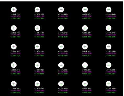
Referring to Fig. 4 again, we used calibration patterns Figs. 4 (a) through (c) to ex-tract landmark points which are marked in Fig. 4 (f) with “+.” These landmark points were used to conduct calibration both by the proposed method and by Tsai’s method as described previously. After the calibration process, the dot centers of the dot-matrix im-age were used to perform the coordinate transformation to get the coordinates of the dot centers in the display screen. Both results by using a 5 × 5 dot-matrix pattern for calibra-tion are showed in Figs. 13 and 14 for comparison. Fig. 13 shows the results using the set of the extracted image points which are identical to those used for calibration. Fig. 14 shows the results using a set of image points which were extracted from a new dot matrix pattern image. In the figures, the listed data r: <xxx, yyy> specify the real coordinates of the dot centers in the dot-matrix pattern, c: <xxx, yyy> specify the coordinate transforma-tion results using the proposed method, and t: <xxx, yyy> specify the coordinate trans-formation results using Tsai’s method.
Fig. 13. Comparison using calibration image points. The precise landmark position, the computed position by proposed method, and that by Tsai’s method are listed under each dot.
Fig. 14. Comparison using re-captured image points. The precise landmark position, the computed position by proposed method, and that by Tsai’s method are listed under each dot.
Observing Figs. 13 and 14, we can see that the coordinate transformation errors of Tsai’s method are larger than those of the proposed method, especially near the image border. In Fig. 13, we see that no coordinate transformation error was created by the proposed method. This is owing to the fact that the input image points used in the trans-formation are the same as those used in calibration. In Fig. 14, we can see some small coordinate transformation errors created by the proposed method. They were caused by
small image variations, leading toextraction of the dot centers at slightly different
posi-tions. But these errors are still smaller than those yielded by Tsai’s method.
4. CONCLUSIONS
A robust and accurate method for calibration and coordinate transformations from image coordinates to display screen positions has been proposed. By using three sequen-tially displayed calibration patterns, including a white-rectangle shape, a black-rectangle shape, and a dot matrix, relevant landmark points can be extracted accurately and robus-tly for calibration. Deformable pattern matching is used for creating more accurate geo-metric models for the display screen shapes in acquired images. The transformation of the coordinates of a point in the image to the coordinates of the display screen is done by using an inverse distance weighting interpolation method. Comparing the results with a conventional calibration method, we showed that the proposed method has the merits of more accuracy, robustness, and simplicity.
REFERENCES
1. K. Hansen and C. Stillman, “Computer presentation system and method with optical
tracking of wireless pointer,” US Patent, No. US6275214.
2. S. H. Lin, “Interactive display presentation system,” US Patent, No. US6346933.
3. L. S. Smoot, “Light-pen system for projected images,” US Patent, No. US5115230.
4. D. R. Olsen and T. Nielsen, “Laser pointer interaction,” in Proceedings of
Con-ference on Human Factors in Computing Systems, 2001, pp. 17-22.
5. C. Kirstein and H. Müller, “Interaction with a projection screen using a camera-
tracked laser pointer,” in Proceedings of International Conference on Multimedia
Modeling, 1998, pp. 191-192.
6. R. Y. Tsai, “An efficient and accurate camera calibration technique for 3D machine
vision,” in Proceedings of IEEE Conference on Computer Vision and Pattern
Rec-ognition, 1986, pp. 364-374.
7. J. Salvi, X. Armangué, and J. Batle, “A comparative review of camera calibrating
methods with accuracy evaluation,” Pattern Recognition, Vol. 35, 2002, pp. 1617- 1635.
8. K. L. Tam, R. W. H. Lau, and C. W. Ngo, “Deformable geometry model matching
by topological and geometric signatures,” in Proceedings of the 17th International
Conference on Pattern Recognition, Vol. 3, 2004, pp. 910-913.
9. A. L. Yuille, P. W. Hallinan, and D. S. Cohen, “Feature extraction from faces using
deformable templates,” International Journal of Computer Vision, Vol. 8, 1992, pp. 99-111.
10. R. Sukthankar, R. G. Stockton, and M. D. Mullin, “Smarter presentations: exploiting homography in camera-projector systems,” in Proceedings of International
Confer-ence on Computer Vision, Vol. 1, 2001, pp. 247-253.
Sheng-Wen Jeng (鄭勝文) received the B.S. degree in Electronics Engineering
from National Chiao Tung University in 1983, the M.S. degree in Electro-optical Engi-neering from National Chiao Tung University in 1985. Mr. Jeng worked as a researcher in the Industrial Technology Research Institute since October 1985 till now. He is also a Ph.D. student in the Department of Computer Science at National Chiao Tung University since 1997. His current research interests include computer vision, pattern recognition, MEMS, and their applications.
Wen-Hsiang Tsai (蔡文祥) received the B.S. degree in Electrical Engineering from National Taiwan University in 1973, the M.S. degree in Electrical Engineering from Brown University in 1977, and the Ph.D. degree in Electrical Engineering from Purdue University in 1979. Dr. Tsai joined the faculty of National Chiao Tung University (NCTU) in Taiwan in November, 1979, and was an NCTU Chair Professor in the De-partment of Computer Science. Since August, 2004, he has been the President of Asia University in Taiwan.
At NCTU, Professor Tsai was the Head of the Department of Computer and Infor-mation Science from 1984 to 1988, the Dean of General Affairs from 1995 to 1996, the Dean of Academic Affairs from 1999 to 2001, and Vice President from 2001 to 2004. He served as the Chairman of the Chinese Image Processing and Pattern Recognition Soci-ety of Taiwan from 1999 to 2000. He has been the Editor of several academic journals, including Journal of the Chinese Engineers, International Journal of Pattern Recognition and Artificial Intelligence, Journal of Information Science and Engineering, and Pattern Recognition. He was the Editor-in-Chief of Journal of Information Science and Engi-neering from 1998 to 2000. Professor Tsai’s major research interests include image proc-essing, pattern recognition, computer vision, virtual reality, and information copyright and security protection. Dr. Tsai is a senior member of IEEE and is currently the Chair of the Computer Society of IEEE Taipei Section in Taiwan.