以失真為基礎的車際網路影像串流傳輸機制

國

立

交

通

大

學

網路工程研究所

碩

士

論

文

以失真為基礎的車際網路影像串流傳輸機制

Distortion-based Video Streaming over

Vehicular Ad Hoc Networks

研 究 生：孫冠宇

指導教授：陳 健 教授

以失真為基礎的車際網路影像串流傳輸機制

Distortion-based Video Streaming over

Vehicular Ad Hoc Networks

研 究 生：孫冠宇 Student：Kuan-Yu Sun

指導教授：陳 健 Advisor：Chien Chen

國 立 交 通 大 學

網 路 工 程 研 究 所

碩 士 論 文

A Thesis

Submitted to Institute of Network Engineering College of Computer Science

National Chiao Tung University in partial Fulfillment of the Requirements

for the Degree of Master

in

Computer Science

June 2011

Hsinchu, Taiwan, Republic of China

以失真為基礎的車際網路影像串流傳輸機制

學生：孫冠宇

指導教授：陳健 教授

國 立 交 通 大 學 網 路 工 程 所

中文摘要

雖然至今為止已有許多針對 VANET 特性及需求而提出的路由協定，但是大 部分的這些研究工作並不適合用來傳遞即時影像串流。因為 VANET 非常容易因 為車輛的行駛行為而造成網路局部性的斷線以及整個網路拓樸的改變。這些與生 俱來的天性使得許多現有的路由協定很難能夠滿足影像串流或是其它多媒體相 關的應用對於封包延遲時間的要求。為了解決這樣的問題，本論文提出了一個基 於交通統計資訊以及影像失真程度的路由協定。這個協定主要是透過將每條道路 路段指定一個估計的失真數值以作為該路段是否適合用來傳遞影像封包的權重， 然後我們可以據此找出最適合傳影像的路段組合。同時，本論文也提出一個應用 Markov Decision Process 的概念的封包傳遞機制，來幫助持有影像封包的車輛找 出下一個適合的封包轉傳車輛。在此我們採用 NS2 網路模擬器來評估我們演算 法的效能，模擬結果顯示出我們的方法的確能讓使用者獲得更佳的視訊品質。

Distortion-based Video Streaming over

Vehicular Ad Hoc Networks

Student: Kuan-Yu Sun Advisor: Dr. Chien Chen

Institute of Network Engineering

National Chiao Tung University

Abstract

There are already many routing protocols tailored for Vehicular Ad Hoc Networks (VANET). However, most of them are not suitable for real-time video streaming. The frequently isolating network partitioning nature and constantly changing network topology of VANET makes it difficult for existing protocols to satisfy the strict delay requirements of video streaming or other multimedia applications. To address this issue, this thesis proposes a routing protocol which considers both the traffic statistics information and possible video distortion to assign different weights to each road segment, and find the best path for video packet dissemination accordingly. This thesis also proposes a Markov Decision Process (MDP) based forwarding scheme for the process of packet delivery. The simulations are carried out by NS2 to validate the performance of our proposed protocol. The results show that the proposed solution can really yield good user perceived video quality.

Keywords: VANET, Routing Protocol, Video Streaming, Distortion, Markov Decision Process.

誌謝

“感謝主”，終於有個機會可以寫出這句話了！這篇論文是靠很多人長期的幫 助和關心之下才得以完成的。首先，我要感謝我的指導教授陳健博士，因為老師 長期悉心指點，不吝撥空與我討論，在我沒想法的時候仍給予鼓勵，指導我做事 情應有的態度。這篇論文的完成，也要感謝我的口試委員們：簡榮宏教授、陳志 成教授、張適宇教授，謝謝他們百忙中撥冗參與口試，並對我的論文內容提供寶 貴意見。 感謝我的學長陳盈羽、張哲維與陳坤定，在我撰寫論文方面提供各樣協助。 特別是哲維學長，花了許多時間和我討論，提供我想法，使得這篇論文的內容才 能夠成形。感謝我的同學莊敬中與黃鼎峰，謝謝他們長期支持我和罩我，讓我的 研究所生涯多了很多值得回味的故事。感謝我的學弟們：王柏翔、彭宣翰、鄭元 碩、張大鈞、蔡世仁、蔡沛勳和黃俊憲，陪我渡過種種歡笑與煩悶。 再來我想感謝交大學園團契的輔導們和同學們，謝謝他們這幾年來有聲無聲 的關心。感謝交大研究生團契的應數系陳福祥教授、王國仲教授與研究生們，提 供我一個心靈的出口。感謝 Raghavendra M. Kulkarni，使我在英文方面受教不少。 感謝老室友陳耿賢和秦健候，讓我有難忘的宿舍生活和西提牛排招待。感謝幫助 過我當家教的陳阿姨一家人，把我當作她們的一份子。感謝電資學士班的助理惠 婷姊，對後輩的照顧不餘遺力。感謝當初一起考研究所的朋友劉冠麟和張龍盛， 與我一同並肩作戰。感謝華岡團契的諸位，對我多年來的關心。還有很多沒感謝 到的人，他們的付出我會一直感念於心。 最後，我想特別謝謝愛我的父親、母親和老弟，他們永遠都是我精神上的力 量，是這一路上最信任最包容我的人。父母含辛茹苦地養育我，教我做人處事的 道理，恩惠之深，我無以為報，在此謹獻上最深的感謝。

Table of Content

中文摘要... i Abstract ... ii 誌謝... iii Table of Content ... iv List of Figure ... v List of Table ... vi Chapter 1: Introduction ... 1

Chapter 2: Related Works ... 4

2.1. VADD ... 4

2.2. VANET routings for video streaming ... 4

2.3. Distortion-based video streaming in MANET ... 6

Chapter 3: Proposed Algorithm ... 9

3.1. Algorithm description ... 9

3.2. Shadowing propagation model ... 10

3.3. Distortion assessment for a specific road segment... 12

3.4. MDP-based forwarding scheme ... 26

3.5. Other protocol operations ... 30

3.6. An implementation paradigm for urban scenarios ... 31

Chapter 4: Simulation ... 32

4.1. Validating the proposed distortion calculation approach ... 32

4.2. Performance evaluation for the proposed routing algorithm ... 37

Chapter 5: Conclusion ... 45

List of Figures

Figure 1: The concept of the proposed algorithm. ... 9

Figure 2: The transmission ranges of shadowing model and the deterministic propagation model. ... 11

Figure 3: The packet error rate under shadowing model. ... 12

Figure 4: A model used for hop-by-hop distortion calculation. ... 13

Figure 5: Illustration of the scenario used for the packet collision probability calculation. ... 15

Figure 6: The space coverage of the RTS frame and the CTS frame... 16

Figure 7: The retransmission scheme of IEEE 802.11 DCF. ... 17

Figure 8: Possible contention window size by applying binary exponential backoff algorithm. ... 19

Figure 9: The average distance to each neighbor vehicle in transmission range. ... 25

Figure 10: An example of total packet dropping probability ... 25

Figure 11: The forwarding scenario without the need of MDP operations ... 26

Figure 12: Illustration how to map the cells of the road segment to a series of states. 27 Figure 13: The 4 concerned actions in this study. ... 28

Figure 14: Illustration of the initial distortion calculation approach for value iteration. ... 30

Figure 15: MAC error probability vs. hop distance. ... 34

Figure 16: Average service time vs. hop distance. ... 35

Figure 17: Average packet sojourn time vs. hop distance. ... 36

Figure 18: PSNR vs. hop distance. ... 37

Figure 19: The used highway scenario. ... 38

Figure 20: PSNR results of different road density and road segment length under 0.3 second video deadline. ... 39

Figure 21: PSNR results of different video deadline under the medium density. ... 40

Figure 22: PSNR results of different forwarding schemes. ... 42

List of Tables

TABLE I: Parameters used in ns2 simulator. ... 33 TABLE II: Parameters used for algorithm evaluation. ... 38

Chapter 1: Introduction

Vehicular ad hoc networks, a type of Mobile Ad Hoc Networks (MANET), build wireless networks between vehicles and road side units to potentially provide safer driving experiences and many useful non-safety applications. To deploy this emerging technology in real life, governments, automobile industries, and academic research community have paid considerable attention over recent years. Moreover, the 75 MHz of spectrum in the 5.9 GHz band has been delegated as Dedicated Short Range Communication (DSRC) by the U.S. Federal Communications Commission (FCC) in 1999 [1]. On the other hand, for the process of protocol standardization, the IEEE 802.11p and IEEE 1609 series of standards are also proposed by IEEE to address this requirement [2][3].

Also, many existing VANET routing research results [4][5] have demonstrated that the unique characteristics of road traffic environment make the conventional MANET routing protocols, such as AODV, DSR, and GPSR, inefficient and unproductive. Several researchers have also presented diverse routing paradigms to improve the performance of information distribution by taking the characteristics of the traffic environment and road structure into account. Among the prior research efforts, VADD [6] looked at both the traffic statistics information and the topology of the local road map to construct a packet delivery path with minimum possible delivery delay.

Unlike normal data transmission, video streaming could let drivers include more suitable applications for human cognitions: (1) providing driver assistance and navigation by collecting and displaying the surrounding view to help drivers make better driving decisions (2) enabling video conferencing/conversation between passengers of different vehicles (3) video surveillance [7] helps a country’s

transportation department to monitor the road traffic regulations (4) video advertising can be integrated with location-based services by local stores to offer advertisements to nearby vehicles (5) entertainment applications such as games [8][9], movies, and shows may also serve as feasible means for relaxing passengers during long distance travel. However, streaming video over VANET presents many challenges about the problems caused due to characteristics of wireless vehicular networks and video streaming. First of all, the rapidly-changing network topology and relatively higher vehicular mobility not only frequently breaks the network connections, but also makes a huge negative impact on network maintenance. Second, the strict video decoding deadline constraint is not easy to satisfy if the quality of the network is unstable. In addition, the bursty traffic, larger packet size, and variable bit rate (VBR) transmission nature of video streaming are also difficulties which make the challenges of video delivery even hard to overcome and solve. In spite of the aforementioned difficulties, [10] and [11] indicate the advancement of wireless networks and video compression technologies, thus making the non-trivial idea of video streaming over VANET a reality. The emerging IEEE 802.11p can support data transfer rates up to 54 Mbps between vehicles and road side wireless infrastructures. Next, the multi-channel communication ability of IEEE 802.11p greatly improves the attainable throughput by adding the frequency diversity. Lastly, the H.264/SVC introduces time, space, and quality scalability, and significantly increases the video coding efficiency [12], and therefore this technology is a good choice to alleviate the effects of the error-prone channels [11].

In MANET routing, research efforts about video streaming have already gathered some momentum. We noted that more and more researchers related to this topic have been changing the considered metrics from network-centric factors to

jitter and network bandwidth, the metrics concerned with classical MANET routing protocols; and the latter is about the user received video quality, which is more suitable for the streaming problem. According to [12], the multimedia-centric routing protocols typically utilize a cross-layer design approach while the network layer protocols make use of the application layer metrics.

In the works of [13][14][15], the authors proposed routing algorithms for wireless ad hoc networks, by considering the possible video distortion to find the optimal routing path to deliver video streaming. According to their works, we know the distortion may be caused by packet transmission error and video deadline expiration. The probabilities for these events are calculated by simplified MAC retransmission assumptions and queuing theory. Their works inspired us to apply the concepts into our problem.

Based on the mentioned research, we come up with a solution to deliver video streaming over VANET no matter for urban or highway scenarios. We divide our algorithm into two stages: the first stage is to estimate the video distortion values for vicinity road segments based on some traffic statistics information (in other words, we guess the possible video distortion if the video packets pass through the specific road segment), and we can find the routing path with minimum distortion by Dijkstra’s shortest path algorithm; after getting the path plan, the second stage uses a Markov Decision Process (MDP) based forwarding scheme to find suitable neighbor as the next hop.

The remaining sections are organized as follows. Chapter 2 reviews related works. Chapter 3 demonstrates the proposed distortion estimation model and the MDP-based packet forwarding scheme. Finally, chapter 4 shows the simulation results and chapter 5 gives the conclusion of our work.

Chapter 2: Related Works

2.1. VADD

The high mobility of vehicles and the rapid-changed network topology result in the vehicular network disconnecting frequently. This occurs more easily when the vehicular density is sparsely (e.g., not rush hour).

VADD [6] targets at solving such problem by exploiting the opportunities of intermittent connection between moving vehicles. Different from connection-oriented routing protocols, such as AODV and DSR, VADD does not need the exchanges of routing control messages to establish a path with end-to-end connection, maintain the available paths and repair the broken path. Therefore, the routing cost can be significantly reduced. VADD utilizes the idea of carry-and-forward scheme which is well known in the area of Delay Tolerance Networks (DTN), to pass packets while the network connection is unserviceable. A sender vehicle can just carry the unforwardable packets until it meets other vehicles in transmission range, and relays the buffered packets to those neighboring vehicles. This is of great help to delay-tolerant applications.

By the traffic statistics information provided from the preloaded digital maps and by the coordinates obtained from the GPS device, a stochastic delay model is built accordingly. The delay model estimates the data-delivery delays to assist the road segment (or intersection) selection, and finds the minimum delivery delay path further.

2.2. VANET routings for video streaming

The authors of V3 [10] provided a vehicle-to-vehicle live video streaming architecture for highway scenarios. Vehicles in the destination region act as video

sources to capture and send the videos which contain the surrounding information to the requester vehicles. To accomplish this goal, a video source trigger sub-system and a video data transfer sub-system are proposed as the main functionalities of V3. The former uses a signaling mechanism to let the requester vehicles can possess the freshest video information by continuously triggering the video sources to send video back; and the latter applied the carry-and-forward scheme to efficiently transfer video packets by using some forwarder selection approaches. However, the authors did not use real video data in the simulation.

[16] also proposed two routing protocols, the sender-based forwarding (SBF) and receiver-based forwarding (RBF), to send video packets in highway environment. SBF chooses the vehicle which is closest to the destination vehicle to be the packet forwarder, this approach is also known as greedy forwarding. In addition, RBF follows the concept of contention-based forwarding [17] to elect forwarders. The sender vehicles apply broadcast to transmit video packets instead of unicast. The neighboring vehicles which have received the packet will delay a short period before sending to the link layer according to the delay principle. If the node with shortest delay has broadcasted the packet out, then other nodes overhearing the transmission will discard the packet. According to their work, we can observe that the RBF approach has no need of any control packets and achieves better performance than SBF because of no extra overhead. Nevertheless, [18] indicated the delay time should be large enough to distinguish the best forwarding candidate and other candidates. Furthermore, the delay time should be short to avoid unnecessary waiting time. How to design a delay function which is suitable for the traffic with bursty nature is not trivial.

For the urban environment, [19] proposed a cross-layer path selection algorithm to send video packets with the help of road side units (RSUs). The authors adopted a

stochastic mobility model which divides a road segment into the front, the middle and the end parts to consider, and queuing theory was used to calculate the connectivity of a road segment. The RSU plays a role of the video source; it sends packets to the destination vehicle via the relaying of moving vehicles. Vehicles periodically broadcast their location information and the RSU can accordingly plan a best routing path to deliver video packet by using video distortion as the concerned routing metric. Different to this work, the study of this thesis does not rely on the help of RSUs, we try to follow the similar way of VADD to deliver video packets.

2.3. Distortion-based video streaming in MANET

To provide better video streaming services in mobile computing devices and wireless networks, researchers start to consider the relationship between the characteristics of the video and of the wireless network environment in their research. Such researches aim at offering the end users better perceived video quality. Because the video quality perceived by each user is probably not the same, Peak Signal-to-Noise Ratio (PSNR), the most widely used metric to measure the quality of received video, can helpfully judge the quality of video:

(1)

and the Minimum Square Error (MSE) is:

(2)

The purpose of PSNR is to measure the difference between the original video frame and the processed video frame. The higher PSNR value, the better video quality, and vice versa.

Stuhlmuller, et al. [20] provided an empirical rate-distortion model for a hybrid motion compensated video encoder. The authors analysis the codec structure of H.26x

and MEPG-x series video coding standards to induce the general form of rate-distortion model. The model is

(3)

where , and are distortions with respect to decoder side, encoder side and network transmission; , , and are encoder related parameters. The distortions are in the form of MSE and can be converted to PSNR values by

(4) In this study we only focus on how to calculate (the distortion caused by network transmission). The value of is mainly represented in the form

_{, where is a constant related to the video sequence structure and the codec} features, which describes the distortion if a video packet cannot be decoded successfully. is the packet dropping probability which is decided by the

characteristics of applied radio propagation model.

[13] proposed a distortion-based routing path selection algorithm for static ad hoc networks. The work applied the rate-distortion model as mentioned earlier, and focused on how to calculate the . According to their research, the packet

dropping probability can be divided into two parts: (1) the packet drop due to transmission error (by radio fading or MAC dropping scheme) and (2) due to

video packet deadline expiration . Thus, as shown in equation (5), the can

be re-expressed as the sum of the distortions caused by transmission error

and the deadline expiration , respectively.

(5)

The routing algorithm proposed by [14] and [15] considers not only the channel and packet expiration issues but also the influences of the video encoding parameters. They based upon the factors to find an optimal routing path for individual packets. The distortion calculation approaches are basically similar to [13] (although the used distortion models are different).

Chapter 3: Proposed Algorithm

3.1. Algorithm description

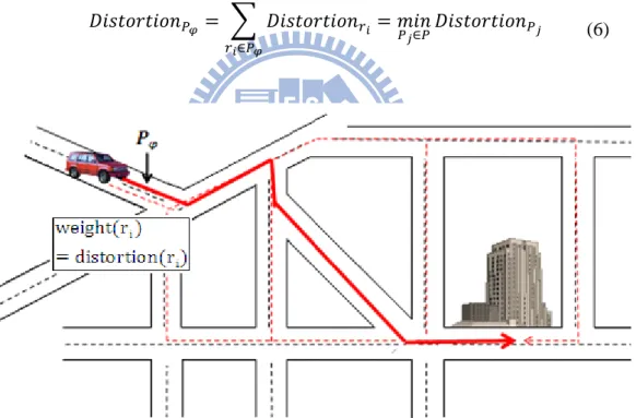
The road network is considered as an undirected graph , where is the set of intersections, and is the set of road segments. The video will be distorted by if the video stream passes through the road segment . Then we want to find a path which leads to minimum video distortion, from the entire possible road paths set between the source vehicle to a given fixed location (e.g., a gas station, a restaurant or an office building). That is:

(6)

Figure 1: The concept of the proposed algorithm.

All vehicles are assumed to be equipped with faultless GPS devices which thereby help in finding their current positions. Moreover, the digital maps are assumed to be pre-loaded in each vehicle, thus it is able to obtain the road structures, and some traffic statistics information such as the length and the vehicular density of the road

segment. Based on these assumptions, we define the distortion value for each road segment by using the traffic statistics contained in the digital map. Then the Dijkstra’s shortest path algorithm is applied to find out the video delivery path with minimum video distortion. Although we can refer the traffic statistics to estimate the video distortion for a specific road segment and the corresponding hop length, but in fact the actual vehicle placement possibly is not in the ideal placement; moreover, the various nearby forwarding vehicles of a sender cause different distortions. For this reason, a MDP-based forwarding scheme is further proposed by considering the estimated distortion information.

3.2. Shadowing propagation model

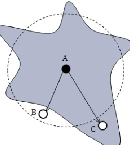
To demonstrate the real world behavior of radio waves, we employ the shadowing model to represent a practical physical layer. The predicted received power by free-space model and two-ray ground model are deterministic functions of distance, so the transmission range is considered to be an ideal circle [21]. Shadowing propagation model takes the multipath propagation effects into account to add randomness to the predicted received power. As depicted in Figure 2, the curve of the gray area indicates the possible transmission range of shadowing model; the dashed line indicates the transmission range of the deterministic model.

The shadowing model is represented as

(7)

where and are received powers at certain distance and reference distance , is the path loss exponent, is a Gaussian random variable with zero mean and standard deviation .

Figure 2: The transmission ranges of shadowing model and the deterministic propagation model.

In the implementation of ns2 [21], a packet can be received only if the received power is greater than a specific receiver threshold . Based on the implementation, we can calculate the average packet error rate for a given distance under ns2. The reference power is calculated by using the free-space model

(8)

where Pt is the transmitted power. Gt and Gr are the antenna gains of the transmitter

and the receiver respectively. λ is the wavelength and L is the system loss. The average path loss is

₍₉₎

and the average received power is

(10) Finally the following formula can be used to calculate the average packet error rate [22]

(11)

₍₁₂₎

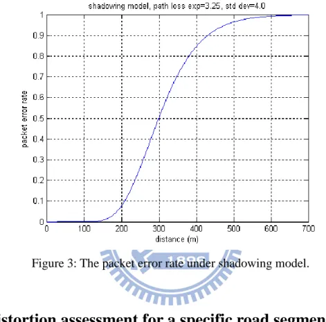
We plot the packet error rate with path loss exponent as 3.25 and shadowing deviation as 4.0 as Figure 3. The transmission range here is defined as 300m with packet error rate as 0.5.

Figure 3: The packet error rate under shadowing model.

3.3. Distortion assessment for a specific road segment

To discover whether a road segment is vital for video packet delivery in the proposed algorithm or not, depends on the possible video distortion created. The goal is to find a road path which leads to the minimum video distortion to deliver video packets.

Considering the nature of VANET, the possibility of network disconnection may be caused by the dynamics of vehicles and the unexpected driving behaviors. Although researchers have adopted the idea of carry-and-forward to handle this unpleasant situation, the strict packet delivery deadline requirement makes this approach not really work well in video streaming. Therefore we modified the rate-distortion

formula mentioned above to add this impact in: (13)

where is the distortion led by network disconnection, and is the

corresponding packet dropping probability (because there is no route at that moment).

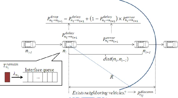
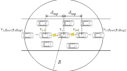
Figure 4: A model used for hop-by-hop distortion calculation.

The scenario of video packet delivery could be expressed as Figure 4. is the expiration probability due to the queuing delay at vehicle ni, and

_{is the}

packet dropping probability between vehicle ni and vehicle ni+1 caused by failed MAC

retransmissions. We combine and to stand for the overall packet dropping probability when the network is connected, and denote it as

₍₁₄₎

and are the packet arrival rate and remaining available time of the

consider the probability of the road connectivity for road segment based on the traffic statistics. We then calculate the video distortion for a given road segment by the model.

3.3.1. Probability of road connectivity

According to [6], [23] and [24], we assume the inter-vehicle distance follows an exponential distribution. If the average vehicular density is for the road segment

, then the disconnected probability is

₍₁₅₎

where is the road length, and the value of shows the number of hops needed to pass through . Although the transmission range and the packet receiving

probability of shadowing model are variables, we still use to estimate the connectivity of a road segment for simplicity.

3.3.2. Probability of MAC retransmission error

This study computes the packet failure probability by two factors: radio fading and packet collision. Given an inter-vehicle distance d, the packet error probability from radio fading is derived from equation (11). To calculate the packet collision probability, a simplified scenario as depicted in Figure 5. Suppose that vi is

the current video sender, vi-1, vi-2, …, are the predecessor senders, and vi+1,

vi+2…, are the successor senders (i.e., white cars). The rest vehicles in vi’s

transmission range only broadcast HELLO messages periodically (i.e., red cars). Suppose the HELLO time interval is , then the corresponding frequency

is:

There are two conditions to cause the collision: (1) one of vi’s neighbor nodes

transmits during vi’s RTS period or (2) one of vi+1’s neighbor nodes transmits during

vi+1’s CTS period. This study assumes that a successfully RTS/CTS transaction can

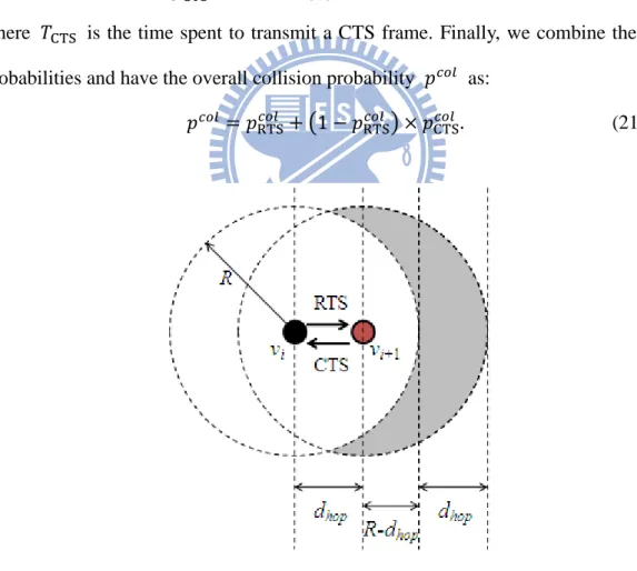
perfectly occupy the wireless channel, where no other vehicles can transmit packets during the channel occupation time. Therefore, for vehicle vi+1, only the neighbor

nodes of vi+1 outside vi’s transmission range should be considered (i.e., the vehicles inside gray area in Fig.6). Based on above observation, the collision probabilities for a sending RTS frame and a responding CTS frame can be calculated accordingly.

Suppose that the packet arrivals in VANETs are Poisson distributions no matter for video packet or HELLO message. Given a vehicular density ρij and a hop distance

between any two sequential video sender vehicles, the accumulated packet

arrival rate from vi’s neighbor nodes can be derived as:

(17)

where is the video packet arrival rate. and are the number of

neighboring vehicles with and without video traffic respectively. Figure 5: Illustration of the scenario used for the packet collision probability calculation.

and . The collision probability for a sending RTS frame

is:

(18)

where is the time spent to transmit a RTS frame. We then calculate the collision

probability for a responding CTS frame according to Figure 6. The accumulated packet arrival rate is:

(19) and the collision probability is:

(20)

where is the time spent to transmit a CTS frame. Finally, we combine the two

probabilities and have the overall collision probability as:

(21)

Figure 6: The space coverage of the RTS frame and the CTS frame

(22)

and

(23)

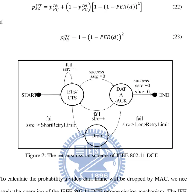
Figure 7: The retransmission scheme of IEEE 802.11 DCF.

To calculate the probability a video data frame will be dropped by MAC, we need to study the operation of the IEEE 802.11 DCF retransmission mechanism. The IEEE 802.11 DCF standard presents a retransmission approach, a frame must be transmitted successfully in a specific attempt limit or it will be discarded. Figure 7 shows the retransmission scheme. ssrc is known as Station Short Retry Count and slrc is known as Station Long Retry Count, they are with respect to the retry limits ShortRetryLimit and LongRetryLimit. ssrc is for the frames which are less than or equal to the

RTSThreshold, and slrc is for the frames which are longer than the RTSThreshold.

Every time a RTS/CTS transaction failure is occurred, the ssrc is increased by 1, and a DATA/ACK transaction failure will increase the slrc by 1. The increment of the contention window size is caused from both transaction failures. If a RTS/CTS transaction can be completed successfully, then the ssrc will be reset to 0. In the same

way, successful DATA/ACK transaction also let the slrc be reset to 0. Frames will be dropped if then ssrc exceeds the ShortRetryLimit or the slrc exceeds the

LongRetryLimit.

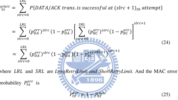
So we can calculate the probability that the video packet can be sent out

successfully by taking such retransmission scheme into account. After applying conditional probability, we have:

(24)

where and are LongRetryLimit and ShortRetryLimit. And the MAC error probability is

(25)

3.3.3. Probability of packet deadline expiration

In this subsection, the probability of packet deadline expiration will be investigated. That is, the possibility the packet sojourn time at a vehicle will exceed the remaining available time. The first step here is to calculate the packet service time. To estimate the service time adequately, the impacts from binary exponential backoff (BEB) is considered.

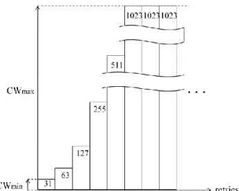
Figure 8 depicts the BEB algorithm, every time a packet cannot be transmitted successfully, the current backoff stage of the station node will be increased by 1, and its contention window (CW) size will be doubled until the window size reaches the . The contention window size will be reset to only if the MAC decides

Figure 8: Possible contention window size by applying binary exponential backoff algorithm.

to discard the packet or the packet can be successfully sent out. The following equation can be used to compute the contention window size:

(26)

where is the current backoff stage and is the maximum backoff stage. Between two consecutive contention window decrements, the time interval, which can be formulated as the sum of a constant slot time Tslot and an extra delay time E[Tfreeze]

caused by the surrounding packet transmission [33].

(27)

is the probability if there is at least one neighboring vehicle transmits packet

during a single slot time, this could be derived by applying the simplified scenario shown as Figure 5.

(28)

where

_{. In addition, p}

s is the probability that a

transmitting neighboring vehicle can finish the packet transmission during a slot time period without any contending transmissions simultaneously:

(29)

For T1 to T4, the calculations can be found in [33], as:

(30) where , , and stand for the frame transmission time of RTS,

CTS, DATA and ACK, respectively. and are the time

needed to discover the transmission failures for RTS/CTS transaction and DATA/ACK transaction. In this thesis, and are set as the

same as and , to match the ns2’s implementation [21].

In the proposed approach, the service time is divided into 3 parts to analysis: (1) time for successful transmission ; (2) time for unsuccessful RTS/CTS

transmission ; (3) time for unsuccessful DATA/ACK transmission .

By considering all the possible retransmission cases, the average service time for successful transmission is derived as follow:

(31) where and (we ignore the effects of propagation delay). is the spent time for a given retransmission case which sums up the time cost of random backoffs, RTS/CTS handshakes and DATA/ACK handshakes:

(32)

In equation (31), we notice that the form of which can help us to reduce the equation representation. Considering the question: find the number of non-negative integer solutions for the equation

We know Inclusion-Exclusion Principle can be applied to solve the question. So the following function is defined to stand for the answer.

(33)

And therefore the can be rewritten as

In the same way we can derive the average service time for :

(35)

where follows the same idea as :

(36)

And the average service time for :

(37)

where is: (38)

Finally the overall average service time is

(39) After the derivation of the average service time, how to calculate the packet expiration probability is the point here. In the research of [13], [14] and [15], the authors all assumed the packet queues are M/G/1 queues that means the inter-packet arrival following Poisson distribution. In reality, the Poisson arrival assumption probably is not true. For example, a video frame comes at , and which is separated into packets according to the frame size, so the packet queue instantly has new packets; the next video frame may come at and makes the queue instantly have new packets, etc. However, for the computation simplicity, we still follow the M/G/1 assumption to calculate the packet expiration probability. By the Pollaczek-Khinchin (P-K) formula, the packet waiting time can be expressed as

(40)

where is the packet arrival rate at vehicle . Therefore, the average packet sojourn time and the packet expiration probability [13][14][15] can be calculated as:

and (42)

where is the remaining available time for a video packet at vehicle . The

packet dropping probability is (43)

And then the dropping probability can be used to calculate the packet arrival rate and the remaining available time for vehicle , as

and

.

By the above discussion, we know the distortion for a hop is . Consequently, the distortion for the whole road segment can be further expressed

as: (44)

where is the set of all possible hop lengths by considering the vehicle placement:

(45)

For the vehicle , if its best forwarder is just meters away from itself ( is the average inter-vehicle distance according to the average vehicular density for the road segment ), then we averagely think the best forwarder of the

vehicle should be also away from itself meters. If the best forwarder vehicle of the vehicle is meters away, two times of the average inter-vehicle distance by Gamma distribution, then we also think averagely the best

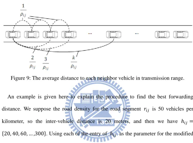
forwarder of the vehicle should be also away from itself meters. By analogy, after considering the average distance to each neighbor in transmission range, the distance which leads to minimum distortion will be picked. Figure 9 gives an illustration.

Figure 9: The average distance to each neighbor vehicle in transmission range.

An example is given here to explain the procedure to find the best forwarding distance. We suppose the road density for the road segment is 50 vehicles per

kilometer, so the inter-vehicle distance is 20 meters, and then we have

. Using each of the entry of as the parameter for the modified distortion model, the corresponding packet dropping probabilities for the entire road segment can be calculated as Figure 10.

Figure 10: An example of total packet dropping probability

160 meters, hence 160 meters will be designated in the distortion estimation, and treated as the best forwarding distance.

3.4. MDP-based forwarding scheme

At the stage of distortion calculation, the considered forwarding distance is

calculated based on the assumption of ideal vehicular placement. However, in the real road traffic scenario, there is probably having no neighbor vehicle just away from each vehicle . So the best forwarding distance is actually a reference to help us

find the suitable forwarder vehicle. Therefore we propose a MDP-based forwarding scheme to delivery video packets between moving vehicles. MDPs are stochastic processes used for modeling decision-making problems, the outcomes of which are partly under the control of the decision makers. This mathematic tool is very useful to solve the optimization problems. A MDP is consisted of a set of states, a set of actions and a set of rewards. After giving an object function, the MDP can find out the best action/decision by utilizing value-iteration or policy-iteration, the two well-known algorithms to solve MDPs [25].

There are two cases for the packet forwarding scheme:

 Case 1: Suppose there is a vehicle located in the expected region which is marked with a star in Figure 11 as shown below, and then we directly select it as the next forwarder.

 Case 2: If there is no vehicle located in the expected region, then we apply a Markov Decision Process to decide a forwarder selection policy.

Given a road segment or a road distance, we divide the distance into a number of cells, and each of the cells will be mapped to a corresponding state of the Markov chain, as shown in Figure 12.

Figure 12: Illustration how to map the cells of the road segment to a series of states.

Suppose the length of a cell is , then there are cells in a vehicle’s transmission range. We mark the cell the best forwarding distance is located; assign the highest priority to the specific cell, and different lower priorities to the remaining cells. Such a priority setting pattern is an action. One of the straightforward priority assignment methods is exhausted assignment which can surely cover all the possible cases, but the computational complexity is obviously substantial. For instance, there are possible actions for a vehicle. Because we already know which the best cell is, we can intuit the higher priority cells should be adjacent to the best cell. Based on the observation, 4 actions are simply defined here (the lower value here standers for higher priority):

(1) Action 1: Starting from the best cell and increasing the priority value by 1. We only move 1 cell unit for each direction, right side first and then left

side.

(2) Action 2: Starting from the best cell and increasing the priority value by 1. We only move 1 cell unit for each direction, left side first and then right side.

(3) Action 3: Starting from the best cell and increasing the priority value by 1. We move 2 cell units for each direction, left side first and then right side. (4) Action 4: Starting from the best cell and increasing the priority value by 1.

We move 2 cell units for each direction, right side first and then left side.

Figure 13: The 4 concerned actions in this study.

In this thesis, value iteration is chosen to solve the MDP because the number of applied actions is few. Before doing value iteration, the object function should be defined as the basis, the idea is: testing out all the adjacent cells in

transmission range according to the applied actions, to find which action can lead to the minimum distortion. Because the video distortion resulting from the network

transmission is the product of the corresponding packet dropping probability and the constant , so the packet dropping probability is treated as the distortion in the design of the object function for the sake of computation issue. The object functions for each iteration step are shown as follows:

(47) (48)

is the initial distortion between the entry intersection of the road segment or the entry point of the concerned road distance and the state/cell . is the set of actions and is the set of the neighboring states of . is the distortion between the state to the state , and is the probability will pick as the forwarding target under the action . Finally, is last iteration step which has already converged the MDP. The termination condition for the above object functions is:

₍₄₉₎

where is the constant which stands for the convergence requirement.

To assign the initial distortions for all states, a simple approach is applied to calculate the needed values. Given a remaining available packet arrival rate , a remaining time budget and a road length, we can use the proposed distortion model to calculate the final available packet arrival rate

_{and remaining time budget}

_{. By assuming the arrival rate and video}

packet time budget are linearly decreasing over distance, we express the distortion values for states as:

(50)

₍₅₁₎

_{(52) (53)}

Figure 14: Illustration of the initial distortion calculation approach for value iteration.

We also demonstrate how to calculate the mentioned here. Because the assumption of inter-vehicle distance is exponentially distributed, the probability a cell contains a least one vehicle is:

₍₅₄₎

and the probability a cell has no vehicle inside is:

₍₅₅₎

can be easily derived as:

₍₅₆₎

where is the priority value for cell/state , seen by , under the action .

3.5. Other protocol operations

For the reason of collecting the vehicle position information, periodic HELLO messages are needed to detect and monitor the vehicles in vicinity. Every HELLO interval seconds, the HELLO message piggybacks the vehicle ID, the current timestamp , the current coordinates , and the current vehicle velocity . If a vehicle is just received a HELLO message from vehicle which is not recorded in

its neighbor table yet, then the information about the vehicle will be inserted to the neighbor table immediately; if the HELLO message is sent from the registered neighboring vehicle, then the corresponding position information will be updated; if the position information recorded in the neighbor table is not expired yet, but the information is a little bit stale, then we estimate the current position of such vehicle at time , as and .

3.6. An implementation paradigm for urban scenarios

To reduce the time spent for the MDP computation in the MDP-based forwarding scheme, a possible implementation paradigm for urban scenarios is provided. Because the needed calculations for the proposed distortion estimation and forwarding approach are based on the traffic statistic information instead of the dynamic traffic information, so it does not really need to execute the calculation tasks on-the-fly. A straightforward approach is to calculate all we need in prior time and record them in corresponding tables. Once a vehicle just enters a new road segment, it can directly extract the pre-calculated distortion information and the pre-made forwarding decision; hence the time cost can be greatly reduced.

Chapter 4: Simulation

In this chapter, extensive simulations were conducted to validate the correctness of our MAC retransmission error probability, packet service time, packet sojourn time and the modified video distortion model. Then this study evaluates the performance of the proposed routing protocol compared to other packet forwarding schemes.

4.1. Validating the proposed distortion calculation approach

This study uses ns2.31 [21] as our network simulator with shadowing model in physical layer and IEEE 802.11 DCF in MAC layer (i.e., the module Phy/WirelessPhy and the module Mac/802_11 in ns2, respectively). The simulation settings are as follows. Since shadowing model is a probabilistic based physical layer model, the transmission range of each node is 300m with packet error probability of 0.5. The

ShortRetryLimit and LongRetryLimit herein are 7 and 4 basically, but in accordance

with the implementation approach of ns2, both of the two values will be decreased by 1. In other words, ShortRetryLimit will be treated as 6 and LongRetryLimit as 3. In this simulation, a two-node scenario (1 sender and 1 receiver) is considered to validate the proposed formulas. Table 1 lists the ns2 parameter settings.

In the aspect of video sequence, the simulations use the video evaluation tool-set MyEvalvid [26] and ffmpeg to encode the QCIF format “ Foreman” to an MPEG-4 file with 15 fps resolution, the GOP structure is IBBPBBPBB, and the quantization scale factor is 5.

This study compared the accuracy of the formulas of MAC error probability, average service time, the average sojourn time and PSNR estimation derived in chapter 3 with the formulas derived in [13].

TABLE I: Parameters used in ns2 simulator.

Parameter value Parameter value

Tx range 300 m MAC hdr length 272 bits

Interference range 650 m Empty slot time 20 us

Prop model Shadowing SIFS 10 us

Path loss exponent 3.25 DIFS 50 us

Shadowing dev. 4.0 RTS length 160 bits

Frequency 5.9 GHz CTS length 112 bits

Tx power 0.28183815 Watt ACK length 112 bits

Receive threshold 4.12253e-14 Watt Avg pkt size 6032.04 bits

BasicRate 3 Mbps ShortRetryLimit 7

DataRate 4Mbps LongRetryLimit 4

PLCPDataRate 3 Mbps Max backoff stage 5

PLCP length 192 bits CWmin 32

4.1.1. Probability of MAC retransmission error

Figure 15 shows the error probability of 802.11 MAC retransmission scheme. The target approach we compare is from [13], and we name it as “single retx limit”. The simulation clearly shows that our estimation is more fitting than [13] to describe the simulation results. The difference between this study and the formula in [13] is mainly the number of considered retry limits. The formula of this study takes both

ShortRetryLimit and LongRetryLimit into account according to the IEEE 802.11 DCF

retransmission scheme, but the formula in [13] only takes one of them (The retransmission retry limit set for [13] is 4.). Thus, the error probability calculated by [13] may not exactly close to the real result.

Figure 15: MAC error probability vs. hop distance.

4.1.2. Packet service time

Figure 16 compares the difference of the average packet service time estimation between our approach and the approach in [13] which is without considering the impacts of backoff. Our estimation is really close to the simulation result in comparison with the solution proposed by [13]. That is because our approach has already considered all the possible situation of packet retransmissions during a packet delivery, and the impacts caused by binary exponential backoff algorithm. In the works of [13], the authors did not take account of the fact of random backoff. Therefore their estimations greatly underestimate the real packet service times, while the fading channel is present.

Figure 16: Average service time vs. hop distance.

4.1.3. Packet sojourn time

Figure 17 evaluates the average packet sojourn time of our approach. This simulation not only evaluates the sojourn time with real video traffic, but also evaluates the sojourn time with Poisson traffic to match the Poisson arrival assumption of the M/G/1 queuing model. The results show that our estimation can accurately match the traffic with Poisson arrival except the marginal cases. Moreover, the average sojourn time of the estimation and the Poisson traffic are less than the real video traffic one. That is because the video packet arrivals tend to form cluster, and thus the average waiting time in a queue should be accumulated. On the other hand, the Poisson distribution would average out the short-term fluctuations and tend to approach a constant inter-arrival time, hence the waiting time in a queue is greatly reduced.

Figure 17: Average packet sojourn time vs. hop distance.

4.1.4. Video distortion

Figure 18 evaluates our estimation and the distortion in [13]. Our estimation can match the simulation results except some marginal cases. The reasons why the estimated PSNR cannot well match some of the simulation results may be caused by the non-appropriate queuing model and the used codec characteristics. Since the solutions in [13] underestimate the overall packet transmission times, the packet dropping probabilities due to deadline expiration are also underestimated, this makes the distortion predictions overoptimistic and far from the reality.

Figure 18: PSNR vs. hop distance.

4.2. Performance evaluation for the proposed routing

algorithm

In this subsection, this study evaluates our forwarding scheme over a simple bi-directional highway scenario consisting of 6 lanes in total, (i.e., 3 lanes per direction) as depicted in Figure 19. The vehicular traffic traces are generated by the freeway mobility model of IMPORTANT [27]. When vehicles leave the road, there is a probability to make them re-enter the road from the same/different direction lanes. The simulation scenarios here can be also mapped to transmit video packets in the specific road segments. Furthermore, both the position of the video source and the destination in our setting are fixed for simplicity. The testing map contains a 4 km straight highway, and the video source is always 500 meters away from the one end of the road. Actually, in highway scenarios, the position of the video destination is not

necessary to be static (e.g., vehicle). The source vehicle can predict the current position of the destination by the driving direction and velocity information. The distance between the source and the destination referred by the MDP-based forwarding scheme can also be updated depended on the requirement of accuracy.

Figure 19: The used highway scenario.

TABLE II: Parameters used for algorithm evaluation.

Parameter value

Rd. seg. Length (m) 500, 1000, 1500, 2000, 2500, 3000

Lane width (m) 3.75

Road density (#/km) 90 (sparse), 120 (medium), 180 (dense)

Vehicle speed (m/s) 22.22 ~ 33.33 (= 80 ~ 120 km/hr)

Acceleration (m2/s) 3.0

Video deadline (s) 0.1, 0.2, 0.3

HELLO interval (s) 2

Cell length (m) 50

4.2.1. RSNRs under different road lengths and road densities

To observe the impacts of the road segment lengths and the road densities for our forwarding scheme, we design simulation scenarios which compose different combinations of such parameters. By referencing the simulation settings of [16], we classify the road density into 3 categories: sparse (90 vehicles/km), medium (120 vehicles/km) and dense (180 vehicles/km). The length of road segments are classified into 6 cases: 500m, 1000m, 1500m, 2000m, 2500m and 3000m. As we can see from Figure 20, the proposed forwarding algorithm can yield excellent video quality for the

end user even the road length (or the distance between the source vehicle and the destination vehicle) is far as 3 km and the shadowing propagation model is applied. According to our simulation results, we find that the average video qualities of the medium case are slightly greater than the sparse case and the dense case. The medium case can potentially offer more vehicles to be the forwarder candidates than the sparse case, and thus the packet senders have more opportunities to pick good vehicles. For the aspect of the dense case, the periodic HELLO messages broadcast mechanism permit the extra provided vehicles to bring more chances of packet collision, wireless channel congestion, so the distortions are severer than the medium case.

Figure 20: PSNR results of different road density and road segment length under 0.3 second video deadline.

4.2.2. PSNRs under different video deadlines

time-sensitive applications. An expired video packet cannot be decoded by the destination vehicle’s decoder; therefore, the contained video frame information will lose, and the video quality will be distorted. Three different video deadlines are set, 0.3 second, 0.2 second and 0.1 second, to observe the impacts from deadline expiration. As shown in Figure 21, the shorter video deadline leads to worse PSNR, because more packets violate the deadline constraint and then become helpless in the decoding processes.

Figure 21: PSNR results of different video deadline under the medium density.

4.2.3. Comparison of the forwarding schemes

This simulation compares the achieved performance of the three forwarding schemes: the proposed MDP-based forwarding, the greedy forwarding and the random forwarding. The proposed forwarding scheme applies the best hop distance according to the distortion information to make the packet forwarding decisions. The

greedy forwarding is widely-used in many literatures [6][16][28]: the sender node tries to pick the neighbor node which is closest to the destination node as the next hop. This approach can find the path with minimum hop count. Finally, the random forwarding is designed to pick the next hop arbitrarily from all the closer neighboring vehicles to the destination vehicle within the transmission range. From Figure 22, we realize that the MDP-based forwarding scheme can achieve excellent video quality than greedy and random forwarding when the wireless radio is not ideal. All the facts related to video distortion, such as radio fading and the video decoding deadline, have been considered by the proposed distortion model, so the MDP-based forwarding can know how to pick the next hop accordingly. We notice that even the random forwarding is also outperform than the greedy one, because the hop distances picked by the greedy forwarding are very probably larger than the distances picked by the random forwarding, such hop count based approach is inappropriately under the fading channel environment.

Figure 22: PSNR results of different forwarding schemes.

4.2.4. Comparison of the all action consideration and the single action

considerations

In this subsection, the simulation is to delve how action considerations influence the performance of the proposed MDP-based forwarding scheme. The applied vehicular densities in the above simulations are actually not sparse enough even the “sparse” density. Under such density settings, a sender vehicle can easily find its next hop in the best cell in most cases, so we cannot clearly figure out the benefit of considering different actions. For this reason, we design two additional scenarios with sparser vehicular densities: 25 vehicles/km and 50 vehicles/km. Moreover, we also wonder the performance under different cell lengths, because the smaller cell lengths make the target cell selections more diversely, sender vehicles have more chances to pick different cells to forward packets, and the larger cell lengths are in the opposite

way. The cell length settings are 30 m and 50 m. (a) (b) (c) (d) (e) (f)

The simulation results are depicted as Figure 23. We can observe that the all action consideration approach yields better PSNR performance than the single action consideration approaches, and the video quality improvement is relatively large when the vehicular density is lower. In the sparser density scenarios, the destination nodes may be unable to decode the received video packets successfully because the needed I-frames were lost during the packet delivery procedures. The data counted by Figure 23 (b) and (e) contain such problems, so some of the lines are in oscillation form. We filter the data to ignore the ones with zero PSNR value, and replot the figures as Figure 24 (c) and (f) to let the PSNR trends make sense. There is another point we can observe, the smaller cell length consideration does not affect the PSNR performance too much, and this shows we do not really need small cell length in the MDP-based forwarding scheme, thus the extra time complexity can be further reduced.

Chapter 5: Conclusion

Content-rich video communications brings many valuable applications in VANET. Not only the driving safety can be well supported, but also passengers can enjoy comfortable travel experiences. However, the characteristics of video streaming, such as the deadline constraint, bursty traffic, larger packet size and VBR transmission nature, make video streaming over VANET be not an easy task. Many existing VANET routing protocols do not focus on this urgent need and the solutions are not suitable for video applications. In order to address this issue, we propose a routing algorithm to deliver video packets in vehicular environment, by considering the video distortions about the road segments as the routing metric, and we utilize the shadowing propagation model to describe the real world radio behavior. With the help of the GPS devices and the pre-loaded digital maps, we provide a video distortion model to calculate the distortion for a road segment, and therefore a Dijkstra’s algorithm can be applied to find the best road segment composition which leads to minimum video distortion to deliver video packets. Furthermore, we propose a MDP-based packet forwarding scheme to do the decision of next hop selection on a specific road segment based on the calculated distortion information.

Our future work includes investigating the achieved performance of the proposed solution in the urban environment and studying the self-similar property of the bursty video traffic to derive more suitable distortion model by the heavy-tailed distribution of power law such as Pareto and Weibull distributions.