可應用各種強韌及高位元率之編碼方式的圖形式軟體浮水印架構

全文

(1)國立交通大學電機與控制工程學系碩士論文. 可應用各種強韌及高位元率之編碼方式的圖形式軟體浮水印架構 A Flexible Graph-based Software Watermarking Framework with Robust and High Bit-rate Encodings. 研究生：洪嘉良指導教授：黃育綸. 博士. 中華民國九十五年九月.

(2) 可應用各種強韌及高位元率之編碼方式的圖形式軟體浮水印架構 A Flexible Graph-based Software Watermarking Framework with Robust and High Bit-rate Encodings. 研究生：洪嘉良. Student：Chia-Liang Hung. 指導教授：黃育綸博士. Advisor：Dr. Yu-Lun Huang. 國立交通大學. 電機與控制工程學系碩士論文. A Thesis Submitted to Degree of Electrical Engineering and Control Engineering College of Electrical and Computer Engineering National Chiao Tung University in Partial Fulfillment of the Requirements for the Degree of Master in Electrical and Control Engineering September 2006. Hsinchu, Taiwan, Republic of China. 中華民國九十五年九月.

(3) 可應用各種強韌及高位元率之編碼方式的圖形式軟體浮水印架構. 研究生：洪嘉良. 指導教授：黃育綸博士. 國立交通大學電機與控制工程研究所. 摘. 要. 在這篇論文中，我們提出一套圖形式軟體浮水印架構，可以依據不同的安全需求，適度地採用適用的浮水印編碼演算法，以兼顧運作效能與安全度。現有的圖形式軟體浮水印演算法中，如 QP 及 QPS，僅能用於解決特定問題，因此無法提供一套全面性的解決方案，符合軟體浮水印在效能與安全方面的各種需求。此外，這些演算法具有低資料率與遭受惡意攻擊而破壞浮水印資訊等缺點。為了解決現有浮水印編碼演算法中的缺點，在我們所提出的軟體浮水印架構中，可以視執行效能與安全需求，利用提出的三種編碼演算法之一，將浮水印資訊嵌入於軟體模組中，以提供更高的資料率與強韌度。在這個浮水印的架構中，我們將會把程式轉換成圖形，並且將這個圖形分割成較為小的子圖，根據安全上或效能上的多樣需求，這些子圖將可以依照不同的編碼機制嵌入浮水印資訊。最後，我們分析並比較各種現存的軟體浮水印機制與本論文所提之方法，在錯誤偵測、抵擋惡性攻擊以及資料率等能力，以評估其強韌度與效能。. i.

(4) A Flexible Graph-based Software Watermarking Framework with Robust and High Bit-rate Encodings. Student: Chia-Liang Hung. Advisor: Dr. Yu-Lun Huang. Department of Electrical and Control Engineering National Chiao-Tung University Abstract In this paper, we propose a graph-based software watermarking framework to flexibly adapt hybrid encoding algorithms according to different security requirements. Existing graph-based software watermarking algorithms, such as QP and QPS, only address specific problems and thus cannot provide a one-fit-all solution to meet various requirements in terms of performance and security. In addition, these algorithms could suffer from the low data rate issue and vulnerable to additive and subtract attacks. To address the above issues, the proposed framework works in a hybrid manner and three encoding algorithms are also proposed to cooperate with our framework and to achieve higher data rate and robustness. In this paper, a software program is represented as a graph and can be further divided into smaller sub-graphs. The watermarking procedure runs through the graph and applies one of the three proposed encoding algorithms to each visited sub-graph per the security and efficiency requirement. As an evaluation of our work, error detection capability, attack resistance and encoding data rate are analyzed and compared between our work and the related work. The result shows that the proposed framework performs better bit rates under the same requirements. ii.

(5) 謝. 誌. 在交大的日子，終於要劃下一個句號了，在這段短暫卻又快樂的時光，最感謝的莫過於黃育綸老師的栽培與提攜，不但提供了我們最好的研究環境，也總是在關鍵的時候，指點迷惘的我不管在研究上或是生活上的方向，也由於這些寶貴的意見，才有接下來的一字ㄧ句，雖然沒有達成老師百分之百的要求，但是盡力學習老師研究的精神，是我最大的收穫。此外，感謝實驗室裡同學及學弟妹們，總是提供我許多即時的助力，與你們一同砥礪琢磨，相互討論，使我獲益良多。感謝來自家人和朋友的鼓勵和體諒，是我最大的後盾。兩年多來，我做到了一些，也有許多的不足，但是因為有你們，我會繼續的努力，因為有你們，才有烙印在我腦海中的美好時光。. iii.

(6) Contents 摘. 要 ...................................................................................................................................... i. Abstract ........................................................................................................................................ ii 謝. 誌 .................................................................................................................................... iii. Contents....................................................................................................................................... iv List of Figures ............................................................................................................................. vi List of Tables ............................................................................................................................. viii Chapter 1 Introduction ............................................................................................................... 1 1.1 Background.......................................................................................................................... 1 1.2 Contribution......................................................................................................................... 3 1.3 Synopsis............................................................................................................................... 3 Chapter 2 Related Work ............................................................................................................. 4 2.1 Graph Theoretic Approach for Software Watermarking...................................................... 4 2.2 Static Watermark Algorithms............................................................................................... 5 2.2.1 QP Algorithm ............................................................................................................................................ 6 2.2.2 QPS Algorithm.......................................................................................................................................... 7 2.2.3 Problems ................................................................................................................................................... 9. 2.3 Dynamic Watermark Algorithm ........................................................................................ 12 2.4 Summary............................................................................................................................ 15 Chapter 3 The Proposed Software Watermarking Framework............................................ 16 3.1 Framework......................................................................................................................... 16 3.2 Proposed Graph Encoding Algorithms .............................................................................. 20 3.2.1 Link Encoding (LE) ................................................................................................................................ 20 3.2.2 Color Encoding (CE) .............................................................................................................................. 23 3.2.3 Link with Color Encoding (LCE) ........................................................................................................... 25. 3.3 Example ............................................................................................................................. 28 3.4 Path Analysis ..................................................................................................................... 30 3.5 Error Detection .................................................................................................................. 32 3.6 Summary............................................................................................................................ 33 Chapter 4 Analysis..................................................................................................................... 34 4.1 Security Analysis ............................................................................................................... 34 iv.

(7) 4.2 Bit rate Analysis ................................................................................................................ 36 4.3 Summary............................................................................................................................ 37 Chapter 5 Comparison.............................................................................................................. 38 5.1 Framework Characteristic.................................................................................................. 38 5.2 Bit rate of Software Watermark Algorithms ...................................................................... 38 5.3 Characteristic of Software Watermark Algorithms............................................................ 40 5.4 Summary............................................................................................................................ 41 Chapter 6 Conclusion................................................................................................................ 42 Chapter 7 Future Work............................................................................................................. 43 Reference .................................................................................................................................... 44. v.

(8) List of Figures Figure 2.1 Graph Theoretic Approach........................................................................................... 5 Figure 2.2 An Example of QP Algorithm ...................................................................................... 6 Figure 2.3 QP Recognition Algorithm........................................................................................... 7 Figure 2.4 Failure Recognition of QP Algorithm .......................................................................... 8 Figure 2.5 Failure Recognition of QP Algorithm .......................................................................... 8 Figure 2.6 Example of Recognition Problem in QP Algorithm................................................... 10 Figure 2.7 Example of Recognition Problem in QP Algorithm................................................... 11 Figure 2.8 Example of Recognition Problem in QP Algorithm................................................... 11 Figure 2.9 Example of Permutation Encoding Algorithm........................................................... 13 Figure 2.10 Example of Radix Encoding Algorithm................................................................... 14 Figure 2.11 Example of PP Tree Encoding Algorithm ................................................................ 14 Figure 3.1 Embedding Phase of Proposed Framework ............................................................... 17 Figure 3.2 Example of Path Analysis .......................................................................................... 18 Figure 3.3 Recognition Phase of Proposed Framework .............................................................. 19 Figure 3.4 Example of Proposed Embedding Phase Framework ................................................ 20 Figure 3.5 Example of Link Encoding in Embedding Phase ...................................................... 21 Figure 3.6 Pseudo Code of LE Embedding Algorithm................................................................ 21 Figure 3.7 Pseudo Code of LE Recognition Algorithm .............................................................. 22 Figure 3.8 Pseudo Code of CE Embedding Algorithm ............................................................... 23 Figure 3.9 Example of Color Encoding in Embedding Phase..................................................... 24 Figure 3.10: Pseudo Code of CE Recognition Algorithm ........................................................... 25 Figure 3.11: Pseudo Code of LCE Embedding Algorithm .......................................................... 27 Figure 3.12: Example of Link with Color Encoding in Embedding Phase ................................. 27 Figure 3.13: Pseudo Code of LCE Recognition Algorithm......................................................... 28 Figure 3.14: Example Program.................................................................................................... 28 Figure 3.15: The Parsed Program ................................................................................................ 29 Figure 3.16: The Graph of Embedding........................................................................................ 29 Figure 3.17: The Watermarked Program ..................................................................................... 30 Figure 3.18: The Parsed Watermarked Program.......................................................................... 30 Figure 3.19 Example of 4 Possible Paths with 4 Vertices and LE Algorithm ............................. 30 Figure 3.20 Example of 2 Possible Paths with 4 Vertices and LE Algorithm ............................. 31 Figure 3.21 Example of Zero Possible Paths with 4 Vertices and LE Algorithm........................ 31 Figure 3.22 Example of Path Analysis with 4 Vertices and LE Algorithm ................................. 31 Figure 3.23 Example of Path Analysis with 2 Vertices and LE Algorithm ................................. 32 Figure 3.24 Example of Error Detection ..................................................................................... 32 Figure 4.1 Example of Vertex Subtractive Attack ....................................................................... 35 vi.

(9) Figure 4.2 Example of Edge-flip Attack...................................................................................... 35. vii.

(10) List of Tables Table 1 : Framework Characteristic............................................................................................. 38 Table 2: Bit rate of Graph Encoding Algorithm .......................................................................... 40 Table 3: Comparison of Graph Encoding Algorithm................................................................... 40. viii.

(11) Chapter 1 Introduction. In the past few years, development of digital technology has enabled digital contents to be accessed over the Internet. Advance of modern network technologies makes electronic distribution of digital contents increasingly popular and meanwhile promotes the acceptance to the public. However, the facile distribution of digital contents also has side effects that make illicit copying and dissemination rather easier, for example, the controvertible mp3 download platform. In this chapter, we explain the background of software watermark.. 1.1 Background Recently, many methods were proposed to prevent piracy and prove the ownership of the digital contents. These methods can be classified into two types, software-based [9] [12] [13] [16] [19] and hardware-based [10] [17], according to their implementation. The software-based methods, used to prove the ownership, are implemented using pure software, for example, watermarking [20] [21] [23], fingerprinting [11] [18], birthmarking [6] [14] and so on. The hardware-based methods should be operated on a trusted computing platform which you can't tamper with the application software and where these applications can communicate securely with their authors and with each other. Digital Rights Management (DRM) is one of most famous schemes implemented on trusted computing platforms. Compared with software-based methods, hardware-based methods have better security but higher cost. In addition, hardware-based methods encounter a problem in deployment. In such a condition, software-based methods are widely used in protecting the digital contents. There are two types of software watermarking algorithms, static and dynamic software watermarking algorithms, depend on the way they embed or recognize the watermarking 1.

(12) information. Static software watermarking algorithm is directly embedded and extracted the unique message. Dynamic software watermarking algorithm [15] uses functions in the program and the correct information will be embedded during the execution of the program. In the same way, the right information will also be extracted and identified. A good software watermarking system must be evaluated using following criteria: z. Robust: Watermark with high robust can against various attacks as many as possible while maintains the integrity.. z. Bit rate: The ratio of bits watermarked to the extra code size is called bit rate. The higher bit rate, the more bits can be embedded to the software module.. z. Stealth: High stealth makes the piracy confuse with original and watermarked program.. z. Performance: Watermarked program should maintain the same performance as the original.. In 1996, Davidson and Myhrvold [1] published the first software watermarking algorithm in order based. In this algorithm, watermark information is embedded by reorder the basic blocks of in the original program. In 1999, Qu and Potkonjak [2] proposed QP Algorithm, which is a graph-based software watermarking through register allocation. QP algorithm has three kinds of methods to embed the message: adding edges、selecting MIS (maximum independent set) and adding nodes. In QP algorithm, edges and vertices are added or connected in a graph according to the watermark information. Through the edges set and vertices set of the graph, the message can be extracted from the watermarked program. However, credibility in QP algorithm and security from attack hadn’t been considered in their analysis. Collberg and Thomborson [4] [7] [8] brought out the first dynamic software watermark algorithm, CT algorithm, in the same year of QP algorithm. CT algorithm implemented in Java called SandMark. Five kinds of graph encoding algorithms which have their respective features are applied in SandMark. Based on those graph encoding algorithms, CT algorithm have high robust and stealth against different kinds of attacks. In 2004, Myles and Collberg [3] implemented QPS 2.

(13) algorithm, an improved QP algorithm with SandMark. QPS algorithm rearranges the color of vertex when message is embedded to correct the problems in the embedding and recognition phases of QP algorithm. Color between vertices is used to detect and re-correct the embedded information in QPS algorithm. The characters of QPS algorithm, stealth and robust, are evaluated by QPS-based SandMark.. 1.2 Contribution In this paper, we not only improve QP and QPS algorithm, but also bring up a new graph-based software watermark framework with three graph encoding algorithms. The procedures of segmentation and recombination of graphs make watermarks harder to be detected. For being adopted to the process of graph in framework, we proposed Link encoding, Color encoding and Link with color encoding algorithm to increase robust and bit rate respectively. We also proposed a kind of method, path analysis, can be used in embedding phase of graph encoding, recovery from error or attack. Besides, we do some analysis and comparison in bit rate with each graph encoding to exam the resilience.. 1.3 Synopsis In the next chapter, we will introduce the related work of software watermark framework and algorithms. The proposed framework with three graph encoding will be expounded in Chapter 3. Analysis and comparison will be applied in Chapter 4 and 5 respectively. Finally, we give the conclusion in Chapter 6. .. 3.

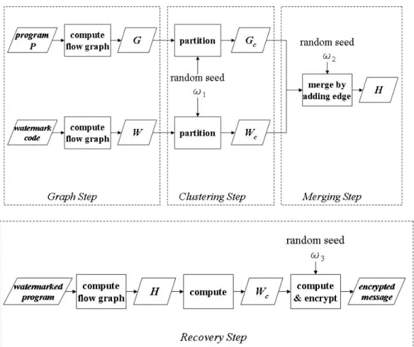
(14) Chapter 2 Related Work. In this chapter, related software watermark algorithms will be introduced. At first, a software watermark framework which can adapt different graph encodings is published by Ramarathnam Venkatesan [5]. Static and dynamic software watermark algorithms both have each related graph-based encodings. QP algorithm is a significant concept to embed the watermark through graph-based encoding. QPS algorithm use color modification to improve QP algorithm. And CT algorithm provides a runtime execution algorithm to embed or recognize watermark.. 2.1 Graph Theoretic Approach for Software Watermarking Graph Theoretic Approach which is proposed by Venkatesan, Vazirani, and Sinha [5] provides a tool for software tamper resistance and against the graph based attack. In this approach, weak connection means that a link or function call between program P and watermark W is only a single edge between two subgraphs which are parsed from P and W. To prevent being identified as weak connection, graphs are efficiently separated into subgraphs which will be merged by adding edges, and graphs will be well connected. Subgraphs of W must be locally indistinguishable from P. Based on well connection and locally indistinguishableness. The steps of graph algorithm are shown as Figure 2.1. For given program P, watermark code W, secret keys ω1, ω2 and ω3, and integer m: Graph step: Flow graph G which has basic block as nodes and control flow or function calls as edges is computed from P. Similarly for W. G and W are both digraphs. Clustering step: Using ω1 as random seed to partition G into n clusters, so that edges straddling across clusters are minimized. Let Gc be the graph where each node corresponds to a cluster in G and there is an edge between two nodes if the corresponding clusters in G have an edge going 4.

(15) across them. Wc is yielded in the same way as Gc to produces undirected graphs of small order. Merging step: Edges are added between Gc and Wc using a random process. The edges are added by a random process: when the node is v, the current values are dgg and dgw, the number of nodes adjacent to v in Gc and Wc respectively. Let Pgg = d gg (d gg + d gw ) and Pgw = d gw (d gg + d gw ) . The next random node in Gc will be visited with probability Pgw or a node in Wc with probability Pgg and secret key ω2 will make the choices. An edge is added between node v and its next random node. Repeat the step until the resultant graph H yield. Recovery step: Finally, Wc is compute and encrypted with secret key ω3.. Figure 2.1 Graph Theoretic Approach. 2.2 Static Watermark Algorithms In static watermark algorithm, watermarks are stored in the application executable itself. Static 5.

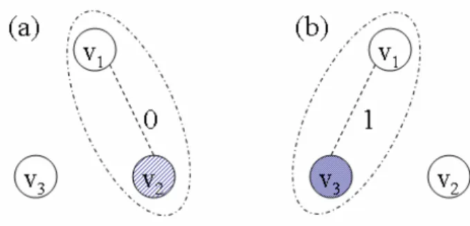
(16) watermark may exist as code or data stored in the section of the program. QP and QPS are classified into this group.. 2.2.1 QP Algorithm Qu and Potkonjak have proposed QP algorithm for embedding a watermark. QP algorithm contains three kinds of watermark algorithms and adding edges is the algorithm we choose to study and improve. In this paper, for a given graph G (V, E) and a message M to be embedded in G. Let vertices set V = (v0, v1… vn-1), edges set E and the message is encrypted into a binary string M = m0 m1… (By stream ciphers, block ciphers or cryptographic hash functions). Embedding phase: First, a vertex vi is selected from given graph G (V, E) and find the nearest two vertices vi1 and vi2 for all i < i1 < i2 (mod n) which are not connected to vi, where means (vi, vi1), (vi,. vi2) ∉ E. And the rule for embedding according to mi is as follows: If mi = 0, (νi, vi1) is put into E’, means the edge between νi and vi1 is added. If mi = 1, (νi, vi2) is put into E’, means the edge between νi and vi2 is added. After the message M = m0 m1…are entirely embedded, a new graph G’ (V, E’) which have new edges set is reported. For example, in Figure 2.2, a message M = 510 = 1012 has been embedded into a 6 vertices graph by 3 edges and each edge presents one bit of message M. The essence of this algorithm is to add an extra edge between two vertices, and these two vertices have to be colored by different colors.. Figure 2.2 An Example of QP Algorithm 6.

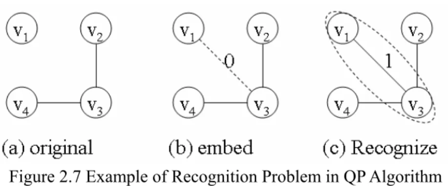
(17) Figure 2.3 QP Recognition Algorithm. Recognition phase: In given graph G’ (V, E’), each (νi, vj) is the vertices pair that one bit of the embedded message can be obtained. For each (νi, vj), j > i (mod n), the bit extraction is done by examining the number of vertices between νi and vj are not connected to νi. There will be three cases to consider: CaseⅠ: If there is no vertex which is not connected to νi, a 0 bit will be extracted. The example is shown as Figure 2.3 (a). CaseⅡ: If there is only one vertex which is not connected to νi, a 1 bit will be extracted. The example is shown as Figure 2.3 (b). CaseⅢ: If there is more than one vertex which is not connected to νi, then reverse the order of νi and vj and repeat the extraction process.. 2.2.2 QPS Algorithm Myles and Collberg pointed out the error in QP algorithm, recognition failure. They provide two example of recognition failure as follow: Example 1: Consider a graph G (V, E) as Figure 2.4 (a) and the message M = m1m2 is 00. The embedding phase is illustrated as Figure 2.3 (b). At first, νi = v0, vi1 = v2 and vi2 = v3 are selected to embed m1 = 0 by adding edge between v0 and v2. And νi = v3, vi1 = v0 and vi2 = v1 are selected to embed m2 = 0 by adding edge between v3 and v0. New graph G’ (V, E’) is obtained as Figure 2.3 (c). In recognition phase, m1 = 0 is found by examining the number of vertices not connected to v0 between v0 and v2. And m2 = 1 is found by examining the number of vertices not connected to v3 7.

(18) between v0 and v3. The inaccurate message 01 is extracted when 00 was the embedded message.. Figure 2.4 Failure Recognition of QP Algorithm. Example 2: When we embed the message 101 in the graph G (V, E) as Figure 2.5 (a), the new graph. G’ (V, E’) is obtained as Figure 2.5 (b). By following the recognition algorithm, the message 1001 is recovered.. Figure 2.5 Failure Recognition of QP Algorithm. They considered the unpredictability of coloring for the vertices as the inaccurate message recognition of QP algorithm. To eliminate the unpredictability, QPS algorithm places additional constraints on which vertices can be selected for a triple. In this paper, for a given a graph G = (V,. E), a set of three vertices {v1, v2, v3} is considered a triple if 1. v1, v2, v3 ∈ V, 2. (v1, v2), (v1, v3), (v2, v3) ∉ E And for a given a n-colorable graph G = (V, E), a set of three vertices {v1, v2, v3} is considered a 8.

(19) colored triple if. 1. v1, v2, v3 ∈ V, 2. (v1, v2), (v1, v3), (v2, v3) ∉ E, and 3. {v1, v2, v3} are all colored the same color.. Embedding phase: Select a vertex vi which is not must already in a triple. Find the nearest two vertices vi1 and vi1 which are the same color as vi and not already in a triple. An additional register allocator would be used to record related color of selected triple as (v'i, v'i1, v'i2). And the rule for embedding according to mi is as follows: If mi = 0, add edge (νi, vi1) and change the color (ν'i, v'i1). If mi = 1, add edge (νi, vi2). The key idea of QPS embedding algorithm is to select the triples so that they are isolated units that will not affect other vertices in the graph. In addition, they use a specially designed register allocator which only changes the coloring of one of the two vertices involved in the added edge and no other vertices in the graph. Recognition phase: QPS recognition algorithm works by identifying triples which had been selected in the embedding phase. A triple (vi, vi1, vi2) has been identified, and its related colored. triple, (v'i, v'i1, v'i2), is examined. If v'i and v'i1 are different color, a 0 was embedded, otherwise a 1 was embedded.. 2.2.3 Problems The colors of vertices provide starting-point to discuss. In QP embedding algorithm, an extra edge is added between two vertices and these two vertices which may not be necessary in the original graph G will be colored by different colors. In QP recognition algorithm, we will find colors between two vertices are not accurate feature to observe one bit of message had been embedded.. 9.

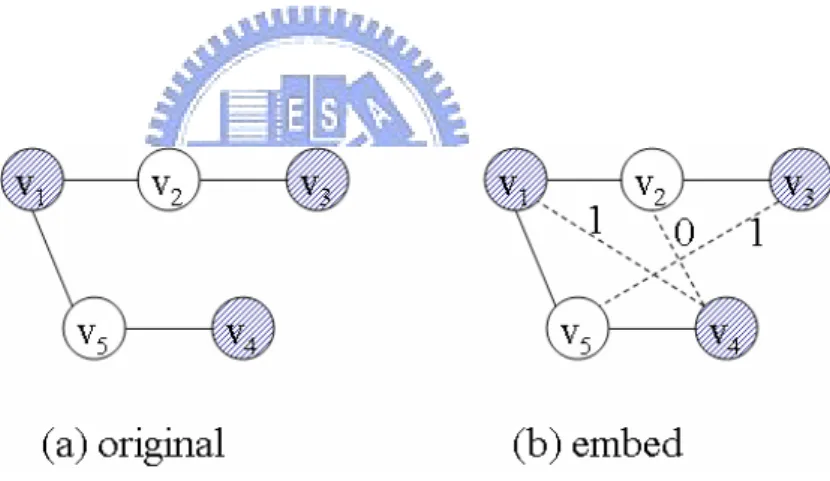
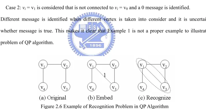
(20) The coloring feature in QP algorithm is ambiguous. This results in bad performance in embedding and recognizing watermark information. In Example 1, when νi = v3, vi1 = v0 and vi2 = v1 are selected to embed m2 = 0, QP embedding algorithm which is defined as i < i1 < i2 (mod n) has been mistaken about. Unpredictable error could occur when we embed the message and neglect the definition i < i1 < i2 (mod n). For illustration, as Figure 2.6, the message M = 1 will be embedded into original graph, as Figure 2.6 (a). In embedding phase, νi = v2, vi1 = v3 and vi2 = v0 are selected to embed M = 1 as Figure 2.6 (b). In recognition phase, the message will be identified by examining the number of vertices not connected to v0 between v0 and v2 and there are two cases can take into consider: Case 1: νi = v3 is considered that is not connected to νi = v0 and a 1 message is identified. Case 2: νi = v1 is considered that is not connected to νi = v0 and a 0 message is identified. Different message is identified when different vertex is taken into consider and it is uncertain whether message is true. This makes it clear that Example 1 is not a proper example to illustrate problem of QP algorithm.. Figure 2.6 Example of Recognition Problem in QP Algorithm Some problems occur when the definition is followed already. To illustrate, Example 3 and 4 are applied to consider and there is no need to go into details about the color between vertices:. 10.

(21) Figure 2.7 Example of Recognition Problem in QP Algorithm Example 3: Consider a graph G (V, E) as Figure 2.7 (a) and the message M = 0. The embedding phase is illustrated as Figure 2.7 (b), and νi = v0, vi1 = v2 and vi2 = v3 are selected to embed M = 0 by adding edge between v0 and v2. New graph G’ (V, E’) is obtained as Figure 2.7 (c). In recognition phase, M = 1 is found by examining the number of vertices not connected to v0 between v0 and v2. The inaccurate message 1 is extracted when 0 was the embedded message.. Figure 2.8 Example of Recognition Problem in QP Algorithm Example 4: Consider a graph G (V, E) as Figure 2.8 (a) and the message M = 1. The embedding phase is illustrated as Figure 2.8 (b), and νi = v0, vi1 = v2 and vi2 = v3 are selected to embed M = 0 by adding edge between v0 and v3. New graph G’ (V, E’) is obtained as Figure 2.8 (c). In recognition phase, the number of vertices not connected to νi = v0 between νi = v0 and νj = v3 is 2, and the same we reverse the order as νi = v3 and νj = v0. It is an undefined case that an unknown message is extracted if the number is 2.. The cause of the problem can be traced back to the assumption of embedding phase of QP algorithm: find the nearest two vertices vi1 and vi2 which are not connected to vi. We define the graph have 11.

(22) “vertices pair” which means the nearest vertices vi1 and vi2 are not connected to vi. When vi is selected, there are many vertices pairs {vi1, vi2} can be selected to embed the message. In Figure 2.6, when vi = v0, there are two vertices pairs, {v1, v2} and {v2, v3} for being selected to embed the message. Correct message will be extracted if {v1, v2} is selected. In Example 3, an inaccurate 1 message is extracted when {v2, v3} is selected. In the same way, in Figure 2.8, correct message will be extracted if {v1, v2} is selected and inaccurate message will be extracted if {v2, v3} is selected. Take a more carefully look into the selection of vertices pairs in the embedding phase and we find the result: Only if the vertices pair is the nearest to vi is restricted to selected, the message must be correct is extracted. This restrict can be treated as the definition in QP embedding phase.. 2.3 Dynamic Watermark Algorithm The basic concept of dynamic watermark algorithm is to embed watermark information to the running state of a program. In the other words, the watermark information can be embedded and extracted at runtime and thus make the disclosure more difficult. However, the implementation of dynamic watermark algorithm is difficult for most programming languages. Generally, Java-based language can implement algorithm easily. It can divide into four phases: Annotation: Adding annotation (or mark) points into the application to be watermarked before the watermark can be embedded. Functions will be inserted into these annotation points. These functions perform no action and simply indicate to the locations where watermark can be inserted. Locations are preferred mark locations that allocate objects and manipulate pointers and directly depend on user input. Hot spots and non-deterministically execution should avoid mark locations. Tracing: A tracing run of the program will be performed after the application has been annotated. Some annotation points will be selected after the tracing run. These annotation points will be the location where watermark-building code will later be inserted. Embedding: Hence, embedding of watermark will start when the application has been traced. The input will be converted into an integer. From the integer, a graph G is generated to embed. The 12.

(23) embedding of watermark is divided into four steps: 1.. Watermark W is embedded by generating graph G.. 2.. Generating an intermediate code to build this graph and translate into a Java method.. 3.. Replace the functions in annotation phase with these new functions.. 4.. New Java method file will be executed to build the graph G on the heap.. A single graph encoding method is not expected to fill requirements (high bit rate, high resilience to attack, etc.) in CT algorithm. Develop a library of graph encoding for building watermark graphs which have different characters instead. There are five kinds of graph encoding methods are implemented: Permutation encoding、Radix encoding、Parent-pointer trees、Reducible permutation graph and Planted plane cubic trees. Extraction: In watermarked application, extraction is run as a sub-process under debugging. The secret input sequences are exactly entered as input and same mark allocations will be hit during tracing run. If the last part of input has been entered, the heap is examined for graphs that could potentially be a complete watermark graphs. Number of watermark will be extracted from graphs and reported.. There are five kinds of graph encoding algorithms which are implemented in CT algorithm. Permutation, Radix and Parent-pointer tree encoding algorithm have higher date rate than other algorithm. The detail is given respectively as follow:. Figure 2.9 Example of Permutation Encoding Algorithm Permutation Encoding: A watermark integer in the range [0…n-1] can be shown by permuting the. 13.

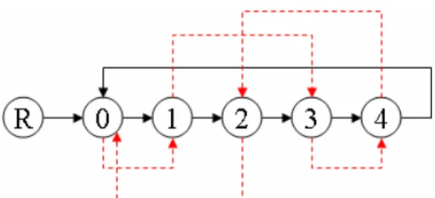
(24) numbers 0, ..., n − 1 , the mapping of permutation will represent a number. For an example, the original A =< 0, 1, 2, 3, 4, 5, 6, 7 >. and. a. watermark. is. 1000,. the. permuted. A. will. be A =< 0, 7, 2, 1, 4, 3, 6, 5 > to represent the watermark. Permutation can be constructed by a singly-linked, circular list data structure, such as Figure 2.9.. Radix Encoding: A Radix graph is a circular linked list with n lengths, order of node represent the number of exponent with base-n digit and data pointer is the coefficient. A null-pointer encodes a 0, a self-pointer is a 1, and a pointer to next node encodes a 2, and so on. Take Figure 2.10 as an example, 3 × 6 4 + 2 × 6 3 + 3 × 6 2 + 4 × 61 + 1 × 6 0 can be represented by the graph.. Figure 2.10 Example of Radix Encoding Algorithm. Parent-pointer trees encoding (PP trees): This encoding algorithm can be described as. enumerations of graphs. The idea is that the watermark number n can be represented by the index of the watermark graph in a table of enumeration and the number of nodes depends on your watermark. Figure 2.11 is an example which represents the number 1, 2, 20 and 21.. Figure 2.11 Example of PP Tree Encoding Algorithm 14.

(25) 2.4 Summary In this chapter, we introduce advantage and disadvantage of some famous framework and algorithms. Based on these characters, we will design and modify our proposed software watermark framework and algorithms.. 15.

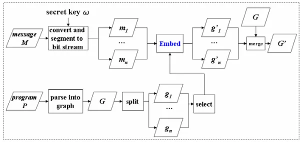
(26) Chapter 3 The Proposed Software Watermarking Framework. As described in the previous chapter, we explain the problems of failure recognition, low bit rate and color in QP and QPS algorithm. We also proposed static software watermark algorithms by leveraging the concepts in CT dynamic algorithm. The proposed static watermark algorithms will make the improvement on these characters: Easier in constructing and extracting Higher bit rates Better robust from common attacks More programming languages. We proposed a flexible framework to adopt not only proposed graph encoding algorithms but also other graph algorithms. To construct and extract watermark easily, we modify the heavy procedure of random walk in Graph Theoretic Approach. It is also implemented easily with more kinds of programming languages.. 3.1 Framework Framework can be divided into two phases: embedding and recognition phases. Embedding and recognition phase are shown with Figure 3.1 and Figure 3.3 separately. In embedding phase, process proceeds through three steps: Transformation step: Program P is parsed into graph G which is constructed by vertices and edges.. Each vertex of graph represents a basic block consisting of instructions. Each edge will be a directed edge represents a function call between two basic blocks. Order of vertices is arranged by depth-first search (DFS) algorithm. Message M can be a statement or special integer in binary 16.

(27) format. To make binary conversion, the hash function or other transform function can also be adopted to achieve higher security. To increase the complexity and improve the privacy, graph G is segmented into n subgraphs, {g1 , g 2 ,L, g n }, where gi is one of the subgraph of G. The representation of the gi shown as G = {g i 1 ≤ i ≤ n}, where n is the number of subgraphs. Message M is also segmented into n fragmental messages, {m1 , m2 ,L, mn }, using the random seed ω, where mi is one of the fragmental messages of M. The representation of the mi shown as M = {mi 1 ≤ i ≤ n}, where n is the number of subgraphs. Each subgraph is constructed according to the vertices selecting rule that make each subgraph which is decided by the corresponding fragmental message being embedded successfully.. Figure 3.1 Embedding Phase of Proposed Framework. The vertices selecting rule is defined as follow: 1. Select the vertex in the higher level of sub-graph as the first-selected vertex. 2. Select the vertices which aren’t the children of first vertex of sub-graph.. Each subgraph should have these characters:. 17.

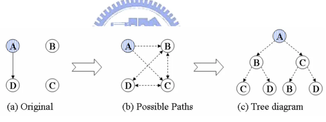
(28) 1. The size of subgraph is decided by corresponding fragmental message 2. A sub-graph should contain at least three vertices. 3. If sub-graph is constructed from k vertices, fragmental message should be k-2 bits.. Embed step: When fragmental messages and subgraphs are generated, the next move is selecting. the algorithm of graph encoding. There are three kinds of graph encoding algorithms: link encoding (LE)、color encoding (CE) and link color encoding (LCE). If LE or LCE is selected, path analysis will proceed. During the process of path analysis, as Figure 3.2, subgraph and the path which has more levels for embedding is analyzed by tree diagram. First vertex is selected according to the result from path analysis. Follow on the first vertex, fragmental message is embedded into its corresponding subgraph by adding directed edge between two vertices.. Figure 3.2 Example of Path Analysis. Merge step: The last step is merging original graph G and each subgraph into new graph. Directed. edge is added between two vertices in original graph if the same vertices in subgraph have been embedded a bit of fragmental message. Color of vertices in original graph will be tampered according to the same vertices in subgraph. Finally, a new graph G’ contains the embedded message is generated.. 18.

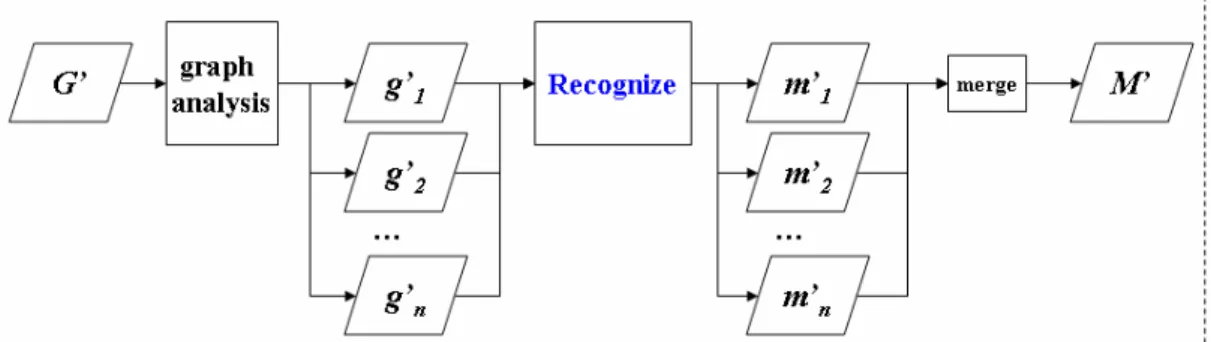
(29) Figure 3.3 Recognition Phase of Proposed Framework. In recognition phase, there are two steps: Recognition step: When watermarked graph G’ is received, information of subgraphs, vertices and. its corresponding color, and edges are also known. Algorithm of graph encoding which was used to embed the message is also analyzed and found. In the light of information, graph G’ is segmented into n subgraphs {g1′ , g 2′ , L, g ′n } , where g’i is one of the subgraph of watermarked graph G’. The representation of the gi is shown as G ' = {g ' i 1 ≤ i ≤ n} , where n is the number of subgraphs. According. to. that. {m'1 , m' 2 ,L, m' n } are. graph. encoding. recognition. algorithm,. the. fragmental. messages. extracted from each subgraph, where m’i is one of message M’. The. representation of the mi is shown as M ' = {m' i 1 ≤ i ≤ n}, where n is the number of subgraphs. Message processing step: Combine each fragmental message into new message m’. It is not. necessary that new message M’ must be equal to original message M’ if we can verify the correct hidden information from M’.. Figure 3.4 is an example of proposed framework in embedding phase: 1. Input is m = 1011 and program P. 2. P is parsed into graph G, and index is arranged by DFS algorithm. 3. MB is segmented into two fragmental messages m1 = 10 and m2 = 11. G is also segmented into two subgraphs g1 and g2 with vertices selecting rule.. 19.

(30) 4. When link encoding algorithm is selected, each subgraph is analyzed by path analysis and the pivot vertex is decided. Then, fragmental messages bi1 and bi2 are embedded into subgraphs g1 and g2. 5. Merge graph G and subgraphs g1 and g2 into new graph G’.. Figure 3.4 Example of Proposed Embedding Phase Framework. 3.2 Proposed Graph Encoding Algorithms In this section, we will introduce proposed graph encoding algorithms. At first, the definition is as follows: Given fragmental message mi ,represent as {bi1 , bi 2 , L, bi n } , where mi = {bij 1 ≤ j ≤ β }, β is number of bit in fragmental message and a subgraph Gi (Vi, Ei) which contains vertices set Vi and edges set Ei. Vertices pair, {va1, va2} contains nearest two vertices va1 and va2, and is also the nearest vertices. pair not connected to va. Edges (va, va1), (va, va2) are not in edges set Ei.. 3.2.1 Link Encoding (LE). This algorithm can have improvement in robust by the way of link list. Pivot vertex is the vertex which is selected according to path analysis [24] [22] and subgraph will have the higher capacity 20.

(31) for embedding message.. Figure 3.5 Example of Link Encoding in Embedding Phase. Input: watermark m=b1b2…bn and a graph G(V,E) Output: G’(V, E’), pivot vertex vp, remaining vertex vr Pseudo Code: vp = path_analyze(gi,n); if vp is not found return NULL; va = vp; V’ = V; foreach bit bj { search V’ and find the vertices pair (va1,va2) that are nearest but not connected to V’= V’- {va}; if bj=0 E’ = E ∪(va,va1); va = va1; else E’ = E ∪(va,va2); va = va2; } vr = the last element in V’; return G’(V, E’);. va. Figure 3.6 Pseudo Code of LE Embedding Algorithm. Embedding phase: va is selected pivot vertex. For the first message bi1, vertices pair {va1, va2} is. the nearest vertices pair not connected to va is found. If bi1 = 0, directed edge (Va, Va1) is added. Else, bi1 = 1, directed edge (va, va2) is added. Then, the vertex va is treated as invisible vertex and its. connected vertex (va1 or va2) is treated as new pivot vertex which will be embedded with the next message m1. Repeat the step until mi = bi1 bi2…bin are all embedded into subgraph Gi (Vi, Ei) and. 21.

(32) new graph G’i (V’i, E’i) will be generated. We will find that the last one vertex which is not used during the embedding step and the information of pivot vertex and remaining vertex is useful for robust. Figure 3.5 is an example of link encoding in embedding phase. For given subgraph, as Figure 3.5 (a), mi = 0011 and pivot vertex v1 is selected. First directed edge (v1, v2) is added according to bi1 = 0 and {v2, v3} is the nearest vertices pair not connected to v1. v2 is treated as new pivot vertex and v1 is treated as invisible vertex when bi2 = 0 is ready for embedding. Repeat the. step as Figure 3.5 (b) until mi = bi1 bi2 bi3 bi4 are embedded. The pseudo code for the embedding phase in LE algorithm is described in Figure 3.6.. Input: watermarked graph G’(V’,E’), pivot vertex vp, remaining vertex Output: watermark m=b1b2…bn Algorithm: V’= V; va = vp; V’= V’- {va}; foreach j between 1 and n { foreach vertex vk in V’ if vk is adjacent to va count = 0; foreach q between k and a if vq is not connected to va count ++; if count == 0 bj=0; va = vk; elseif count == 1 bj=1; va = vk; else continue; //check next adjacent vertex of va V’= V’- {va}; } vr’ = the last element in V’; if vr’ == vr return m; else return NULL;. vr. Figure 3.7 Pseudo Code of LE Recognition Algorithm. Recognition phase: How can we extract the message from graph? Given the graph G’i (V’i, E’i) and. the information of pivot vertex va, find the number of vertices not connected to va between va and its connected vertex. If the number is zero, bi1 is 0, and if the number is 1, bi1 is 1. For the vertex 22.

(33) connected to va and treating va as an invisible vertex, the next message will be extracted. Repeat the step until that there is only one vertex in subgraph and compare this vertex with remaining vertex. We will make sure the message is correct if the answer is “the same”. The pseudo code for the recognition phase in LE algorithm is described in Figure 3.7.. 3.2.2 Color Encoding (CE). The function of color is applied for increasing bit rate in color encoding algorithm. All the vertices in subgraph are the same color in original. The color rule is defined as follows: va and its connected vertex vb are same color, a 00 message is embedded. va and its connected vertex vb are different color, a 01 message is embedded.. Input: watermark m=b1b2…bn, a graph G(V,E) Output: G’ (V, E’), vertex color set C = {c1,c2,…cn} and an embedding vertex set Vx. Algorithm: C = initialize_vertex_colors(V); V’ = V; Vx = φ ; foreach bjbj+1 { va = smallest(V’); va1, va2 = closest_vertices_pair(va); switch (bjbj+1) { case 00: E’ = E’ ∪ (va, va2); break; case 01: E’ = E’ ∪ (va, va2); ca2 = new color different than ca2 //change va2’s color; break; case 11: E’ = E’ ∪ (va, va1); break; case 10 : E’ = E’ ∪ (va, va1); ca1 = new color different than ca1 //change va1’s color; break; } V’ = V’ – {va}; Vx = Vx + {va}; } return G’(V,E’), C’;. Figure 3.8 Pseudo Code of CE Embedding Algorithm. Embedding phase: For mi = bi1 bi2…bin, each fragment message is a 2-bit message in this method. 23.

(34) Find vertices pair {va1, va2} that are nearest pair and not connected to va. bij bi(j+1) = 00. (va, va2) is added, va and va2 are same color.. bij bi(j+1) = 01. (va, va2) is added, va and va2 are different color.. bij bi(j+1) = 11 (va, va1) is added, va and va1 are same color. bij bi(j+1) = 10. (va, va1) is added, va and va1 are different color.. The new graph G’i (V’i, E’i) which contains new edges set E’i and new vertices set V’i with its related information of color is generated. The pseudo code for the embedding phase in CE algorithm is described in Figure 3.8. Figure 3.9 is a simple example of color encoding in embedding phase. At first, mi = 1101 is segmented into 11 and 01. v1 is selected as va, and {v2, v3} is the nearest vertices pair that are not connected to v1. For the first two bits 11, the directed edge (v1, v2) is added and v1 and v2 are still same color. And the next message, v2 is selected as va, and {v3, v4} is the nearest vertices pair that are not connected to v2. For the next two bits 01, the directed edge (v2, v4) is added and v2 and v4 are colored by different color.. Figure 3.9 Example of Color Encoding in Embedding Phase. Recognition phase: Given the graph G’i (V’i, E’i) and vertices set with information of color. Find. the number of vertices not connected to va between va and its connected vertex vb. The embedded bit. 24.

(35) is extracted according the rule as follows: The number is 0, va and vb are same color, then mi = 11 The number is 0, va and vb are different color, then mi = 10 The number is 1, va and vb are same color, then mi = 00 The number is 1, va and vb are different color, then mi = 01 The pseudo code for the recognition phase in CE algorithm is described in Figure 3.10.. Input: a graph G(V,E), an embedding vertex set Vx and its color set C Output: m=b1b2…bn Algorithm: do { va = first element in Vx; Vx = Vx – {va}; find the closest vertices va1, va2 that are not connected to va; count for the vertices whose indices are in between va1 and va2, and are not connected to switch (count) { case 0: if (va, va1) exists in E and ca == ca1 bjbj+1=11; elseif (va, va1) exists in E and ca != ca1 bjbj+1=10; elseif (va, va2) exists in E and ca == ca2 bjbj+1=11; elseif (va, va2) exists in E and ca != ca2 bjbj+1=10; break; case 1: if (va, va1) exists in E and ca == ca1 bjbj+1=00; elseif (va, va1) exists in E and ca != ca1 bjbj+1=01; elseif (va, va2) exists in E and ca == ca2 bjbj+1=00; elseif (va, va2) exists in E and ca != ca2 bjbj+1=01; break; } } while (Vx) return m;. va;. Figure 3.10: Pseudo Code of CE Recognition Algorithm. 3.2.3 Link with Color Encoding (LCE). The third method is link with color encoding, as implied in the name, and is combined with link encoding and color encoding. LCE method is successful to have the higher robust and bit rate. 25.

(36) Follow the definition of link encoding and color encoding, this method is introduced as follow: Embedding phase: Given message mi = bi1 bi2…bin and a subgraph Gi (Vi, Ei), va is selected pivot. vertex. Find vertices pair {va1, va2} is the nearest vertices pair not connected to va. First two bit of. message bi1 bi2 are embedded according to the rule as follows: bi1 bi2 = 00 (va, va2) is added, va and va2 are same color. bi1 bi2 = 01 (va, va2) is added, va and va2 are different color. bi1 bi2 = 11 (va, va1) is added, va and va1 are same color. bi1 bi2 = 10 (va, va1) is added, va and va1 are different color.. Then, the pivot vertex va is treated as invisible vertex and its connected vertex is treated as new pivot vertex which will be embedded with the next two bits bi3 bi4. Repeat the step until mi = bi1 bi2…bin are all embedded into subgraph Gi (Vi, Ei) and new graph G’i (V’i, E’i) will be generated.. The pseudo code for the embedding phase in LCE algorithm is described in Figure 3.11. Figure 3.12 is an example with LCE method in embedding phase.. Input: G(V,E), m=b1b2…bn, and color set C = {c1,c2,…cn} Output: G’(V,E’), C’, the pivot vertex vp, the remaining vertex vr Algorithm: foreach bjbj+1 { select a pivot vertex vp from V; let va = vp; start from the vertex va, where a is the smallest vertex index in V; find the closest vertices va1, va2 that are not connected to va; switch (bjbj+1) { case 00: add edge (va, va2) to E; va = va2 ; break; case 01: add edge (va, va2) to E; ca2 = different color from ca; va = va2 ; break; Case 11: add edge (va, va1) to E; va = va1 ; break; Case 10: add edge (va, va1) to E; ca1 = different color from ca; va = va1 ; break;. 26.

(37) } } return G’(V,E’) and C’;. Figure 3.11: Pseudo Code of LCE Embedding Algorithm. Figure 3.12: Example of Link with Color Encoding in Embedding Phase. Recognition phase: Given the graph G’i (V’i, E’i) and vertices set with information of color. Find. the number of vertices not connected to va between va and its connected vertex vb. The first embedded bits bi1 bi2 are extracted according the rule as follows: The number is 0, va and vb are same color, then bi1 bi2 = 11 The number is 0, va and vb are different color, then bi1 bi2 = 10 The number is 1, va and vb are same color, then bi1 bi2 = 00 The number is 1, va and vb are different color, then bi1 bi2 = 01 With the vertex vb connected to va and treating va as an invisible vertex, the next message m1 will be extracted. Repeat the step until that there is only one vertex in subgraph and compare this vertex with remaining vertex. We will make sure the message is correct if answer is “the same”. The pseudo code for the recognition phase in LCE algorithm is described in Figure 3.13.. Input: a watermarked graph G’(V,E’), the pivot vertex vp, the remaining vertex Output: m=b1b2…bn Algorithm: start from the pivot vertex vp; let visiting vertex va equals to vp; find the closest vertices va1, va2 that are not connected to va; foreach two bits bjbj+1. 27. vr. and the color set C.

(38) { count for the vertices whose indices switch (count) { case 0: if (va, va1) exists in E and bjbj+1=11; elseif (va, va1) exists in E bjbj+1=10; elseif (va, va2) exists in E bjbj+1=11; elseif (va, va2) exists in E bjbj+1=10; break; case 1: if (va, va1) exists in E and bjbj+1=00; elseif (va, va1) exists in E bjbj+1=01; elseif (va, va2) exists in E bjbj+1=00; elseif (va, va2) exists in E bjbj+1=01; break; }. are in between a1 and a2, and are not connected to. va;. ca == ca1 and ca != ca1 and ca == ca2 and ca != ca2. ca == ca1 and ca != ca1 and ca == ca2 and ca != ca2. } return mi;. Figure 3.13: Pseudo Code of LCE Recognition Algorithm. 3.3 Example In this section, we present how the proposed graph encoding algorithms can be applied to a example program shown in Figure 3.14, a prime number generator that generates prime numbers no larger than integer a. A two-bit message 01 will be embedded into the program. int k(int); int main() { int a, b, sum; printf("insert a prime number \n"); scanf("%d",&a); for(sum=0,b=2;b<=a;b++) { if(k(b)) printf("%3d",b); sum+=b; } return 0; } int k(int b) { int i; for(i=2;i<=b/2;i++) if(b%i==0) return 0; return 1; }. //v1 //v2 //v3 //v4 //v5 //v6. Figure 3.14: Example Program In the phase of transform, we select the blocks as vertices and the program is parsed into graph as 28.

(39) Figure 3.15. With the length of message, a four-vertex graph is prerequisite. We select a four-vertex graph including vertices set V = {v1, v3, v5, v6} and edges set E = {(v5, v6)}. According the analysis of path, v1 is selected as pivot vertex. In the embedding phase, LE algorithm is used to embed the message 01 by adding the edges (v1, v3) and (v3, v6) as Figure 3. The watermarked program and its related parsed graph is shown as Figure 4 and Figure 5 respectively.. Figure 3.15: The Parsed Program. Figure 3.16: The Graph of Embedding int k(int); int main() { int s, t; int a, b, sum; if ((s^2+s)%2) goto s2 printf("insert a prime number \n"); v3: scanf("%d",&a); if (!((t^2+t+1)%2)) goto v5 for(sum=0,b=2;b<=a;b++) { if(k(b)) v5: printf("%3d",b); sum+=b; } return 0; }. //v1 //v2 //v3 //v4 //v5 //v6. 29.

(40) Figure 3.17: The Watermarked Program. Figure 3.18: The Parsed Watermarked Program. 3.4 Path Analysis Path analysis is a useful tool which is not only finding the longer path buy also providing a test and verify. Take Figure 3.19 as an example, we introduce the concept of path analysis. Original graph is given, as Figure 3.19 (a) is a 4-vertices diagram and v1 is selected as pivot vertex. LE algorithm is used to embed a 2-bit message with 4-vertices diagram. For a 2-bit message, Figure 3.19 (b) shows 4 possible paths to embed 4 possible messages. Given another graph as Figure 3.20 (a), it is obvious to find that embedding process encounters problem if the message is 00 or 01. And graph as Figure 3.21 (a) can’t be embedded into any message if pivot vertex is v1.. Figure 3.19 Example of 4 Possible Paths with 4 Vertices and LE Algorithm. 30.

(41) Figure 3.20 Example of 2 Possible Paths with 4 Vertices and LE Algorithm. Figure 3.21 Example of Zero Possible Paths with 4 Vertices and LE Algorithm. The situation of success and failure embedding can be checked with path analysis. In the same way, possible paths are analyzed and found if a vertex is selected as pivot vertex. Take Figure 3.19 as an example, the graph diagram is as Figure 3.22 (a). The graph diagram shows the possible paths from the pivot vertex. From v1, the vertices pair (v2, v3) is the nearest one not connected to v1 and (v1, v4) will not be a possible path. The graph diagram will expand upon a tree diagram as Fig 3.22 (b) under the rule of LE encoding algorithm. In tree diagram, it is obvious to find four possible paths which are corresponding to Figure 3.19 (b).. Figure 3.22 Example of Path Analysis with 4 Vertices and LE Algorithm. Figure 3.23 is another example corresponding to Figure 3.20. The graph diagram shows the possible 31.

(42) paths from the pivot vertex, v1. The tree diagram as Fig 3.23 (b) will expand from graph diagram. There are only two possible paths under the rule of LE encoding algorithm.. Figure 3.23 Example of Path Analysis with 2 Vertices and LE Algorithm. 3.5 Error Detection Path analysis described in the previous section can also be applied in error detection. According to the information of pivot vertex and remaining vertex, we can verify that some bits of message are in error or not. Figure 3.24 shows an example of error detection:. Figure 3.24 Example of Error Detection. Given watermarked graph G′ with LE algorithm as Figure 3.24 (a), start and remaining vertex are v1 and v4 respectively. From the pivot vertex v1, to fit in with the information of remaining v4, an 32.

(43) embedding path E = {(v1 , v 2 ), (v 2 , v3 ), (v3 , v5 ), (v5 , v6 )} is found. A Hamiltonian path can be found if we add a virtual directed path (v6, v4). The message is extracted correctly by LE recognition algorithm. Figure 3.24 (b) shows that an error occurs in edge (v2, v3) and an altered edge (v2, v6) instead. From the pivot vertex v1, with the information of remaining v4, we can’t find any possible path. Critical error occurs in graph if there is Hamiltonian path is found and we can use path analysis to recover the message. At first, from LE embedding algorithm, we analyze the graph and find that edge (v1, v2) should be correct message. The next pivot vertex is v2 and {v3, v4} is the nearest vertices pair and there should be an edge (v2, v3) or (v2, v4). According to the information of the edge (v3, v5), we can recover the edge (v2, v3) and find the correct embedding path. A Hamiltonian path is found if we add a virtual directed path (v5, v4). The message are recovered and extracted correctly by LE recognition algorithm.. 3.6 Summary In this chapter, we propose a graph-based watermark framework can adopt more than three kinds of graph encoding algorithms. According to the requirement of robust and bit rate, LE, CE and LCE algorithm can be applied respectively.. 33.

(44) Chapter 4 Analysis. After illustrating the proposed framework and algorithms, analysis and comparison with other framework and algorithms is an essential work. The performance in stealth, robust and flexibility are the criteria for software watermark algorithms.. 4.1 Security Analysis After the watermarked graph is produced, there are many kinds of adversaries. A robust watermark algorithm can prevent specific attack from extracting or destroying the embedded message. We focus on preventing the additive/subtractive attacks since the graph is constructed by vertices and edges. Thus, a graph-based watermark is vulnerable to attacks on the edges and vertices in the graph. In this section, we illustrate the software watermark attacks on graph edges and vertices. Edges additive/subtractive attack. The path analysis described in the previous section can be used to detect if there is any redundant or missing edges, which can result in destroying the watermarked information in the software module. Before the process of extraction, embedding path must be found to construct a Hamiltonian path. Single edge has been altered will be recovered as we described in last section. If few bits have been altered, we have to compare with the information of path analysis from original graph according to start and remaining vertex and graph encoding algorithm. Possible paths will be found to recover the message during comparison. Vertices additive/subtractive attack. The number of vertices is restricted by the number of bit of the message. For an example, N vertices must be matched with N+2 bit message for LE algorithm. Redundant or lost vertices will be detected by the character of graph encoding algorithm. To recover the message, we 34.

(45) have to compare with the information of path analysis from original graph according to start and remaining vertex and graph encoding algorithm. During comparison, we will find the variation of vertices and reconstruct the graph to extract the correct message. Figure 4.1 is an example of vertex subtractive attack. Adversaries have deleted the v6, and the edges (v3, v6) and (v5, v6) become null pointers. It is obviously that a vertex had been deleted or lost. The correct message can still be extracted by rebuilding the graph.. Figure 4.1 Example of Vertex Subtractive Attack. Figure 4.2 Example of Edge-flip Attack Edge-flip Attack. An edge-flip attack against the watermark reorders the edge between vertices. The outgoing of edge will be redirected to other vertices in the graph. Figure 4.2 (a) is an example of the model of attack. Adversaries try to break watermark by changing the edge (v2, v3) to be the edge (v2, v6). The malicious attack can be detected by path analysis. According the LE algorithm, the 35.

(46) original graph can be recovered. The message of watermark is still extractable correctly.. Vertex-Split Attack. The model of vertex-split attack splits the nodes in the graph. Each node will be divided into two vertices. New edges are connected between the divided vertices. With the information, the number of extracted message should be equal to embedded message in each graph or subgraph. The redundant bits of message will be found by path analysis. We can extract the broken message with some redundant 0 bits. However, we can’t recovery the correct value efficiently without the information of original graph.. 4.2 Bit rate Analysis Bit rate is an important character to estimate the performance of stealth of watermark algorithm. The definition which is given mostly is the ratio of code size of watermark to watermarked program. However, we can find that bit rate is affected by factor such as programming language, syntax of programming language…etc. Different kinds of algorithms which are used to construct the encoded graph will make bit rate have different result in comparison with other graph encoding algorithm. We want to focus on constructing the encoded graph and neglect the difference in implement, the definition is given below: The ratio of number of bits encoded by adding edges to the total size of watermarked graph. With the definition of bit rate, we will analyze each graph encoding algorithm respectively. Given a watermark MB contains n bits and graph is constructed by nodes and edges. The number of byte of graph, B = S n × N n + S e × N e , where Nn and Ne are number of node and edge respectively, Sn and Se are size of node and edge respectively. The number of byte of watermarked graph is B ′ = S n × N n + S e × N e′ and N′e is the number of edge after watermark being embedded. According to definition, bit rate is defined as (B ′ − B ) B ′ . Adding Edge Encoding (QP Algorithm) and Color Encoding: 36.

(47) It is not easy to calculate the correct value, estimation the bit rate of the common case instead. When the number of node Nn = N, the increasing number of edge is estimated as N e′ − N e = N − 1 . Based on the assumption that there will be no existed edge before embedding phase, bit rate is (B ′ − B ) B ′ = ( N − 1)S e ( NS n + ( N − 1)S e ) . Link Encoding and LC Encoding:. When the number of node Nn = N, the increasing number of edge is N e′ − N e = N − 2 . Bit rate will be (B ′ − B ) B ′ = ( N − 2)S e ( NS n + ( N − 2)S e ) based on the assumption that there is no existed edge before embedding phase. Permutation Encoding and Radix Encoding:. When the number of node contains the node of root is N n = N + 1 , the number of edge is N e = 2 N + 1 and the increased number of edge is N e′ − N e = N . Bit rate is (B ′ − B ) B ′ = NS e. ((N + 1)S n + (2 N + 1)S e ). Parent-pointer Tree Encoding:. It is also not easy to calculate the correct value of bit rate. When the number of node Nn = N, the increasing. number. of. edge. is. estimated. as. N e′ − N e = N − 1. and. bit. rate. is (B ′ − B ) B ′ = ( N − 1)S e ( NS n + ( N − 1)S e ) .. 4.3 Summary We analyze the characteristics of our graph encoding algorithms. The performance in error detection and robust is better than QP and QPS algorithm. The bit rate of each graph encoding algorithm is described in section 4.3. We will give a further discussion in next chapter.. 37.

(48) Chapter 5 Comparison. 5.1 Framework Characteristic We adapt and modify the Graph Theoretic Approach which is illustrated in section 2.1. The differences between these two frameworks are the secret key and random walk in merging step. There are three secret key for partition the graph in clustering step, choose the next node in merging step and encrypt the extracted value in recovery step respectively. In our proposed framework, we use only one secret key to segment the message into fragmental message and hence the segment of subgraph will be decided. The second difference is the random walk for merging watermark and graph. We embed each ordered fragmental message into each ordered subgraph respectively instead of using random seed to decide the next node.. Random seed Graph Theoretic. Graph/message Fragmental message vertices select segment generating. well connected graph. 3. yes. random. random. yes. 1. yes. random / user. rule. yes. Approach Proposed Framework. Table 1 : Framework Characteristic. 5.2 Bit rate of Software Watermark Algorithms As we discuss in section 4.3, bit rate of each graph encoding is analyzed, and furthermore, we will give. an. example. for. illustrating. the. comparison.. Given. an. integer. as. watermark. W = 1000010 = 10011100010000 2 and W = 14 . Let S n = kS e , bit rate is show as following: QP Algorithm/QPS Algorithm:. 38.

(49) (B ′ − B ). B ′ = ( N − 1)S e ( NS n + ( N − 1)S e ) = ( N − 1) ((k + 1)N − 1) . Let N=15 from the bit number is. 14 after estimation, and (B ′ − B ) B ′ = 14 (15k + 14 ) . Link Encoding:. (B ′ − B ). B ′ = ( N − 2)S e (NS n + ( N − 2)S e ) = ( N − 2 ) (N (k + 1) − 2) . If the bit number is 14, N=16 is. found, and (B ′ − B ) B ′ = 14 (16k + 14 ) . Color Encoding:. (B ′ − B ). B ′ = ( N − 1)S e ( NS n + ( N − 1)S e ) = ( N − 1) ((k + 1)N − 1) . Let N=8 from the bit number is. 14 after estimation, and (B ′ − B ) B ′ = 7 (8k + 7 ) Link with Encoding:. (B ′ − B ). B ′ = ( N − 2)S e (NS n + ( N − 2)S e ) = ( N − 2 ) (N (k + 1) − 2) . If the bit number is 14, N=9 is. found, and (B ′ − B ) B ′ = 7 (9k + 7 ) . Permutation Encoding:. (B ′ − B ). B ′ = NS e. ((N + 1)S n + (2 N + 1)S e ) = N ((N + 1)k + (2 N + 1)) .. N = 8 is found if the bit. number is 14, and (B ′ − B ) B ′ = 8 (9k + 17 ) . Radix Encoding:. (B ′ − B ). B ′ = NS e. ((N + 1)S n + (2 N + 1)S e ) = N ((N + 1)k + (2 N + 1)) .. N = 7 is found if the bit. number is 14, and (B ′ − B ) B ′ = 7 (8k + 15) . Parent-pointer Tree Encoding:. (B ′ − B ). B ′ = (N − 1)S e ( NS n + ( N − 1)S e ) = ( N − 1) ( Nk + ( N − 1)) Let N=8 from the bit number is. 14 after estimation, and (B ′ − B ) B ′ = 15 (16k + 15) .. According the definition, we know that ability of resilience is in inverse proportion to bit rate. In Table 2, by applying different k, we will find that the difference between each algorithm in bit rate isn’t affected. In the same situation, Radix encoding and Permutation encoding algorithms have the better performance in bit rate than LE and LCE algorithm, and QP/QPS and PP tree algorithms have worse performance in bit rate. From the information in table, we can find that “list-based” 39.

(50) algorithms have better performance than “graph-based” algorithms.. k=2. k=3. k=4. Radix. 0.225. 0.180. 0.149. Permutation. 0.228. 0.182. 0.151. PP trees. 0.319. 0.238. 0.190. QP / QPS. 0.318. 0.238. 0.189. Link Encoding. 0.304. 0.225. 0.179. Color Encoding. 0.304. 0.225. 0.179. LCE. 0.280. 0.205. 0.163. Table 2: Bit rate of Graph Encoding Algorithm. 5.3 Characteristic of Software Watermark Algorithms stealth. Flexible path selecting. Error Detection. Radix. Good. No. No. Permutation. Good. No. Yes. PP trees. Bad. No. No. QP. Bad. No. Yes. QPS. Bad. No. No. Link Encoding. Fair. Yes. Yes. Color Encoding. Fair. Yes. No. LCE. Fair. Yes. Yes. Table 3: Comparison of Graph Encoding Algorithm. 40.

(51) We compare each graph encoding algorithm with bit rate, flexible path selecting and the ability of single error detection. It is obvious that Radix have higher bit rate but with worst performance in robust and flexibility. LCE and LE will be ideal algorithm if we want have requirement of stealth, flexibility and robust.. 5.4 Summary In this chapter, we analyze the difference between proposed and related framework. The detail characteristic of each algorithm is also describes in Table 5.3.. 41.

(52) Chapter 6 Conclusion In this paper, we modify and build a flexible software watermarking framework which can adopt graph theoretical encoding algorithms. In this framework, watermark and program will be parsed into graph and merged with graph-based encoding algorithms. The hidden message with graph encodings is harder to be detected and attacked by adversaries. Program with different graph encoded watermark will have different performance in resilience and robust. QP and QPS algorithms have neither credibility nor resilience and robust. Although CT algorithm have high robust, embedding and recognition in execution time is hard and time-consuming to be constructed with non-Java language. Based on these algorithms, we design and modify three kinds of algorithms can improve resilience and robust respectively by link-type structure and application of color. Besides, proposed path analysis is an important analysis for selecting the longest embedding path and searching and analyzing the correct path. With path analysis, the watermark can be easier to be constructed and extracted, and the information of start and rest vertices can output instead of the whole information of original graph. Decrement of storage will improve the convenience and practicability for mobile code system.. 42.

(53) Chapter 7 Future Work We believe that proposed framework and graph encoding algorithms have improvement in stealth and robust. The framework can adopt not only our proposed but also other kinds of graph encoding algorithms, such as QP and QPS. Three kinds of graph encoding algorithms still have another kind of method to modify the integer of watermark into a shorter message in bit stream. If the message is shorter, the performance of stealth and resilience can be better. Encoding algorithm will be improved with robust is carried into effect. Implement is also an important work that we should achieve for verify the characteristics of each algorithm and make more improvements.. 43.

(54) Reference [1] Robert L. Davidson. and Nathan Myhrvold. “Method and system for generating and auditing a signature for a computer program,” US Patent 5,559,884, September 1996. Assignee: Microsoft Corporation. [2] Gang Qu and Miodrag Potkonjak. “Hiding Signatures in Graph Coloring Solutions,” In CA90095. USA. 1999. [3] Ginger Myles. and Christian Collberg. “Software Watermarking Through Register Allocation: Implementation, Analysis, and Attack,” ICISC 2003, LNCS 2971, pp. 274–293, 2004. [4] C. Collberg and C. Thomborson. “Software watermarking: Models and dynamic embeddings,” In POPL’99, Jan. 1999.. [5] Ramarathnam Venkatesan. Vijay Vazirani. Saurabh Sinha. “A Graph Theoretic Approach to Software Watermarking,” In 4th International Information Hiding Workshop, Pittsbutgh, PA, April 2001. [6] Lin Yuan, Gang Qu, Ankur Srivastava. “VLSI CAD tool protection by birthmarking design solutions,” In Great Lakes Symposium on VLSI, Proceedings of the 15th ACM Great Lakes symposium on VLSI table of contents, Chicago, Illinois, USA, Pages: 341 - 344, 2005. [7] Christian Collberg, Edward Carter, Stephen Kobourov, and Clark Thomborson. Error-correcting graphs. Workshop on Graphs in Computer Science (WG’2003), June 2003. [8] Christian Collberg, Clark Thomborson, and Douglas Low. Manufacturing cheap, resilient, and stralthy opaque construct. In Principles of Programming Languages 1998, [9] Fabien A.P. Peticolas, Ross J. Anderson, and Markus G. Kuhn. Attacks on copyright marking systems. In Second Workshop On Information Hinding, Portland, Oregen, April 1998. [10] Tapas Sahoo and Christian Collberg. Software Watermark in the frequency domain: Implementation. Analysis, and attacks. Technical Report TR04-07, Department of Computer Science, University of Arizona, March 2004. 44.