潛在類別迴歸模型之適合度檢定

全文

(1)國立交通大學統計學研究所碩士論文. 潛在類別迴歸模型之適合度檢定 Goodness-of-fit Test for Latent Class Regression Model. 研究生：高徽宜指導教授：黃冠華博士. 中華民國九十四年六月.

(2) 潛在類別迴歸模型之適合度檢定 Goodness-of-fit Test for Latent Class Regression Model. 研究生：高徽宜. Student：Hui-Yi Kao. 指導教授：黃冠華博士. Advisor：Dr. Guan-Hua Huang. 國立交通大學理學院統計研究所碩士論文. A thesis Submitted to Institute of Statistics College of Science National Chiao Tung University In partial Fulfillment of the Requirements For the Degree of Master in Statistics June 2005 Hsinchu Taiwan Republic of China. 中華民國九十四年六月.

(3) 潛在類別迴歸模型之適合度檢定. 研究生：高徽宜. 指導教授：黃冠華博士. 國立交通大學統計學研究所. 摘要生物醫學以及社會心理方面的研究近來越來越常使用潛在類別迴歸(latent class regression)模型來分析多重類別資料與有興趣的共變數之間的關係。在潛在類別迴歸模型中多重類別資料會被整合摘要，而與風險因子之間的關係也會藉由模型中的線性迴歸方法整理出來。這些模型較於精簡並且能夠將多重類別資料的一些分析方法的理論基礎整合起來，然而這些優點卻是伴隨著一些很強的模型假設而來，這些假設有可能會對分析結果造成嚴重的影響，因此評估這些模型是否很適當的被使用是必須的。這篇論文中我們將簡介應用在logistic regression中Hosmer與Lemeshow提出的統計量並且將之延伸到潛在類別迴歸模型之中來做適合度檢定。. 關鍵字：多重類別資料；適合度檢定；潛在類別;迴歸；卡方分配 i.

(4) GOODNESS-OF-FIT TEST FOR LATENT CLASS REGRESSION MODEL. Student: Hui-Yi Kao Advisor: Dr. Guan-Hua Huang Institute of statistics National Chiao Tung Unerversity. Abstract Biomedical and psychosocial researchers increasingly utilize latent class regression (LCR) models to analyze relationships between measured multiple categorical outcomes and covariates of interest. In LCR, the multiple outcomes are summarized and their associations with risk factors are determined in a single modeling step. These models are parsimonious and can incorporate theory underlying the multiple response choices. However, these advantages come at the price of strong modeling assumptions which may critically influence analytic findings. Careful evaluation of model appropriateness is necessary. In this thesis, we first introduced Hosmer-Lemeshow statistic for multiple logistic regression model and then extended the method to LCR model to assess overall fit of the LCR model. An analysis of how measured health impairments a f f e c t o l d e r p e r s o n s ' f u n c t i o n i n g i s u s e d f o r i ll u s t r a t i o n .. KEY WORDS:. categorical data; goodness-of-fit test; latent class. regression; chi-square distribution. ii.

(5) 誌謝在統計所的這兩年來，我要感謝我的指導教授—黃冠華老師，指引我研究的方向，遇到困難時老師在忙碌之餘也總是會抽空為我解惑並且耐心的引導我，讓我能將研究做的更完整，進而完成這篇論文。另外也要感謝我的口試委員—徐南蓉老師，盧鴻興老師以及楊志堅老師的悉心指教，讓我將論文修正的更清楚。在生活上我要感謝我的媽媽含辛茹苦栽培我、支持我，此外也要感謝視我如己出的姨媽、李老師與叔叔，他們在我迷惘時總能適時的指引我方向，給我關懷與溫暖。接著要感謝的是朋友們的陪伴，讓我無論是快樂或悲傷總是有人與我分享。最後謹將我這小小的成就獻給我最敬愛的母親、李老師與叔叔、姨媽。. iii.

(6) Contents ABSTRACT(in Chinese). i. ABSTRACT (in English). ii. ACKNOWLEDGMENT(in Chinese). iii. CONTENTS. iv. 1 INTRODUCTION. 1. 2. 3. LATENT CLASS RGRESSION. 3 THE TEST STATUSTIC. 5. 3.1 Hosmer-Lemeshow goodness-of-fit test (1980)…………….. 5. 3.2 Proposed goodness-of-fit test for LCR…………………….... 6. 3.3 Large sample of T………………………………………..... 7. 4 SIMULATION STUDY. 9. 4.1 Data generation under the LCR model…………………….... 9. 4.2 Data generation under alternative models………………….... 10. 5 THE SALISBURY EYE EVALUATION PROJECT. 6. 12. 5.1 Background………………………………………………….. 12. 5.2 Assess the goodness-of-fit and analysis result………………. 14. DISCUSSION. 16. APPENDIX. 17. REFERENCES. 20. iv.

(7) 1. INTRODUCTION. Many concepts in medical research are unobservable, hence valid surrogates must be measured in place of these concepts. Models that permit exploration of relationships between unobservable variables and their surrogates are referred to as latent variable models. When measured surrogates are discrete, the latent class analysis (LCA) model (Green [1], Lazarsfeld and Henry [2], Goodman [3], Haberman [4,5] )is the most commonly applied latent variable approach. LCA is distinguished by its treatment of the unobservable variable as categorical (i.e., as defining latent ”classes”). The model assumes that the unobservable (latent) variable fully explains the associations between observed indicators, thus measured indicators are independent of one another within any class of the latent variable. Recently, several authors extended the LCA model to incorporate covariate effects on estimating the underlying mechanism (Dayton and Macready [6], Formann [7], Bandeen-Roche et al. [8], Muthén and Shedden [9]), or on estimating measured indicator distributions within latent classes (Formann [7], Melton et al. [10], Muthén and Shedden [9]). This thesis studies a LCA model that uses covariates on describing distributions of both the underlying latent class and the measured indicators themselves henceforth, latent class regression-LCR (Huang and Bandeen-Roche [11]). The LCR model is parsimonious, explicitly recognize and hence may mitigate errors in measurement, and can give well-summarized inferences on the theory underlying the choice of multiple indicators and their relationships with covariates of interest. However, these come at the price of assuming conditional independence between measured items within each latent class and parametric models of incorporated covariates with the latent class and measured indicators. Therefore, careful evalua-. 1.

(8) tion of these model assumptions is necessary and important to prevent that scientific findings are to be driven by the statistical assumptions rather than by the data. In application of LCA, overall population can be grouped by possible response patterns, and therefore Pearson χ2 and likelihood ratio goodness-of-fit can be applied for evaluating overall model fit (Gooman [3], Bartholomew [12], Formann [7]). However, when the model includes continuous covariates, every cell contains only one observation, and the saturated model would contain as many parameters as there are observed. Therefore, the χ2 statistic of the model does not work directly, because the degree of freedom increases with the sample size. This is not acceptable as the χ2 sampling distribution hold only when the sample size is large relative to the degree of freedom. The most widely used goodness-of-fit for situations with a continuous covariate is the Hosmer-Lemeshow statistic (Hosmer and Lemeshow [19,20]) for multiple logistic regression models. In this thesis, we applied the idea of doing the Hosmer-Lemeshow statistic to LCR model where the outcome variable is not only binary but category, and each individual has not only one outcome variable but multiple outcome variables. Therefore, a χ2 test can be applied to assess the goodness of fit of the LCR model. To summarize organization of this thesis, section 2 provides brief description of the LCR model that this thesis studies and its associated model assumptions. In section 3, we first describe the motivated method in logistic regression. Then the idea of doing goodness-of-fit test of LCR model is developed. After the test statistic is proposed, we begin to simulate it’s distribution in section 4, and the power of the proposed statistic is also examined for the alternative models. Visual functioning data are used to illustrate the proposed goodness-of-fit method in section 5. Discussion is provided in section 6. 2.

(9) 2. LATENT CLASS REGRESSION. To specifically describe the model, let (Yi1 , . . . , YiM )T represent the M × 1 response vector and Si be the unobservable latent class, for the ith individual in a study sample of N persons. Yim can take values {1, . . . , Km }, where Km ≥ 2, m = 1, . . . , M and Si can take values {1, . . . , J}. The basic structure of latent class analysis model for the ith individual can be represented as P r(Yi1 = y1 , . . . , YiM. J M Y Km X Y mk = ym ) = pymkj }. {ηj j=1. (1). m=1 k=1. Here, ymk = I(ym = k) = 1 if ym = k; 0 otherwise, ηj = P r(Si = j) are the ”latent class probabilities” of each underlying variable category, and pmkj = P r(Yim = k|Si = j) are the ”conditional probabilities” of the measured responses given the underlying variable category. The model of LCA is based on the concept of conditional independence- i.e., the observed variables are assumed to be statistically independent within latent classes. To incorporate covariate effects into LCA, let (xi , zi ) be the associated covariate vector for the ith person, where xi = [1, xi1 , . . . , xiP ]T are predictors for estimating P r(Si = j ), and zi = [zi1 , . . . , ziM ]T with zim = [zim1 , . . . , zimL ]T , m = 1, . . . , M are covariates used for P r(Yim = k |Si = j ). The two sets of covariates may include any combination of continuous and discrete measures, and they may be mutually exclusive or overlapped. The latent class regression (LCR) model is then stated as P r(Yi1 = y1 , . . . , YiM = ym |xi , zi ) =. J X j =1. {ηj (xi ). M Y Km Y. [pmkj (zim )]ymk },. (2). m=1 k =1. with ηj (xi ) and pmkj (zim ) as in the generalized linear framework (McCullagh and Nelder [14]). Often, (2) is implemented assuming generalized logit (Agresti [15]) link 3.

(10) functions: ηj (xi ) ] = β0j + β1j xi1 + . . . + βPj xiP = xT i βj , ηJ (xi ). (3). pmkj 0 (zim ) ] = γmkj 0 + α1mk zim1 + . . . + αLmk zimL = γmkj 0 + zT im αmk , pmKm j 0 (zim ). (4). log[ and log[. i = 1, . . . , N ; m = 1, . . . , M ; k = 1, . . . , Km − 1; j = 1, . . . , J − 1; j 0 = 1, . . . , J. Through (3), we can summarize the effects of risk factors on the underlying mechanism. (4) aims to isolate the classification of subject’s measured indicators to the underlying outcome apart from variables that confound measurements, hence hopefully improve the accuracy of classifying of individuals. For example, in evaluating functional disability, some data have suggested that women rate tasks as ”difficult” more readily than men (Bandeen-Roche et al [16]). Without adjusting for a gender effect, the model might well classify some men and women with identical underlying functioning differently (men as ”able”, women as ”disabled”). Parameters in (3) and (4) can be estimated through the EM algorithm (Dempster, Laird and Rubin [17]), which is a broadly applicable approach to the interactive computation of maximum likelihood estimates while the model can be viewed as an ”incomplete-data” problem. Following three assumptions are necessary for obtaining the LCR model (2), (3) and (4): (C1) Latent class membership is associated with xi only, and their relationship can be stated as (3): P r(Si = j|xi , zi ) = Pr (Si = j |xi ) =. exp(xT i βj ) ,j = 1,...,J − 1. PJ−1 1 + l=1 exp(xT i βl ). 4.

(11) (C2) Conditioning on class membership, measured responses are only associated with zi and their marginal mean associations with zi can be stated as (4): P r(Yi1 = y1 , . . . , YiM = ym |Si , xi , zi ) = Pr(Yi1 = y1 , . . . , YiM = ym |Si , zi ) with. P r(Yim = k |Si = j 0 , zi ) =. exp(γmkj 0 + zT im αmk ) , PKm −1 1 + s=1 exp(γmsj 0 + zT im αms ). m = 1, . . . , M ; k = 1, . . . , Km − 1; j 0 = 1, . . . , J. (C3) Multiple measurements are conditionally independent given class membership and zi : Pr(Yi1 = y1 , . . . , YiM = ym |Si , zi ) =. M Y. Pr(Yim = ym |Si , zim ).. m=1. More detailed model characteristics, parameter estimations and theoretical properties of the proposed LCR can be found in Hung and Bandeen-Roche [11].. 3 3.1. THE TEST STATISTIC Hosmer-Lemeshow goodness-of-fit test (1980). In multiple logistic regression, Hosmer and Lemeshow ([19,20]) proposed the following test statistic for evaluation goodness-of-fit: Let Yi = 0 or 1 be the outcome variable, and xT i =(xi1 , . . . , xip ) be the independent variables. Let π(xi ) = Pr(Yi = 1|xi )=exp(β0 + β T xi )/(1+exp(β0 + β T xi )) where Q β T = (β1 , . . . , βp ). The likelihood function is L(y; x, β0 , β) = ni=1 πiyi (1 − πi )1−yi , where πi = π(xi ), i=1, . . . , n. So βˆ0 and βˆ can be obtained as the maximum likelihood estimators, and hence πî can be estimated. The basis of 5.

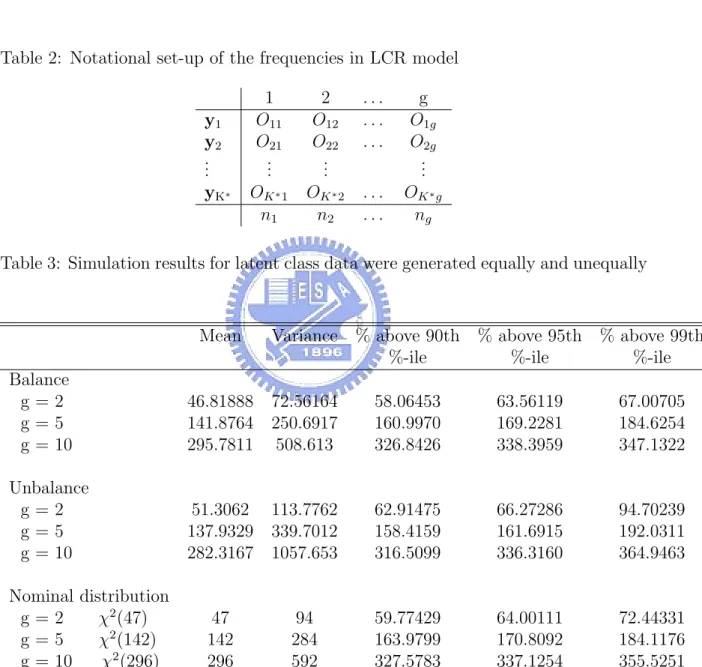
(12) Hosmer-Lemeshow statistic is a 2 × g contingency table which was obtained by defining a random variable W, where wi = j if cj−1 ≤ π î < cj , j=1, . . . , g; i=1, . . . , n. The cj ’s are known constants such that 0 = c0 < c1 < . . . < cg−1 < cg = 1. Denote the counts in the table as nkj where nkj is the frequency of occurrence of the pair (yi = k, wi = j) in the sample, k=0,1 and j=1, . . . , g. Notationally the ”observed” frequencies may tabulated as Table 1. One way of selecting the cut points c0 , . . . , cg is by defining π ˆ(1) ≤ π ˆ(2) ≤ . . . ≤ π ˆ(n) ] represents the largest as the ordered values of π ˆ and let cˆj = π ˆ([jn/g]) , where [ jn g integer less than or equal to. jn , g. j=0, 1, . . . , g. Let w î = j if cˆj−1 ≤ π ˆ < cˆj . Define. n ˆ kj as the observed frequency of the pair (yi = k, wî = j) in the sample. If Jˆj = {i : cˆj−1 ≤ π î < cˆj } then the test statistic is ) ( P P g X ˆr )]2 (n1j − r∈Jˆj π ˆr )2 [n0j − r∈Jˆj (1 − π P P + Cg = ˆr ) ˆr r∈Jˆj (1 − π r∈Jˆj π j=1. (1). and the simulation result indicated that a good approximation to the distribution of Cg is χ2 (g − 2) distributed.. 3.2. Proposed goodness-of-fit test for LCR. Similar to the Hosmer-Lemeshow goodness-of-fit, we can extend the method to our LCR model and get a test statistic by grouping our outcome variables as follows. Let the joint probability P r(Yi = yh ; φ) = Pr {(Yi1 , . . . , YiM ) = (yh1 , . . . , yhM ); φ} = πih (φ), where i = 1, . . . , N ; h = 1, . . . , K ∗ ; K ∗ =. QM m=1. (2). Km ; and φ is the vector of para-. meters. Here, the observation Yi for each i may take values {y1 , . . . , yK ∗ } where yh could be one of all possible multiple outcome for Yi , h=1, . . . , K ∗ . The basis 6.

(13) of the proposed goodness-of-fit statistic is a K ∗ × g contingency table in our LCR model. This table is obtained by defining a random variable W , where Wi = j if ˆ < cj ; j = 1, . . . , g; i = 1, . . . , N ; The cj ’s are known constants such that cj−1 ≤ πi1 (φ) ˆ is the estimate of πi1 (φ) evaluated at 0 = c0 < c1 < . . . < cg−1 < cg = 1, and πi1 (φ) the MLE of φ. Denote the counts in jth group as nj , that is, nj is the number of persons whose Wi = j. And denote Ohj is the observed frequency of occurrence of the pair Q (Yi = yh , Wi = j ) in the sample, where h = 1, . . . , K ∗ ; K ∗ = M m=1 Km ; j = 1, . . . , g. So the total observed frequencies may be tabulated as Table2. The goodness-of-fit statistic is obtained by comparing the ”observed” frequencies to ones which are ”expected” if the hypothesis of a LCR model holds. The expected frequency for the hth combination and the jth group is obtained as Ehj = P ˆ ˆ r∈Ij πrh (φ), where Ij = {i : cj−1 ≤ πi1 (φ) < cj }, j=1,2, . . . , g. Hence, the test statistic is. ∗. g K X X (Ohj − Ehj )2 . T = E hj h=1 j=1. (3). There are many methods to group the observations (that is, to define the cut points, c0 , c1 , . . . , cg ). In this thesis, we adopt the following strategy: ˆ ≤ π(2)1 (φ) ˆ ≤ . . . ≤ π(N )1 (φ)as ˆ ˆ for all i. In Define π(1)1 (φ) ordered values of πi1 (φ) other words, the cut points depend on the data and are determined so that n/g perˆ where [ jn ] represents the largest integer sons fall in each interval. Let cj = π([ jn ])1 (φ) g g. less than or equal to. 3.3. jn . g. Large sample of T. The distribution of T cannot be obtained from a straightforward application of usual theory used for χ2 goodness-of-fit test because: 7.

(14) (a). Parameter estimates are determined using likelihood functions for ”ungrouped” data. (b). The frequency, Ohj in the K ∗ × g table depend on the estimated parameters, namely the cells are random not fixed. A χ2 test under (a) were first addressed by Chernoff and Lehmann (1954) and then Watson (1959). Moore (1971) and Moore and Spruill [22] considered the distribution of the χ2 goodness of fit statistics under both (a) and (b). Their work extended the results of Watson to the case of random rectangular cells. Drust (1979) generalized these results to include random cells other than rectangles. The application of the results of Moore and Spruill [22] and Drust [21] to the problem is contained in the following theorem. Theorem 1 Let λ1 , . . . , λK ∗∗ are the non-zero or 1 eigenvalues of the matrix Σ(T ) = I − qqT − BJ −1 B T . Here, I is a K ∗ g × K ∗ g identity matrix and q is a K ∗ × g p vector with elements Phj , h = 1, . . . , K ∗ , where Phj =Pr(Y = yh , Wi = j). B is a (K ∗ × g)K ∗∗ matrix and has a general element given by √1. ∂Phj. Phj ∂ φl. , φ = (β, γ, α). J −1. is the asymptotic variance covariance matrix of the discriminant function estimates φ. Then under LCR assumptions (2), (3), and(4), the distribution of T will be asymptotically (N → ∞) χ2 (K ∗ g − g − K ∗∗ ) +. PK ∗∗ i=1. λi χ2i (1),. where 0 < λi < 1; i = 1, . . . , K ∗∗ ; K ∗∗ = (P + 1)(J − 1) + (J + L) is the total number of the parameters in the LCR model. Proof : 8. PM. m=1 (Km. − 1).

(15) The proof of the theorem follows from verifying that the regularity conditions necessary for the proof of theorem 5.1 in Moore and Spruill [22] are satisfied, see appendix.. In practice, the expected frequencies of some possible response patterns of Yi usually less than 5 even to 0. However, the χ2 approximation for the test distribution loses validity when a large number of response patterns have low expected frequencies. So we should add those response patterns which their expected frequency less than 5 to the next ones until no one take value less than 5. Therefore, we can apply our proposed goodness-of-fit method on the new response patterns and theorem1 still holds when K ∗ become the new number of response patterns after the combination.. 4 4.1. SIMULATION STUDY Data generation under the LCR model. Here, we simulated three-class LCR with five two-level measured indicators, two covariates associated with conditional probabilities, two covariates associated with latent prevalences, two, five, and ten groups (i.e., J = 3, M = 5, K1 = . . . = K5 = 2, P = L = 2, g = 2, 5, 10). The model parameters βpj can be determined through the method. For each p ∈ {0, 1, . . . , P } • randomly selected: βpj = k1 Uj , Uj ∼ U (0, 1), j = 1, . . . , (J − 1); where k1 was constants such that. PJ−1 j=1. βpj equaled the preselected total. The method. was also applied to create {γjmk , j = 1, . . . , (J − 1)} for all m, k, and {αqmk , m = 1, . . . , M ; k = 1, . . . , (Km − 1)} for all q. All (βpj , γjmk , αqmk ) pairs were generated 9.

(16) by the same method. The covariates associated with conditional probabilities (zim1 , zim2 ), m = 1, . . . , 5 and latent prevalences (xi1 , xi2 ) were generated as: zim1 ∼ Bernoulli(0.4), zim2 ∼ N ormal(0, 1), i = 1, . . . , N f or each m, xi1 ∼ Bernoulli(0.6), xi2 ∼ N ormal(0, 1), i = 1, . . . , N, all zimq and xip are mutually independent. The selected sample size was 2400, 2400, and 4800 which gave roughly 15 individuals per cell of the contingency tables for the goodness-of-fit tests with two , five and ten group. The observable Yi were then generated with 100 replications. Actually, by the common collected data the calculated expected frequencies table usually not equally distributed. For example, in evaluation functional disability, most people would task as ”not difficult” more than ” difficult”, so the number of person who tasks ”difficult” item would be very sparse. Therefore, in this thesis we simulate two situations to discuss their large sample behavior: one is equally distributed data and another is not equally distributed data. The simulation results were represented in Table3. Here, ”balance” represented the equally distributed data and χ2 (142) indicated the real χ2 distribution; ”unbalance” represented the not equally distributed data. From the results shown in Table 3, the equally distributed data was well approximated to a χ2 distribution with degree of freedom 142 and the unequally distributed data was bad approximated.. 4.2. Data generation under alternative models. This simulations considered thus far have demonstrated that the test statistic have well defined distributions under the null hypotheses that the LCR (2) model holds.. 10.

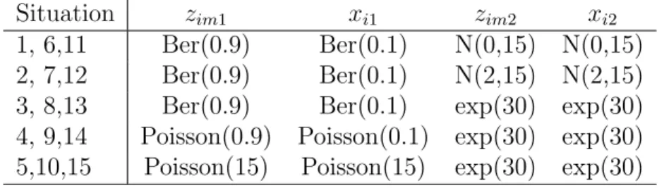
(17) To examine the power of the proposed test statistic, data were generate from the alternative models which their covariates were generated from the distributions presented in Table 4 and we considered the situations when we use a simpler model to fit the data generated from a complicated model. For situations 1-17 we use three different link functions for η to simulate. The selected sample size was 2400 and Yi0 s were generated with 100 replication for each situation. All (βpj , γjmk , αqmk ) pairs were generated by the same method as we mentioned in section 4.1. The generated data were then fitted by the LCR model stated in section 4.1. The fitted model was three-class LCR with five-two level measured indicators, two covariates associated with conditional probability, two covariates associated with latent prevalence and five groups(i.e., J=3, M=5, K1 = . . . = K5 = 2, P=L=2, g=5). Situations 1-5 used the original link function (3) we represented in section 2 and 6-10 used probit link as follows: η1 = Φ(β01 + β11 x1 + β21 x2 ); η2 = Φ(β02 + β12 x1 + β22 x2 ) × (1 − η1 ); η3 = 1 − η1 − η2 . Situation 11-15 used proportional odds model: exp(β01 + β11 x1 + β21 x2 ) ; 1 + exp(β01 + β11 x1 + β21 x2 ) exp(β02 + β11 x1 + β21 x2 ) − η1 , β02 > β01 ; = 1 + exp(β02 + β11 x1 + β21 x2 ). η1 = η2. η3 = 1 − η1 − η2 .. Situation 16, 17 used probit and proportional odds link with the original covariates. 11.

(18) For situation 18, we generated three-class LCR model with five-two level stated in section 4.1 and then fitted by the two-class LCR model with five-two levels. The test results of the above alternative models were illustrated in Table 5. The simulation results indicated that the LCR (2) did not fit the probit data particularly well, that is, the test statistic had higher power as with the probit alternative model than the other two alternative models. The test statistic did not appear to be particularly powerful in detecting the difference between the proportional odds alternative and LCR (2) models and was not powerful to detect the LCR (2) models with different covariates. For the differences between three-class and two-class LCR models, the statistic was also not sensitive. These not powerful simulation results may be due to the limiting of the replicated times, there were some difficulties to increase the replication times of our proposed models, and the way the grouping was defined or the selected alternative models were not far from the LCR model.. 5 5.1. THE SALISBURY EYE EVALUATION PROJECT Background. To illustrate the proposed diagnostic methods, we use data from Salisbuty Eye Evaluation(SEE) project. The SEE project is describe in detail in West et al. [24]. Briefly, SEE is a population-based, prospective study of risk factors for ocular pathology and of how vision affects functioning in older persons. An age- and race-stratified random sample of Salisbury, Maryland residents between the ages of 65 and 84 years was drawn from the Health Care Financing Administration (HCFA) Medicare Database. To be eligible for the study, participants had to be able to communicate in English, travel to the clinic for vision tests, and score greater than 17 on the Mini-Mental 12.

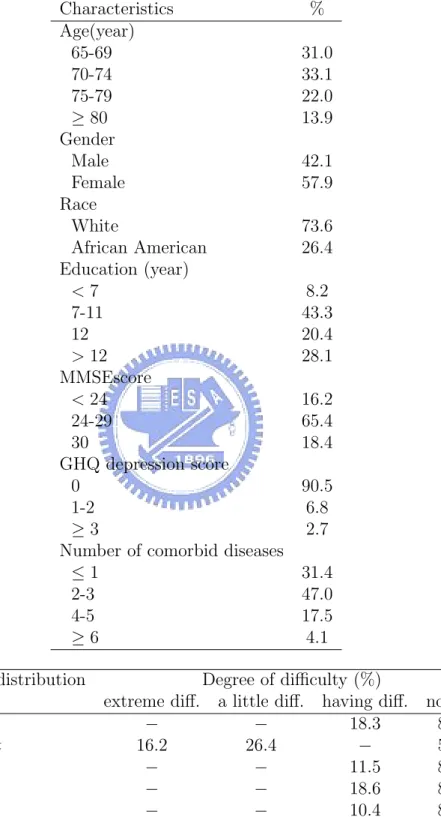
(19) State Examination (MMSE: Folstein et al. [29]). The response rate to both the home interview and clinic examination was 65%, excluding the ineligible. Twenty-five hundred and twenty persons agreed to participate in both activities. Table 6 shows the demographic characteristics of SEE participants. The analysis we report in this thesis aims to describe the association between functioning in activities that require seeing at a distance (far vision functioning) and psychophysical measures of visual impairment, adjusting for potential confounding variables. In the SEE project, visual functioning was determined using the Activities of Daily Vision Scale (ADVS) questionnaire (Mangione et al. [25], Valbuena et al. [26]). The analysis we report used selfreported difficulty doing five ADVS activities as responses: reading street signs in daylight; reading street signs at night; walking down steps during daylight; walking down steps in dim light; and watching TV. Here, we measure difficulty as a binary indicator (1=having difficulty; 2=no difficulty) for each activity, except for reading street signs at night which is measured as a three-level categorical indicator(1=extreme or moderate difficulty; 2=a little difficulty; 3=no difficulty). The hope was that, together, these five questions characterized the underlying far visual functioning. The frequency distributions of far vision subscale items are shown in Table 6. The distributions are severely skewed with most participants reporting no difficulty at all in all items. In the SEE project, visual impairment was determined using multiple psychophysical vision tests (Rubin et al. [27]). Our analysis include five test: visual acuity of both eyes at regular luminance, contrast sensitivity of the better eye, glare sensitivity of the worse eye, stereoacuity of both eyes and central visual field of both eyes. For all the measures except contrast sensitivity, a higher score indicates worse vision.. 13.

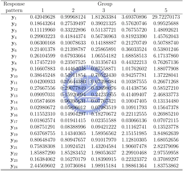
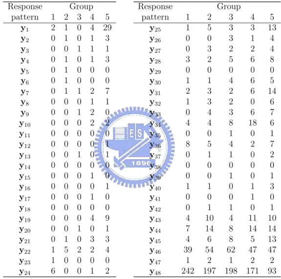
(20) 5.2. Assess the goodness of fit and analysis result. A latent class regression model (2) for self-reported visual disability was fitted as a function of visual impairment variables, the number of reported comorbid diseases, and the following personal demographic characteristics: age at clinic exam, MMSE score, years of education, indicator of being female, indicator of being AfricanAmerican, and General Health Questionnaire depression subscale score (GHQ score: Goldberg [28]). The vision and disease variables were treated as primary predictors of latent class membership (xi ), and the personal characteristics were modeled as having direct effects on measured indicators themselves within classes (zi ). The analysis was applied to the subsample of participants who rated each far vision item and also had no missing covariates(N =1641). Table 6 presented the characteristics and frequency distribution of far vision difficulty items in the SEE project, and from Table 6 we can find that the proportion of choosing no difficulty is much larger than difficulty. We started with a three-, four-, and five-class LCR model, and the hypothesis is: H0 : The fitted model explains the data well.. vs.. H1 : Not H0 .. The goodness of fit for the models began by the grouping method we proposed before. Table 7 and Table 8 displays the original contingency table for the expected and observed values when we fix a five-class model where y1 represented the response persons who self-reported as: signs-day:have difficult; signs-night: extreme difficult; steps-day: extreme difficult; steps-dim: have difficult; watch TV: have difficult; y2 represented the response persons who self-reported as: signs-day:no difficult; signsnight: extreme difficult; steps-day: extreme difficult; steps-dim: have difficult; watch TV: have difficult, and so on. We can find that some cells of the expected frequencies table are very sparse, and there are many cells take values less than 5. However, 14.

(21) the χ2 approximation for the test distribution loses validity when a large number of response patterns have low expected frequencies. So we added one row of the expected frequencies table to the next ones until no element of the row take value less than 5, and then we got a new contingency table as Table 12. Here, the first row combined the first 21 rows of the original observed frequencies table; the 2nd row combined 22th − 25th rows ,the 3rd row combined 26th − 30th rows, the 4th row combined 31th − 34th rows, the 5th row combined 35th − 38th rows ; the 6th row combined 39th−44th rows, the 7th row combined 45th−46th rows, the 8th row combined 47th− 48th rows. Table 9 and 10 are the expected and observed contingency tables after the combination. We can apply the χ2 test after the combination and the test statistic P ∗∗ 2 is 38.53494. According to Hosmer and Lemeshow, the contribution of K i=1 λi χi (1) in theorem we proposed in Section 3 is approximately that of χ2 (K ∗∗ − 2). So the distribution of our statistic is approximately to χ2 (K ∗ g − g − 2) where K ∗ is number of the response patterns after the combination, and hence in five-class LCR model of SEE project is χ2 (33). Because 38.53494 < χ20.95 (33) = 47.39988, so we can conclude that the five-class LCR model explains the data well. Similarly, Table 11 and Table 12 represents the original contingency tables of expected and observed frequencies for the four-class LCR model, and Table 15 and Table 16 represents those for three-class LCR model. For the three- and four-class LCR model, the tables also need to merge some patterns to others to let all the elements of expected table equal or larger than 5. Table 13, 14 and Table 17, 18 represents the new tables after combination for four- and three-class LCR model. The statistic for the new table of four-class LCR model was 35.92977 < χ20.95 (38) = 53.38354, so the four-class LCR model also explains the data well. The statistic for the new table of three-class LCR model was 83.83406 > χ20.95 (33) = 47.39988. Hence, 15.

(22) the data is not well explained by the three-class LCR model. From the above tests, we can conclude that the four-class LCR model is the simplest model which can well explain the data .. 6. DISCUSSION. In this thesis, we implement a latent class regression model that allows two types of covariates effects: relationships between primary predictors and responses that are mediated through the underlying variable, and direct effects of secondary covariates on the measured indicators themselves. This model is very useful in addressing scientific questions, however, the model is so complex that scientific findings are likely to be driven by the statistical assumptions rather than by the data. We develop goodnessof-fit test for assessing overall model fit. As long as operating with careful evaluation of model appropriateness, a great deal can be learned from the LCR model. The number of groups was determined by cases when we forming the contingency table. In this thesis, we selected the one such that the contingency table would not be too large or too small, and then the replicated times could be reduced in reasonable ranges. There is a lack of simulation-based investigation into the success in detecting the targeted model violations. Additional works on how various model violations appear on the proposed method is needed to identify strengths and weakness.. 16.

(23) APPENDIX Let θ be the unknown parameter in forming χ2 statistics and is estimated by θN = θN (Y1 , . . . , YN ). The parameter θ ranges over an open set Ω1 in Rg . The cells are chosen by ϕN =ϕN (Y1 , . . . , YN ). Let F (y|θ, φ) be the cdf of {Y1 , . . . , YN }. The null hypothesis is that Yi have a cdf F (y|θ). We will explore the large-sample behavior of tests for the null hypothesis under the sequences of parameter values (θ0 , φN ) ∗∗. where θ0 ∈ Ω1 and φN = φ0 + N −1/2 γ for fixed γ in RK . H0 is the special case γ = 0. We will assume that under (θ0 , φN ), ϕN − ϕ0 = oK ∗∗ (1) for some ϕ0 and θN = θ0 = ok∗∗ (1). We will suppress arguments θ, ϕ, φ whenever they take the values θ0 , ϕ0 , φ0 respectively. The resulting cells are denoted by Iσ (ϕ) , the number of Y1 , . . . , YN falling in the cell Iσ (ϕ) will be denoted by nN σ (ϕ). The cell probabilities are denoted by Pσ (θ, φ, ϕ) where σ=1, 2, . . . , K ∗∗ g. Then regular conditions of theorem 5.1 in Moore and Spruill [22] are satisfied as follows: (A1). Under (θ0 , φN ), θN −θ0 = OK ∗∗ (N −1/2 ) and ϕN −ϕ0 =oK ∗∗ (1). Every vertex y(ϕ) of every cell Iσ (ϕ) is a continuous RM -valued function of ϕ in a neighborhood of ϕ0 . (A2). For each σ, Pσ (θ, φ, ϕ) is continuous in (θ, φ, ϕ) and continuously differentiable P ∗∗ g in a neiborhood of (θ0 , φ0 , ϕ0 ). Moreover, K σ=1 Pσ = 1 and Pσ > 0 for each σ. (A3). F (y)=F (y|θ0 , φ0 ) is continuous at every vertex y(ϕ0 ) of every cell Iσ (ϕ0 ). As N → ∞, supy |F (y|φN ) − F (y)| → 0. (A4). Under (θ0 , φN ) N 1/2 (θN − θ0 ) = N −1/2. PN i=1. h(Yi , φN ) + Aγ + oK ∗∗ (1) 17.

(24) for some g × K ∗∗ matrix A and measurable function h(y, φ) from RM × RK. ∗∗. to Rg satisfying. E[h(Y, φN )|(θ0 , φN )] = 0 E[h(Y, φN )h(Y, φN )0 |(θ0 , φN )] = L(φN ) where L(φN ) is a g×g matrix converging to the finite nnd matrix L=E[h(Y)h(Y)0 ] as N → ∞. (A5). The df’s F (y|φ) possess pdf’s f (y|φ) with respect to a σ-finite dominating measure ν. As N → ∞, f (y|φN ) → f (y|φ0 ) and h(y, φN ) → h(y) a.e. (ν). (A6). N. 1/2. (θˆN − θ0 ) = N −1/2. N X. J −1. i=1. ∂ log f (Yi |φN ) + J −1 J12 γ + oK ∗∗ (1). ∂θ. P Here θˆN maximizes N i=1 log f (Yi |θ), J is the information matrix for F (y|θ) at θ0 ,. ·µ J =E. ∂ log f ∂θ. ¶µ. ∂ log f ∂θ. ¶0 ¸ ,. J12 is the m × p matrix ·µ J12 = E. ∂ log f ∂θ. ¶µ. ∂ log f ∂φ. ¶0 ¸ .. (A7). Let VN (θ, φ, ϕ) be an M-vector and it’s σth component is nN σ (ϕ) − N Pσ (θ, φ, ϕ) . [N Pσ (θ, , φ, ϕ)]1/2 18.

(25) Then N 1/2 (θ¯ − θ0 ) = (B 0 B)−1 B 0 VN (φN ) + (B 0 B)−1 B 0 B12 γ + oK ∗∗ (1), P ∗∗ ∗ where θ¯ maximizes K σ=1 nN σ (ϕ) log Pσ (θ, ϕN ) and the K × g matrix B12 has (i, j)th entry −1/2. Pi. ∂Pi . ∂φj. (A8). g ≤ K ∗ g and the matrix with entries ∂Pi /∂θj has rank g. (A9). A7 holds, so that θ¯N satisfies A4 with A = (B 0 B)−1 B 0 B12 and h(y) = (B 0 B)−1 B 0 W (y), where χσ (y) indicator function of Iσ (ϕ0 ) and W (y) the K ∗ g vector with σth 1/2. component [χσ (y) − Pσ ]/Pσ . (A10). log f (y|θ, φ) is differentiable with respect to (θ, φ) at (θ0 , φ0 ). The matrix J is pd and J12 is finite. (∂/∂θ)F (y|θ) may be evaluated by differentiating f (y|θ) under the integral sign for all y and θ = θ0 . (A11). A7 holds, so that θˆN satisfies A4 with A = J −1 J12 and h(y) = J −1 (∂ log f (y|θ, φ)/∂θ)|θ0 ,φ . 0. (A12). J − B 0 B is pd.. 19.

(26) REFERENCES 1. Green BF. A general solution of the latent class model of latent structure analysis and latent profile analysis. P sychometrika 1951; 16: 151-166. 2. Lazarsfeld PF, Henry NW. Latent Structure Analysis. New York: HoughtonMifflin, 1968. 3. Goodman LA. Exploratory latent structure analysis using both identifiable and unidentifiable models. Biometrika 1974; 61: 215-231. 4. Haberman SJ. Log-linear models for frequency tables derived by indirect observation: maximum likelihood equations. Annualsof Statistics 1974; 2: 911-924. 5. Haberman SJ. Analysis of Qualitative Data. V ol. 2 : N ew Developments. New York: Academic Press, 1979. 6. Dayton CM, Macready GB. Concomitant-variable latent-class models. Journal of the American Statistical Association. 1988; 83: 173-178. 7. Formann AK. Linear logistic latent class analysis for polytomous data. Journal of the American Statistical Association. 1992; 87: 476-486. 8. Bandeen-Roche K, Miglioretti DL, Zeger SL, Rathouz PJ. Latent variable regression for multiple discrete outcomes. Journal of the American Statistical Association. 1997; 92: 1375-1386. 9. Muthén B, Shendden K. Finite mixture modeling with mixture outcomes using EM algorithm. Biometrics 1999, 55: 463-469.. 20.

(27) 10. Melton B, Liang K-Y, Pulver AE. Extended latent class approach to the study of familial/sporadic forms of a disease: its application to the study of the heterogeneity of schizophrenia. Genetic Epidemiology 1994; 11: 311-327. 11. Huang GH, Bandeen-Roche L. Latent variable regression with covariate effects on underlying and measured variables: an approach of analyzing multiple polytomous surrogates. Submitted for publication. 12. Batholomew DJ. Latent Variable Models and Factor Analysis. London: Charles Griffin & Co. Ltd, 1987. 13. Titterington DM, Smith AFM, Makov UE. Statistical Analysis of Finite Mixture Distributions. Chichester, U.K.: Wiley, 1985. 14. McCullagh P, Nelder JA. Generalized Linear Models, 2nd edition. London: Chapman and Hall, 1989. 15. Agresti A. Analysis of Categorical Data. New York: J. Wiley and Sons, 1984. 16. Bandeen-Roche K, Huang GH, Munoz B, Rnbin GS. Determination of risk factor associations with questionnaire outcomes: a methods case study. American Journal of Epidemiology 1999; 150: 1165-1178. 17. Demster AP, Laird NM, Rubin DB. Maximum likelihood from incomplete data via the EM algorithm. Journal of the Royal Statistical Society, Series B 1977; 39: 1-38. 18. Hosmer, D. W., Lemeshow, S. Goodness-of-fit Tests for the Multiple Logistic Regression Model. Communications in Statistics, 1980; A10: 1043-1069.. 21.

(28) 19. Lemeshow S., Hosmer D.W.. The Use of Goodness-of-fit Statistics in the Development of Logistic Regression Models. American Journal of Epidemiology, 1982; 115: 92-106. 20. Hosmer DW, Lemeshow S. Applied Logistic Regression. New York: John Wiley & Sons. 21. Drust MC. Donsker. Vapnik-Chervonenkis classes and chi-square tests of fit with random cells, 1980; Unpublished doctoral dissertation, Department of Mathematics, M.I.T., Cambridge, MA. 22. Moore D.S., Spruill M.C. Unified Large-sample Theory of General Chi-squared Statistics for Tests of Fit. Annals of Statistics, 1975; 3: 599-616. 23. Huang GH. Selecting the number of classes under latent class regression models: a factor analysis analogous approach. Submitted for publication. 24. West SK, Munoz B, Rubin GS, Schein OD, Bandeen-Roche K, Zeger SL, German PS, Fried LP. Function and visual impairment in a population-based study of older adults: SEE project. Investigative Ophthalmology and Visual Science 1997; 38: 72-82. 25. Mangione CM, Phillips RS, Seddon JM, Lawrence MG, Cook EF, Dailey R, Goldman L. Development of the ”activities of daily vision” scale: a measurement of visual functional status. Medical Care 1992; 30: 1111-1126. 26. Valbuena M, Bandeen-Roche K, Rubin GS, Munoz B, West SK, SEE project team. Self-reported assessment of visual functioning in a population based setting. Investigative Ophthalmology and Visual Science 1999; 40: 280-288. 22.

(29) 27. Rubin GS, West SK, Munoz B, Bandeen-Roche K, Zeger SL, Scgein O, Fried LP. A comprehensive assessment of visual impairment in an older American population: SEE study. Investigative Ophthalmology and Visual Science 1997; 38: 557-568. 28. Goldberg D. GHQ The Selection of Psychiatric Illness by Questionnaire. London: Oxford University Press, 1972. 29. Folstein MF, Folstein SE, McHgh PR. Mini-mental state: a practical method for grading the cognitive state of patients for the clinician. Journal of Psychiatric Research1975; 12: 189.. 23.

(30) Table 1: Notational set-up of the frequencies in logistic regression model y=0 y=1 Total. 1 n01 n11 n•1. 2 n02 n12 n•2. ... ... ... .... g n0g n1g n•g. Total n0 n1 n. Table 2: Notational set-up of the frequencies in LCR model 1 O11 O21 .. .. 2 O12 O22 .. .. ... ... .... g O1g O2g .. .. OK ∗ 1 n1. OK ∗ 2 n2. ... .... OK ∗ g ng. y1 y2 .. . yK∗. Table 3: Simulation results for latent class data were generated equally and unequally. Mean. Variance % above 90th %-ile. % above 95th %-ile. % above 99th %-ile. Balance g=2 g=5 g = 10. 46.81888 141.8764 295.7811. 72.56164 250.6917 508.613. 58.06453 160.9970 326.8426. 63.56119 169.2281 338.3959. 67.00705 184.6254 347.1322. Unbalance g=2 g=5 g = 10. 51.3062 113.7762 137.9329 339.7012 282.3167 1057.653. 62.91475 158.4159 316.5099. 66.27286 161.6915 336.3160. 94.70239 192.0311 364.9463. 59.77429 163.9799 327.5783. 64.00111 170.8092 337.1254. 72.44331 184.1176 355.5251. Nominal distribution g=2 χ2 (47) g=5 χ2 (142) g = 10 χ2 (296). 47 142 296. 94 284 592. 24.

(31) Table 4: Generated covariates for alternative models Situation 1, 6,11 2, 7,12 3, 8,13 4, 9,14 5,10,15. zim1 xi1 zim2 xi2 Ber(0.9) Ber(0.1) N(0,15) N(0,15) Ber(0.9) Ber(0.1) N(2,15) N(2,15) Ber(0.9) Ber(0.1) exp(30) exp(30) Poisson(0.9) Poisson(0.1) exp(30) exp(30) Poisson(15) Poisson(15) exp(30) exp(30). Table 5: Simulation results for situations 1-18 Situation 1 2 3 4 5. mean 140.1411 140.9580 141.0234 139.8990 139.4221. variance 329.5329 311.0997 304.7142 290.2688 258.986. α=0.05 power 0.07 0.04 0.09 0.07 0.06. 6 7 8 9 10. 140.6912 304.635 141.3010 254.3497 142.0696 288.4761 140.6636 291.4900 141.1024 294.3013. 0.06 0.03 0.07 0.08 0.1. 11 12 13 14 15. 140.8594 140.3471 144.2373 140.1092 140.0726. 265.5376 270.9357 274.0058 267.8568 250.0764. 0.02 0.04 0.09 0.06 0.03. 16. 140.7425. 241.9495. 0.07. 17. 141.3161. 247.0320. 0.06. 18. 144.4393. 269.5813. 0.09. 25.

(32) Table 6: Demographic characteristics and frequency distribution of far vision difficulty items: SEE project (N=2520) Characteristics Age(year) 65-69 70-74 75-79 ≥ 80 Gender Male Female Race White African American Education (year) <7 7-11 12 > 12 MMSEscore < 24 24-29 30 GHQ depression score 0 1-2 ≥3 Number of comorbid diseases ≤1 2-3 4-5 ≥6. % 31.0 33.1 22.0 13.9 42.1 57.9 73.6 26.4 8.2 43.3 20.4 28.1 16.2 65.4 18.4 90.5 6.8 2.7 31.4 47.0 17.5 4.1. Frequency distribution Degree of difficulty (%) Activities extreme diff. a little diff. having diff. signs-day − − 18.3 signs-night 16.2 26.4 − step-day − − 11.5 steps-dim − − 18.6 watch T V − − 10.4. 26. no diff. 81.7 57.4 88.5 81.4 89.6.

(33) Table 7: Contingency table of the expected frequencies for the five-class LCR model of SEE project Response pattern y1 y2 y3 y4 y5 y6 y7 y8 y9 y10 y11 y12 y13 y14 y15 y16 y17 y18 y19 y20 y21 y22 y23 y24. 1 0.42049628 0.18643264 0.11119960 0.29903223 0.06300168 0.21401378 0.26104599 0.17457210 0.16607883 0.38645248 0.04200933 0.27667556 0.09097031 0.05874608 0.02980672 0.11552310 0.01862574 0.08751291 0.63768755 0.80648470 0.75838308 1.85887290 0.16384062 2.44569602. 2 0.99968124 0.27539497 0.33222896 0.41844374 0.10078633 0.21398787 0.67933664 0.23507525 0.44464038 0.54911854 0.05644380 0.29077849 0.15926094 0.06395631 0.05806012 0.14904297 0.01941415 0.08388996 1.14340365 0.80947657 1.10924521 1.85283452 0.16270179 2.10736084. Group 3 1.81263384 0.39021325 0.51137721 0.56736963 0.14188887 0.25865891 1.06554182 0.31356743 0.67558871 0.70523430 0.07398084 0.32698076 0.24235955 0.07767421 0.07983519 0.18270672 0.02351588 0.09421222 1.58956562 0.91017970 1.43204584 1.98053637 0.18390915 1.98915184. 27. 4 5 3.69370896 29.72270173 0.57620746 0.99525688 0.76755720 1.48092621 0.81923390 1.45762043 0.21270749 0.50788740 0.36033524 0.53801246 1.68858513 6.17137860 0.44322213 0.76267136 1.01762602 1.88077908 0.94257781 1.37228041 0.10387555 0.26671268 0.41438756 0.58527210 0.41409407 2.46833773 0.10047405 0.13134480 0.10911793 0.15647378 0.22112555 0.26985210 0.03066136 0.07072115 0.11162741 0.13523778 2.15151985 3.84862639 1.12810305 1.68052656 1.90607478 2.82379096 2.29910468 2.97559958 0.22323372 0.37089297 1.98861364 1.83753862.

(34) Response pattern y25 y26 y27 y28 y29 y30 y31 y32 y33 y34 y35 y36 y37 y38 y39 y40 y41 y42 y43 y44 y45 y46 y47 y48. Group 1 2 3 4 0.54042227 1.73156563 2.81586975 4.15098379 1.09828562 1.56198456 2.15043059 3.01754843 0.60144036 1.60463972 2.40415869 3.31413678 1.79694626 2.93859969 4.04802492 5.24541618 0.32890596 0.47399871 0.63245982 0.85320599 1.26454454 1.44735271 1.82453947 2.38028614 0.85062691 2.65441513 4.26555237 6.09161241 1.15130224 1.69965419 2.26762283 2.99815672 0.91258949 2.22682930 3.28979151 4.52216227 3.94518861 6.69430173 8.72773722 10.55980526 0.22046238 0.27909237 0.35011903 0.45957534 4.37773774 5.29408268 5.97981629 6.82891761 0.13023080 0.30000679 0.43644729 0.59433628 0.34588037 0.42898907 0.53640686 0.66122105 0.16235453 0.28784858 0.38270096 0.49530050 0.74436805 1.48056945 1.95359229 2.17974196 0.09688252 0.09316940 0.10517277 0.12963315 0.53769469 0.72674833 0.89919330 1.02940472 3.45079913 5.78162334 7.70581607 9.90671502 7.54361584 10.63312563 11.80221091 12.53484838 4.26883963 5.88123132 7.22737492 9.06883811 40.06027971 54.67193447 56.43316835 54.42342720 1.12298026 1.40463204 1.51398265 1.64979597 242.77446186 205.38904195 184.61908324 163.18115618. 28. 5 10.27999890 4.44128717 4.71608401 7.40559661 1.13644414 3.02789299 10.728768035 4.51704113 7.06590127 12.50051423 0.94005296 7.61818812 1.12270149 0.77008515 0.62961065 2.25137670 0.15425575 1.09668809 13.73782580 13.67550209 12.62221788 43.95310627 2.36773250 99.73068633.

(35) Table 8: Contingency table of the observed frequencies for the five-class LCR model of SEE project Response pattern 1 y1 1 y2 0 y3 0 y4 1 y5 1 y6 0 y7 0 y8 0 y9 0 y10 0 y11 0 y12 0 y13 0 y14 0 y15 0 y16 0 y17 0 y18 0 y19 0 y20 0 y21 0 y22 3 y23 1 y24 4. 2 2 1 1 0 0 1 1 0 0 0 0 0 0 0 0 0 0 0 0 0 0 3 0 2. Group 3 4 5 1 2 30 0 2 2 0 1 1 0 1 3 0 0 0 0 0 0 1 1 8 0 1 1 1 2 0 0 2 2 0 0 0 0 0 1 1 0 1 0 0 0 0 1 0 0 1 0 0 1 0 0 0 0 0 4 9 1 0 1 1 4 2 4 1 3 0 0 0 0 2 1. Response pattern y25 y26 y27 y28 y29 y30 y31 y32 y33 y34 y35 y36 y37 y38 y39 y40 y41 y42 y43 y44 y45 y46 y47 y48. 29. Group 1 2 3 1 4 3 0 0 2 0 2 4 2 3 4 0 0 0 2 0 3 1 5 1 2 1 3 0 4 5 6 3 7 0 0 1 5 8 3 0 1 1 0 0 0 0 0 1 1 1 0 0 0 0 0 2 0 5 9 2 7 13 9 4 7 6 38 55 62 1 2 1 242 197 200. 4 3 2 1 7 0 5 5 0 6 18 0 3 0 0 0 0 1 0 11 13 6 47 1 173. 5 14 4 4 8 0 7 15 6 5 6 1 7 2 0 1 4 0 1 12 15 13 47 3 89.

(36) Table 9: Contingency table of the expected frequencies for the five-class LCR model of SEE project after combining the rows which were less than 5 Response pattern y10 y20 y30 y40 y50 y60 y70 y80. Group 1 2 3 4 5 5.20475070 8.19166609 11.47513052 17.21282251 57.32641060 5.00883181 5.85446277 6.96946711 8.66193583 15.46403006 5.09012273 8.02657539 11.05961349 14.81059352 20.72730491 6.85970724 13.27520034 18.55070393 24.17173667 34.81222466 5.07431128 6.30217091 7.30278947 8.54405028 10.45102772 12.53571477 19.00308472 22.84868631 26.27564373 31.54525907 44.32911934 60.55316579 63.66054327 63.49226532 56.57532415 243.89744211 206.79367399 186.13306590 164.83095215 102.09841883. Table 10: Contingency table of the observed frequencies for the five-class LCR model of SEE project after combining the rows of expected frequencies table which were less than 5 Response pattern y10 y20 y30 y40 y50 y60 y70 y80. Group 1 2 3 2 7 6 9 8 8 3 6 15 9 13 13 5 8 6 13 26 10 42 64 66 245 196 204. 30. 4 22 5 15 31 4 26 54 171. 5 62 19 21 33 9 33 59 93.

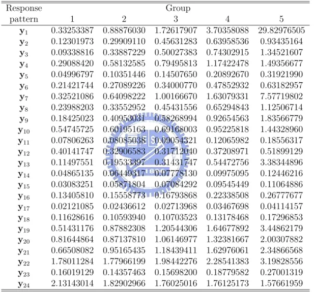
(37) Table 11: Contingency table of the expected frequencies for the four-class LCR model of SEE project Response pattern y1 y2 y3 y4 y5 y6 y7 y8 y9 y10 y11 y12 y13 y14 y15 y16 y17 y18 y19 y20 y21 y22 y23 y24. 1 0.33253387 0.12301973 0.09338816 0.29088420 0.04996797 0.21421744 0.32521086 0.23988203 0.18425023 0.54745725 0.07806263 0.40141747 0.11497551 0.04865135 0.03083251 0.13405810 0.02121085 0.11628616 0.51431176 0.81644864 0.66508082 1.78011284 0.16019129 2.13143014. 2 0.88876030 0.29909110 0.33887229 0.58132585 0.10351446 0.27089226 0.64098222 0.33552952 0.40953031 0.60195163 0.08085038 0.32906583 0.19533397 0.06449317 0.05871804 0.15558773 0.02436612 0.10593940 0.87882308 0.87137810 0.95165435 1.77966199 0.14357463 1.82902966. Group 3 1.72617907 0.45631283 0.50027383 0.79495813 0.14507650 0.34000770 1.00166670 0.45431556 0.58268994 0.69168003 0.09054321 0.31712040 0.31431747 0.07778130 0.07084292 0.16793868 0.02713968 0.10703523 1.20544306 1.06146977 1.18439411 1.98442276 0.15698200 1.76025016. 31. 4 5 3.70358088 29.82976505 0.63958536 0.93435164 0.74302915 1.34521607 1.17422478 1.49356677 0.20892670 0.31921990 0.47852932 0.63182957 1.63079331 7.57719802 0.65294843 1.12506714 0.92654563 1.83566779 0.95225818 1.44328960 0.12065982 0.18556317 0.37208971 0.51899129 0.54472756 3.38344896 0.09975095 0.12446216 0.09545449 0.11064886 0.22338508 0.26777677 0.03467698 0.04114157 0.13178468 0.17296853 1.64677892 3.44862179 1.32381667 2.00307882 1.62976061 2.34866568 2.28541383 3.19828556 0.18779582 0.27001319 1.76125173 1.57661959.

(38) Response pattern y25 y26 y27 y28 y29 y30 y31 y32 y33 y34 y35 y36 y37 y38 y39 y40 y41 y42 y43 y44 y45 y46 y47 y48. Group 1 2 3 4 5 0.35008546 1.35659933 2.20562021 3.20297809 9.50318998 0.74971719 1.70878508 2.52018322 3.28079288 4.22723731 0.54646183 1.89329414 2.68646415 3.50791726 4.35527884 1.73592421 3.20052301 4.26688494 5.78982934 6.94303779 0.30625298 0.58797149 0.78197613 1.00356313 1.20707350 1.31455773 1.52752317 1.89741854 2.48843086 3.22194006 0.82709725 2.42881286 3.78911593 5.58826854 11.03174882 1.63680029 2.31386936 3.11301295 4.16099641 6.48235890 1.23046411 2.67246263 3.68526124 5.21172681 7.75399850 3.89644176 5.06612099 5.97139292 7.33903102 9.86007980 0.50905302 0.51441872 0.56835118 0.69374280 0.97892556 4.89962474 6.35564147 6.95464367 7.35305454 7.59107044 0.10765676 0.22050313 0.29985853 0.39987288 1.09156276 0.30021062 0.38517418 0.46821588 0.57362767 0.75073846 0.18316997 0.32686049 0.38314876 0.47461805 0.51148020 0.82563371 1.01004948 1.15725911 1.44404737 1.77213408 0.13074221 0.14082310 0.15350743 0.18209205 0.21774938 0.85496731 1.04591266 1.22574937 1.45074646 1.76654086 3.09297696 5.32888010 6.96298252 8.91537464 11.97127840 7.69814344 9.91887907 11.55472314 12.48776853 15.04856313 4.80917652 6.59156023 7.89861846 9.89917022 12.64121238 40.52719260 57.36985264 58.14678568 56.11497384 44.71831148 1.44144168 1.50706755 1.56976274 1.64623074 1.95424084 240.6123 202.5895 184.5202 163.2234 99.21479. 32.

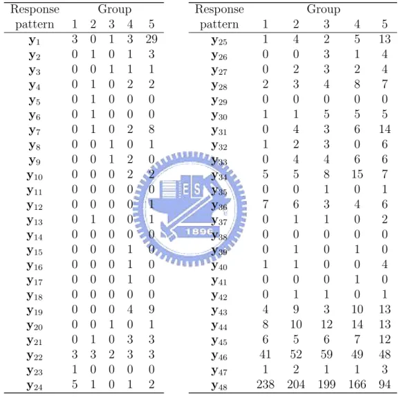
(39) Table 12: Contingency table of the observed frequencies for the four-class LCR model of SEE project Response pattern 1 y1 3 y2 0 y3 0 y4 0 y5 0 y6 0 y7 0 y8 0 y9 0 y10 0 y11 0 y12 0 y13 0 y14 0 y15 0 y16 0 y17 0 y18 0 y19 0 y20 0 y21 0 y22 3 y23 1 y24 5. 2 0 1 0 1 1 1 1 0 0 0 0 0 1 0 0 0 0 0 0 0 1 3 0 1. Group 3 4 5 1 3 29 0 1 3 1 1 1 0 2 2 0 0 0 0 0 0 0 2 8 1 0 1 1 2 0 0 2 2 0 0 0 0 0 1 0 0 1 0 0 0 0 1 0 0 1 0 0 1 0 0 0 0 0 4 9 1 0 1 0 3 3 2 3 3 0 0 0 0 1 2. Response pattern y25 y26 y27 y28 y29 y30 y31 y32 y33 y34 y35 y36 y37 y38 y39 y40 y41 y42 y43 y44 y45 y46 y47 y48. 33. Group 1 2 3 1 4 2 0 0 3 0 2 3 2 3 4 0 0 0 1 1 5 0 4 3 1 2 3 0 4 4 5 5 8 0 0 1 7 6 3 0 1 1 0 0 0 0 1 0 1 1 0 0 0 0 0 1 1 4 9 3 8 10 12 6 5 6 41 52 59 1 2 1 238 204 199. 4 5 1 2 8 0 5 6 0 6 15 0 4 0 0 1 0 1 0 10 14 7 49 1 166. 5 13 4 4 7 0 5 14 6 6 7 1 6 2 0 0 4 0 1 13 13 12 48 3 94.

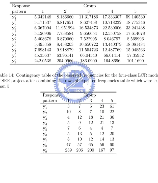
(40) Table 13: Contingency table of the expected frequencies for the four-class LCR model of SEE project after combining the rows which were less than 5 Response pattern y10 y20 y30 y40 y50 y60 y70 y80 y90. Group 1 2 3 5.342148 8.186660 11.317186 5.171537 6.817651 8.627458 6.367094 11.951994 16.534873 5.126906 7.738584 9.656654 5.408678 6.870060 7.522995 5.495358 8.458203 10.650722 7.698143 9.918879 11.554723 45.33637 63.96141 66.04540 242.0538 204.0966 186.0900. 4 17.333307 10.718232 22.539006 12.550758 8.046797 13.440379 12.487769 66.01414 164.8696. 5 59.140539 18.775346 33.241438 17.614078 8.569996 18.081484 15.048563 57.35952 101.1690. Table 14: Contingency table of the observed frequencies for the four-class LCR model of SEE project after combining the rows of expected frequencies table which were less than 5 Response pattern y10 y20 y30 y40 y50 y60 y70 y80 y90. Group 1 2 3 3 7 5 10 8 7 4 12 18 5 9 12 7 6 4 5 13 5 8 10 12 47 57 65 239 206 200. 34. 4 23 10 21 21 4 12 14 56 167. 5 61 22 36 13 7 20 13 60 97.

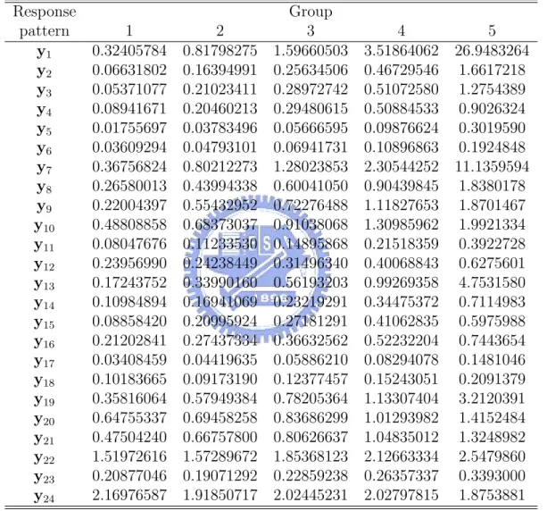
(41) Table 15: Contingency table of the expected frequencies for the three-class LCR model of SEE project Response pattern y1 y2 y3 y4 y5 y6 y7 y8 y9 y10 y11 y12 y13 y14 y15 y16 y17 y18 y19 y20 y21 y22 y23 y24. 1 0.32405784 0.06631802 0.05371077 0.08941671 0.01755697 0.03609294 0.36756824 0.26580013 0.22004397 0.48808858 0.08047676 0.23956990 0.17243752 0.10984894 0.08858420 0.21202841 0.03408459 0.10183665 0.35816064 0.64755337 0.47504240 1.51972616 0.20877046 2.16976587. 2 0.81798275 0.16394991 0.21023411 0.20460213 0.03783496 0.04793101 0.80212273 0.43994338 0.55432952 0.68373037 0.11233530 0.24238449 0.33990160 0.16941069 0.20995924 0.27437334 0.04419635 0.09173190 0.57949384 0.69458258 0.66757800 1.57289672 0.19071292 1.91850717. Group 3 1.59660503 0.25634506 0.28972742 0.29480615 0.05666595 0.06941731 1.28023853 0.60041050 0.72276488 0.91038068 0.14895868 0.31496340 0.56193203 0.23219291 0.27181291 0.36632562 0.05886210 0.12377457 0.78205364 0.83686299 0.80626637 1.85368123 0.22859238 2.02445231. 35. 4 5 3.51864062 26.9483264 0.46729546 1.6617218 0.51072580 1.2754389 0.50884533 0.9026324 0.09876624 0.3019590 0.10896863 0.1924848 2.30544252 11.1359594 0.90439845 1.8380178 1.11827653 1.8701467 1.30985962 1.9921334 0.21518359 0.3922728 0.40068843 0.6275601 0.99269358 4.7531580 0.34475372 0.7114983 0.41062835 0.5975988 0.52232204 0.7443654 0.08294078 0.1481046 0.15243051 0.2091379 1.13307404 3.2120391 1.01293982 1.4152484 1.04835012 1.3248982 2.12663334 2.5479860 0.26357337 0.3393000 2.02797815 1.8753881.

(42) Response pattern y25 y26 y27 y28 y29 y30 y31 y32 y33 y34 y35 y36 y37 y38 y39 y40 y41 y42 y43 y44 y45 y46 y47 y48. Group 1 2 3 4 5 0.34618763 1.24966160 1.87897444 3.09709248 8.8822582 0.41998864 0.99242695 1.45233677 2.22456248 3.5973526 0.41622423 1.44323607 2.03034090 3.06023537 4.9028305 0.72897336 1.43692742 2.04567192 3.10515507 4.6623652 0.12262888 0.24403947 0.33893170 0.49490892 0.7610699 0.30753832 0.37095790 0.50106892 0.71078433 1.0286178 1.18058453 3.07399241 4.12491926 5.88679677 9.7491025 2.29924369 3.47367270 4.49002260 6.02125844 8.2445501 1.82860813 4.00924885 5.20820143 7.10716757 9.4369980 4.58041870 6.34962584 7.82626714 10.06252554 13.2375753 0.69721477 0.88501791 1.09892286 1.39996599 1.8116868 4.41785669 5.52047584 6.00410260 6.72210412 7.5024807 0.44533935 1.08344795 1.43421384 1.98575668 3.2063911 0.88417430 1.22496464 1.57919151 2.07845882 2.7209311 0.71366107 1.46137652 1.88348772 2.52648921 3.2242573 1.74918913 2.07598775 2.64761156 3.41781722 4.3899174 0.27952619 0.32699495 0.40740409 0.50711334 0.6259024 0.97502204 0.91612645 1.10491131 1.27840021 1.4815578 2.26397726 3.44103394 4.06401867 4.96421676 5.9669476 8.32469842 10.80300523 11.37814988 12.17386995 11.9393512 4.12665914 5.31976653 6.16510334 7.26372174 8.1203980 41.14785545 56.72699335 55.20611448 54.27339198 42.0665447 2.29350821 2.33661203 2.47253783 2.57161914 2.5536178 239.1044 202.1637 187.9694 163.4812 101.8699. 36.

(43) Table 16: Contingency table of the observed frequencies for the three-class LCR model of SEE project Response pattern 1 y1 2 y2 0 y3 0 y4 0 y5 0 y6 0 y7 0 y8 0 y9 0 y10 0 y11 0 y12 0 y13 0 y14 0 y15 0 y16 0 y17 0 y18 0 y19 0 y20 0 y21 0 y22 1 y23 1 y24 6. 2 1 1 0 1 1 1 1 0 0 0 0 0 0 0 0 0 0 0 0 0 1 5 0 0. Group 3 4 5 0 4 29 0 1 3 1 1 1 0 1 3 0 0 0 0 0 0 1 2 7 0 1 1 1 2 0 0 2 2 0 0 0 0 0 1 1 0 1 0 0 0 0 1 0 0 0 1 0 1 0 0 0 0 0 4 9 1 0 1 0 3 3 2 2 4 0 0 0 0 1 2. Response pattern y25 y26 y27 y28 y29 y30 y31 y32 y33 y34 y35 y36 y37 y38 y39 y40 y41 y42 y43 y44 y45 y46 y47 y48. 37. Group 1 2 3 1 5 3 0 0 3 0 3 2 3 2 5 0 0 0 1 1 4 2 3 2 1 3 2 0 4 3 4 4 8 0 0 1 8 5 4 0 1 1 0 0 0 0 0 1 1 1 0 0 0 0 0 1 1 4 10 4 7 14 8 4 6 8 39 54 62 1 2 1 242 197 198. 4 3 1 2 6 0 6 6 0 6 18 0 2 0 0 0 1 1 0 11 14 5 47 2 171. 5 13 4 4 8 0 5 14 6 7 6 1 7 2 0 1 3 0 1 10 14 13 47 2 93.

(44) Table 17: Contingency table of the expected frequencies for the three-class LCR model of SEE project after combining the rows which were less than 5 Response pattern y10 y20 y30 y40 y50 y60 y70 y80. Group 1 2 3 5.968004 8.961505 12.435048 5.900662 10.920462 14.625289 8.708271 13.832547 17.524491 5.115071 6.405494 7.103025 5.046912 7.088898 9.056820 10.58868 14.24404 15.44217 43.12666 59.31977 68.16510 241.3979 204.5003 190.4419. 4 5 19.293858 64.802688 20.871087 35.798285 23.190952 30.919123 8.122070 9.314167 11.794035 15.648957 17.13809 17.90630 54.26372 55.12040 166.0528 104.4235. Table 18: Contingency table of the observed frequencies for the three-class LCR model of SEE project after combining the rows of expected frequencies table which were less than 5 Response pattern y10 y20 y30 y40 y50 y60 y70 y80 y90. Group 1 2 3 3 12 7 14 14 19 5 11 13 8 5 5 1 3 3 11 24 12 43 60 70 47 57 65 243 199 199. 38. 4 25 25 24 2 2 25 52 56 173. 5 66 50 19 8 7 24 60 60 95.

(45)