Time-based OVSF Code Allocation Schemes in WCDMA Systems

全文

(1)Name of the Workshop: Workshop of Computer Networks Title of the Paper: Time-based OVSF Code Allocation Schemes in WCDMA Systems Abstract:. In the third generation mobile communication systems, orthogonal variable spreading factor (OVSF) are used for spreading codes. Efficient allocation of codes for users is an important issue in radio resource management. In this paper, we address the impacts of remaining time factor on OVSF code allocation in WCDMA systems. We also propose two time-based allocation schemes for code assignment and reassignment. Simulation results show that the time-based allocation schemes have better performance on probability of call blocking and codes utilization.. Authors: Chia-Mei Chen,. Ming-Tzung Hsieh,. Department of Information Management, National Sun Yat-Sen Univeristy, Kaohsuing, Taiwan 801, R.O.C. Email: [email protected]. Department of International Trade, Kao-Yuan Institute of Technology, Kaohsiung, Taiwan 821, R.O.C Email:[email protected]. and, Sheng-Tzong Cheng, Department of Computer Science and Information Engineering, National Cheng Kong University, Tainan, Taiwan 701, R.O.C Email:[email protected]. Contact Author: Prof. Chia-Mei Chen. Keywords:. OVSF code assignment, WCDMA, Wireless Communications, and multimedia applications. 1.

(2) Time-based OVSF Code Allocation Schemes in WCDMA Systems1 Chia-Mei Chen,. Ming-Tzung Hsieh,. Department of Information Management, National Sun Yat-Sen Univeristy, Kaohsuing, Taiwan 801, R.O.C. Email: [email protected]. Department of International Trade, Kao-Yuan Institute of Technology, Kaohsiung, Taiwan 821, R.O.C Email:[email protected]. and, Sheng-Tzong Cheng, Department of Computer Science and Information Engineering, National Cheng Kong University, Tainan, Taiwan 701, R.O.C Email:[email protected]. Abstract In the third generation mobile communication systems, orthogonal variable spreading factor (OVSF) are used for spreading codes. Efficient allocation of codes for users is an important issue in radio resource management. In this paper, we address the impacts of remaining time factor on OVSF code allocation in WCDMA systems. We also propose two time-based allocation schemes for code assignment and reassignment. Simulation results show that the time-based allocation schemes have better performance on probability of call blocking and codes utilization.. 1. Introduction The key features of the third generation mobile communication systems are high data rate and variable data rate for different requirements. To satisfy those requirements, wideband code division multiple access (W-CDMA) technology has emerged as a candidate for radio access in Universal Mobile Telecommunication Systems (UMTS)[3]. In W-CDMA, orthogonal variable spreading codes (OVSF) are used as spreading and channelization codes [1,2]. The use of OVSF codes allows the spreading factors to be changed for variable bit rate, moreover, the orthogonality between different spreading codes of different lengths would be preserved. The generation of OVSF codes can be represented by a tree-structure. To preserve the orthogonality, some restrictions are posed in code allocation in a code tree. Under these constrains, how to allocate the codes effectively will be an important issue. The objective. 1. This work is supported by Institute of Information Industry under the contract of 91-C-33. 2.

(3) of codes allocation is to support as many users as possible, that is, to make the best utilization and reduce the call blocking probability. When a new call arrives, we have to assign a new OVSF code such that the code tree to be most flexible for future request. After a period of time, some codes are released and the code tree may be too fragmental for high bit rate request to be assigned. In this situation, we have to rearrange the code tree to reserve a large free space for future request. Many different schemes are proposed for codes assignment and codes reassignment. However, all of the known schemes are space-based, that is, the main factor considered is the space factor in the code tree. The space-based schemes make the code tree as compact as possible. Consequently, the free space is large enough to accept more requests in the future. On the other hand, we observe that the duration time of most multimedia applications can be obtained apriori. The remaining time factor of an occupied code may have significant impact on future code assignment and reassignment costs. In this paper, we proposed two time-based allocation schemes that take the remaining time of each call as main factor for codes assignment and reassignment. The rest of the paper is organized as follows. In section 2, we describe the structure of OVSF code trees and features of OVSF codes. Besides, we address the issues on OVSF code allocation. In section 3, we describe the problems of OVSF code allocation with remain time factor in multimedia applications, and introduce our proposed allocation schemes. In section 4, we present the simulation results. Finally, we conclude our work in section 5.. 2. Issues in Code Allocation 2.1 OVSF codes In CDMA systems, channelization codes are used to separate the downlink connections to different users within one cell. The channelization codes of WCDMA are based on the orthogonal variable spreading factor technique. The use of OVSF codes allows the spreading factor to be changed for variable bit rate requirements. It preserves the orthogonality between different spreading codes for different users.. 3.

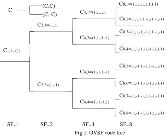
(4) C. C8,1=(1,1,1,1,1,1,1,1). (C,C) (C,-C). C4,1=(1,1,1,1) C8,2=(1,1,1,1,-1,-1,-1,-1). C2,1=(1,1) C8,3=(1,1,-1,-1,1,1,-1,-1) C4,2=(1,1,-1,-1) C8,4=(1,1,-1,-1,-1,-1,1,1). C1,1=(1). C8,5=(1,-1,1,-1,1,-1,1,-1) C4,3=(1,-1,1,-1) C8,6=(1,-1,1,-1,-1,1,-1,1). C2,2=(1,-1). C8,7=(1,-1,-1,1,1,-1,-1,1) C4,4=(1,-1,-1,1) C8,8=(1,-1,-1,1,-1,1,1,-1) SF=1. SF=2. SF=4 SF=8 Fig 1. OVSF code tree. The OVSF codes can be represented using a tree structure as shown in Fig 1 [4]. Each code in the code tree is denoted as CSF,code number, where SF indicates spreading factor and the code number is a sequence number ranging from 1 to SF. The code with smaller SF value provides the higher data bit rate. For example, if the data rate of a code in the layer with SF=8 is R, the codes in the layer with SF=4 and SF =2 will be 2R and 4R respectively. Codes in the same layer are orthogonal, meanwhile, codes in the different layers are also orthogonal if they don’t have the ancestor-descendant relationship. To make sure all assigned codes are orthogonal, there are certain restrictions on code allocation in the code tree. A code can be assigned to a new call if and only if no other code on the path from the specified code to the root of the tree or in the sub-tree below the specified code is assigned. In other words, codes with ancestor-descendant relationships should not to be assigned at the same time. For example, in Fig1, if code C4,1 is used, the ancestor codes C2,1 ,C1,1 and the descendant codes C8,1, C8,2 can’t be assigned until C4,1 is released.. 2.2 Issues in codes allocation Codes allocation deals with the problem of how different codes are assigned to different connections. Because of the constrains on code tree, the strategy of codes allocation would play an important role for code utilization. In this section, we address the issues in codes allocations. Consider a new call arrives and requests for a code for data bit rate R. If there is no free 4.

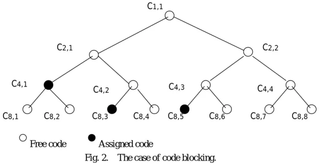
(5) code for rate R, the call will be rejected, and causes a call blocking. On the other side, if there are many free codes for rate R, we have to pick a code from those candidates and assign it to the call. Different choices may cause different utilizations for the future arriving call. We call this problem as code assignment problem or code placement problem. In code assignment, the objective is to support as many users as possible. The system shall provide the best code utilization and the least call blocking probability. Upon the arrival of a new request for the data bit rate R, we may rearrange the occupied codes in the code tree to aggregate the free capacity for the new request, if (1) there is no available single code for this request, and (2) the total free capacity of the code tree is enough for the new call. We call this problem as the code reassignment problem or code replacement problem. In code reassignment problem, the objective is to minimize the reassignment cost, that is, to minimize the number of codes to be reassigned. C1,1. C2,1. C4,1 C8,1. C2,2. C4,3. C4,2 C8,2 Free code. C8,3. C8,4. C8,5. C4,4 C8,6. C8,7. C8,8. Assigned code Fig. 2. The case of code blocking.. In Fig.2, we illustrate a code blocking situation. If the data rate for the leaves in the code tree is R, the data rates for SF=8, 4, 2, 1 are R, 2R, 4R and 8R respectively. The total capacity is 8R. The codes C4,1, C8,3 and C8,5 are occupied by previous calls, the free capacity of the code tree is 4R. If a new call arrives and requests for data rate 8R, the call is rejected and causes a call blocking due to the shortness of capacity. If a new call arrives and requests for data rate R, C8,4, C8,6, C8,7 and C8,8 are available candidates. However, different selection strategies result in different situations. Suppose we select C8,7 or C8,8 for this request, later on, another new call arrives and requests for data rate 2R. The call will be rejected because of no available free code. In the contrast, if we choose C8,4 or C8,6 for this request, C4,4 is available for incoming request of 2R. In this case, C8,4 or C8,6 is the better choice than C8,7 or C8,8. If a new call arrives and requests for data rate 4R, the call will be rejected because of no available code even free capacity is enough. Suppose we reassign 5.

(6) the code C8,5 to C8,4 such that the code C2,2 is available for this request, the call blocking will be eliminated. In the similar situations, we can reassign code C4,1 to C4,4, and code C8,3 to C8,6, and release code C2,1 for the new request. However, in the later case, two codes have to be reassigned with hihger cost than the former case.. 3. QoS Support for Code Allocation 3.1 Related Work In the literature, many code allocation schemes were proposed [6, 7]. The main goal of those schemes is to make the assigned codes as compact as possible, and aggregate the free codes together to accommodate future coming high data rate calls. In [5], a dynamic code allocation (DCA) scheme is proposed for code reassignment. This DCA scheme is based on code pattern search, and has minimum reassignment cost. All the work is space-based scheme, that is, code allocation is based on the space factor of the code tree. In the third generation mobile communication systems, multimedia applications for different quality of services (QoS) guarantee are supported. In most multimedia applications, such as video on demand, video conferencing, downloading music files etc., time duration of the requests can be obtained apriori. Thus, the remaining time of each code occupied in the code tree is known. The remaining time factor of an occupied code may have significant impact on future code assignment and reassignment costs. If we arrange the near remaining time codes together, and as the time goes by, the codes with near remaining time codes would be released together. There may release a large free space to accept new calls. It would support more users and reduce the call blocking probability. In the next section, we address the proposed time-based allocation schemes.. 3.2. Time-based allocation schemes. We propose time-based allocation schemes in which time is the main factor to be considered. We define the remaining time of a code as the time different between the current time and the time when the code is released. Namely, the remaining time of a code indicates the residual duration of an occupied code before it is released. Initially, remaining time of all nodes are 0’s. When a call arrives and to be accepted, an OVSF code is assigned to the call. The remaining time of this code is the duration time of the call request. As time goes by, the remaining time is decreased, and becomes 0 when the time is up and the code is released. A branch is a complete binary subtree of the code tree. The remaining time of a branch is defined as the maximum remaining time of all occupied codes in the branch. All nodes except for leaf nodes are root nodes of some branches. The proposed schemes take into account the remaining time of the branches 6.

(7) to allocate OVSF codes. In Fig.3(a), the remaining time of all nodes are 0 at the beginning. Later, a new request comes for data rate of R with request duration time of 20 time units, code C8,2 is assigned by the system as illustrated in Fig 3(b). The parents nodes C4,1 inherits the remaining time of 20 time units, that is, the branch code tree with root node C4,1 will be fully empty after 20 time units. Similarly, codes C2,1 and C1,1 have remaining time of 20 time units. After 5 time units, the remaining time of codes C8,2 , C4,1 and C1,1 are decreased to 15 time units. At the same time, suppose a new call requests for data rate of 2R with request time duration of 40 time units, and assigned with code C4,2. From the definition of the remaining time of a branch, the remaining time of branch code tree with root node C2,1 is replaced by the maximum item between children nodes C4,1 and C4,2. The remaining time of branch code tree with root node C2,1 will be updated to 40 time units, that is, all nodes in the branch code tree will be released after 40 time units. Similarly, branch code tree with root node C1,1 will be updated to 40 time units. C1,1 Rt=0. C2,1 Rt=0 C4,1 Rt=0 C8,1 Rt=0. C2,2 Rt=0 C4,2 Rt=0. C8,2 Rt=0. C8,3 Rt=0. C4,3 Rt=0 C8,4 Rt=0. C8,5 Rt=0. C4,4 Rt=0 C8,6 Rt=0. C8,7 Rt=0. C8,8 Rt=0. (a) Initially, the remaining time of all nodes are 0’s. C1,1 Rt=20. C2,1 Rt=20 C4,1 Rt=20 C8,1 Rt=0. C2,2 Rt=0 C4,2 Rt=0. C8,2 Rt=20. C8,3 Rt=0. C4,3 Rt=0 C8,4 Rt=0. C8,5 Rt=0. C4,4 Rt=0 C8,6 Rt=0. (b) A new call request for data rate R and with duration time 20. 7. C8,7 Rt=0. C8,8 Rt=0.

(8) C1,1 Rt=40. C2,1 Rt=40 C4,1 Rt=15 C8,1 Rt=0. C2,2 Rt=0 C4,2 Rt=40. C8,2 Rt=15. C8,3 Rt=0. C4,3 Rt=0 C8,4 Rt=0. C8,5 Rt=0. C4,4 Rt=0 C8,6 Rt=0. C8,7 Rt=0. C8,8 Rt=0. (c) 5 time units later, a new call request for data rate 2R and with duration time 40 time units. Fig. 3.. An illustration of remaining time of code tree.. In Fig. 4, we illustrate the impact of remaining time factor on future code assignment and code reassignment. Continued on Fig. 3, codes C4,3 and C8,2 are occupied with remaining time of 80 and 15 time units respectively. Consider the case in which a new call request for data rate 2R with duration time of 70 time units. As we can see, the selection of different candidate codes, C4,2 and C4,4, could result in different situations as shown in Fig.4(b) and Fig.4(c) respectively. After 15 time units, code C8,2 is released. Observably, C4,4 is better than C4,2 because of supporting higher data rate request after 15 time units. In the case without code reassignment, it reduces the call blocking probability by supporting higher data rate request. In the other case with code reassignment, it reduces the number of moved codes.. 3.3. Code assignment schemes. As we mentioned in previous subsection, remaining time is an important factor of codes assignment and reassignment. Therefore, we proposed two time-based code assignment schemes, Maximum Remaining Time First (MF) and Nearest Sibling Remaining Time First (NSF). These time-based allocation schemes are constrained on the request duration time be known in advance. We describe these two schemes below:. Maximum Remaining Time First (MF) In this scheme, we select the candidate codes by comparing the remaining time of their parents nodes, and pick the maximum one for the assignment of the new call. The main idea of this scheme is that the request duration time of the new call will be absorbed by the maximum remaining time of the parent code. The code tree may be less fragmental after a 8.

(9) period of time. The algorithm is described as follows. (1) While a new call arrives, check if the available codes satisfy its requirement. If so, go to step 2, else reject the call. (2) If there are more candidate codes in the code tree, select the one whose parent code has the maximum remaining time of a branch. If the comparison results in a tie, we compare the remaining time of the upper layer ancestor node till the maximum one is found. The special case is that the ancestor nodes are the roots of the same branch. We may select the one randomly or the leftmost one. (3) Assign the selected code to the call. For example, suppose the current status of code tree is shown as Fig.5. If a new call request for data rate 2R and duration time 30 time units. There are three candidates for this call, C8,3, C8,6 and C8,7. According to the MF scheme, the branch remaining time of parent nodes of these three codes are 20, 65 and 10 time units respectively. Code C8,6 with remaining time 65 time units is the maximum. Thus, we assign code C8,6 to the C1,1 Rt=80. C2,1 Rt=15 C4,1 Rt=15 C8,1 Rt=0. C2,2 Rt=80 C4,2 Rt=0. C8,2 Rt=15. C8,3 Rt=0. C4,3 Rt=80 C8,4 Rt=0. C8,5 Rt=0. C4,4 Rt=0 C8,6 Rt=0. C8,7 Rt=0. C8,8 Rt=0. (a) The initial status of code tree. Codes C4,3 and C8,2 are occupied with remaining time 80 and 15 time units respectively.. C1,1 Rt=65. C2,1 Rt=55 C4,1 Rt=0 C8,1 Rt=0. C2,2 Rt=65 C4,2 Rt=55. C8,2 Rt=0. C8,3 Rt=0. C4,3 Rt=65 C8,4 Rt=0. C8,5 Rt=0. C4,4 Rt=0 C8,6 Rt=0. C8,7 Rt=0. C8,8 Rt=0. (b) C4,2 is allocated with duration time 70 time units. After 15 time units later, code C8,2 is released. The code tree supports maximum of data rate 2R request. 9.

(10) C1,1 Rt=65. C2,1 Rt=0 C4,1 Rt=0 C8,1 Rt=0. C2,2 Rt=65 C4,2 Rt=0. C8,2 Rt=0. C8,3 Rt=0. C4,3 Rt=65 C8,4 Rt=0. C8,5 Rt=0. C4,4 Rt=55 C8,6 Rt=0. C8,7 Rt=0. C8,8 Rt=0. (c) C4,4 is allocated with duration time 70 time units. After 15 time units later, code C8,2 is released. The code tree supports maximum of data rate 4R request.. Fig. 4 The impact of remaining time factor on future code assignment and reassignment. new call. After 20 time units, the branches with root code C4,2 and C4,4 would be free . In this case, C8,6 are superior to C8,3 and C8,7 observably.. Nearest Sibling Remaining Time First (NSF) In this scheme, we select the candidate codes by comparing the remaining time of their sibling nodes, and pick the one who has the closest value to the request duration time, in other words, the sibling with minimum difference. For aggregation, we put the nodes with similar remaining time together. Since they will be released at the similar time, a larger and more compact space will be available to support higher data rate request. It also could reduce the probability of call blocking. The algorithm is described as follows. (1) While a new call arrives, check if the available codes satisfy its requirement. If so, go to step 2, else reject the call. (2) If there are more candidate codes in the code tree, select the one whose sibling code (or parent code) has the least difference from the request duration time of the new call. If the comparison results in a tie, we compare the remaining time of the upper layer ancestor node till the least one is found. The special case that the ancestor nodes are the roots of the same branch. We may select the one randomly or the leftmost one. (3) Assign the selected code to the call. Refer to the same example in Fig.5, if a new call request for data rate of R and duration time of 18 time units. There are many candidates for this call, C16,5, C16,6, C16,8, C16,11, C16,12, C16,13, C16,14 and C16,16. According to the NSF scheme, we compare the remaining time of sibling nodes of the candidates. The remaining time of sibling code of a free code is equal to the remaining time of its parent code. Thus, we. 10.

(11) C1,1. Rt=80. C2,1. C2,2. Rt=80. Rt=65. C4,1. C4,2. Rt=80. C8,1. Rt=40. C4,3. Rt=20. C8,2. C8,3. Rt=80. C8,4. Rt=0. C4,4. Rt=65. C8,5. Rt=20. Rt=10. C8,6. C8,7. Rt=0. Rt=65. C8,8. Rt=0. Rt=10. C16,1 C16,2 C16,3 C16,4 C16,5 C16,6 C16,7 C16,8 C16,9 C16,10 C16,11 C16,12 C16,13 C16,14 C16,15 C16,16 Rt=15 Rt=40 Rt=0 0 0. Rt=0. Rt=0. Rt=0. Rt=20 Rt=0. Rt=0. Rt=0. Rt=0. Rt=0. Rt=0. Rt=0. Rt=10 Rt=0. Fig 5. An example of code assignment and reassignment.. would get the same results by comparing the parent nodes of the candidates. In this case, code C16,7, the sibling of code C16,8 with remaining time 20 time units is the nearest from the new request duration time 18 time units. Code C16,8 is chosen for the new call.. 3.4. Code reassignment schemes. Multiple operations of code assignment and code release may result in a code tree with fragmental codes. Fragmental codes lead to low utilization because of no available code for new request even the total capacity is enough to support. In this situation, we have to rearrange the code tree to aggregate the used codes together. Thus, a bigger code is available to support higher data rate request. However, the cost of rearranging the code tree is the number of code movements. It should be as least as possible. In [2], a dynamic code allocation (DCA) scheme is proposed using code pattern search. The code pattern of a branch is defined in terms of A/B, where A is the total number of occupied descendant codes and B denotes their occupied capacity. A branch with code pattern A/B has a smaller moving cost than a branch with code pattern C/D if (A < C) or (A = C and B < D). This scheme states which code should be reassigned to ensure minimum moving cost, however, where to reassign is not addressed. In fact, where to place the reassigned codes may have a significant impact on future utilization. In this subsection, we propose the time-based code reassignment schemes based on the DCA scheme. The algorithm is stated as follows. (1) While a new call arrives, check if the request data rate is within the available system capacity. If so, go to step 2, otherwise reject the call. (2) If there are one or more available codes in the code tree, select the code using MF or 11.

(12) MSDF schemes we proposed before. If no available code exists, that is, we have to move some occupied codes. Go to step3. (3) Apply the DCA scheme to search the minimum cost branch where the root code supports the request rate of the new call. From the root to the lower layer, all the occupied codes in the branch need to be reassigned. (4) Once a minimum cost branch is empty. Assign the root code of the branch to the new call. Where to place the reassigned code is based on the code assignment schemes we proposed before (MF, NSF). That is, go to step 2 to treat it as a new call request its data rate, and trigger another round of this scheme. For example, suppose the status of code tree is shown as Fig.5. If a new call request for data rate 4R and duration time 50 time units. At the first, check the available system capacity. The total capacity is 16R, and 8R in used, thus 8R is available. The new request for data rate 4R is within the system capacity. However, there is no available code that supports data rate 4R. We apply the DCA scheme to search the minimum cost branch. The code C4,2 and C4,4 has the same code pattern and the minimum moving cost. Based on the MF scheme, we prefer to allocate the new call to code C4,2. Before the allocation, we have to reassign the occupied code, such as C16,7, in the branch. We treat it as a new call request for data rate R and duration time 20 time units, thus apply the algorithm again. There are five available positions for C16,7 to reassign, that is, C16,11, C16,12, C16,13, C16,14, C16,16. According to the MF scheme, C16,16 is chose and reallocated. Finally, assign code C4,2 to the new call and terminate the process. The example for NSF reassignment scheme can be processed in a similar way.. 4 Simulation Results In this section, we develop a simulation model to evaluate the performance of the proposed schemes. To contrast with the effective of time-based allocation schemes, we also compare with two common space-based allocation schemes random and leftmost schemes [7].. 4.1 System parameters The system parameters of this simulation are stated as below: Input parameter: λ: new call arrival rate. The inter-arrival time of new request is assumed to be exponential distributed with mean 1/λ. μ: new call request duration rate. The call duration is assumed to be exponential distributed with mean 1/μ. q : λ/μ, the ratio of inter arrival rate to the duration rate. To specify the performance of different traffic loads, we classify three traffic loads as shown in Table. 1. for. 12.

(13) example, in light load case, the proportion of coming call with different q is 5:3:1. q : λ/μ. 0.5. 1. 1.5. 3. 5. 8. 15. 20. Light load. 5. 3. 1. Average load. 1. 1. 1. Heavy load. 1. 3. 5. 25. Table 1 Different traffic load in terms of q Maximum SF: 128 Possible request data rate: R, 2R, 4R, 8R, 16R, 32R Output parameters: For code assignment without reassignment, we consider the call blocking probability. In the others, for code assignment with reassignment, we focus on the number of new calls that have to be reassigned and the total number of moved codes.. 4.2 Simulation results The simulation results are obtained from the average of 10 runs, each run contain 50000 calls. To compare with common space-based allocation schemes, the random and leftmost schemes [7] are tested also. The random scheme randomly selects an available code to assign to new request. The leftmost scheme selects the leftmost available one in the code tree to assign to a new call. In fact, the leftmost scheme always aggregates the used codes in the left part and reserves the free codes at the right part future higher request rate. For code assignment without reassignment, we expect the code tree to support as many users as possible. Reduce the probability of call blocking and increase the utilization of code systems. The simulation results are shown as Table 2(a) and Fig. 6(a). The NSF scheme seems to have better performance because of less blocking probability. For code assignment with reassignment, the probability of call blocking will be reduced absolutely. However, we concerns with the reassign cost. The probability of reassign codes for a new call will be expected to be low. At the same time, the total number of code reassignment will be expected to be small. Table 2(b) and Fig. 6(b) depict the probability of the code tree needs to be rearranged for a new call, that is, the probability of no available code for a new call even the system capacity is enough. It occurs because of the code tree is. light load average load heavy load. random leftmost MF NSF 0.0403 0.0115 0.0115 0.0110 0.1184 0.0614 0.0614 0.0596 0.1895 0.1336 0.1336 0.1191 13.

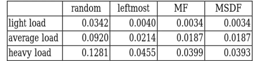
(14) (a) The call blocking probability of code assignment without reassignment.. light load average load heavy load. random leftmost 0.0342 0.0040 0.0920 0.0214 0.1281 0.0455. MF 0.0034 0.0187 0.0399. MSDF 0.0034 0.0187 0.0393. (b) The probability of the code tree needs to be rearranged for a new call.. light load average load heavy load. random 2031 6853 11317. left 251 1510 3469. MF 222 1384 3171. MSDF 223 1390 3169. (c) The total number of code assignments Table 2 Simulation results for different schemes. blocking probability. 0.2000 0.1500. random leftmost. 0.1000. MF NSF. 0.0500 0.0000 light load. average load. heavy load. traffic load. (a) The call blocking probability of code assignment without reassignment.. code reassignment probability. 0.1400 0.1200 random left MF MSDF. 0.1000 0.0800 0.0600 0.0400 0.0200 0.0000 light load. average load traffic load. 14. heavy load.

(15) (b) The probability of the code tree needs to be rearranged for a new call.. number of reassigned codes. 12000 10000 8000 6000 4000. random. 2000. left. 0. MF light load. average load. heavy load. MSDF. traffic load. (c) The total number of code assignments Fig.6 The simulation results too fragmental to accept a new call for higher data rate. Time-based allocation schemes keep the code tree less fragmental than the other two schemes. Finally, in Table 2(c) and Fig 6.(c), the total number of code reassignment indicates the cost of moving occupied codes to accommodate a new call. Time-based allocation schemes spend the less cost, and it is more significant as traffic load increases.. 5 Conclusions In this paper, we address the impacts of remaining time factor on OVSF code allocation in WCDMA. We also propose two time-based allocation schemes. In those schemes, remaining time of the codes are the main factor to be considered for allocating a new call. We arrange the code tree by remaining time of occupied codes, the codes with similar remaining time aggregate. They may be released together at the nearest time, thus, a larger free capacity is available to accept a new call with higher rate. Based on the simulation results, we find that the time-based allocation schemes we proposed have better performance than common space-based allocation schemes.. References [1] 3GPP Technical Specification 25.213, Spreading and Modulation (FDD) [2] 3GPP Technical Specification 25.922, Radio Resource Management Strategies. [3] H. Holma and A. Toskala. WCDMA for UMTS. John Wiley & Sons, 2000 [4] F. Adachi, M. Sawahashi and K.Okawa, “Tree-structured generation of orthogonal spreading codes with different lengths for forward link of DS-CDMA mobile radio”, Electronics Letters, Vol. 33, No. 1, pp.27-28, January 1997. [5] T. Minn and K. Y. Siu, “Dynamic Assignment of Orthogonal Variable Spreading 15.

(16) Factor Codes in W-CDMA”, IEEE Journal on Selected Areas in Communications, Vol.18, No. 8, pp.1429 – 1440, August 2000. [6] W. T. Chen, Y. P. Wu and H. C. Hsiao “A Novel Code Assignmnet Scheme for W-CDMA Systems”, IEEE VTS [7] Y. C. Tseng and C. M. Chao, “Code placement and Replacement Strategies for Wideband CDMA OVSF Code Tree Management”, The 8th Mobile Computing Workshop, pp.188-195, March 2002.. 16.

(17)