Stability Analysis of Neural-Network Large-scale Systems

全文

(1)Stability Analysis of Neural-Network Large-scale Systems Zhen-Yuan Chen, Cheng-Wu Chen ∗ and Wei-Ling Chiang2 1. 2. 1. Department of Marine Environment and Engineering, National Sun Yat-Sen University, Kaohsiung, R.O.C.. 2. Department of Civil Engineering, National Central University, Chung-Li, Taiwan, R.O.C.. Abstract This paper is concerned with the stability problem of a neural network (NN) large-scale system which consists of a few interconnected subsystems represented by NN models. First, the dynamics of each NN model is converted into LDI (linear differential inclusion) representation. Subsequently, based on the LDI representations, a stability criterion in terms of Lyapunov's direct method is derived to guarantee the asymptotic stability of NN large-scale systems. Finally, a numerical example with simulations is given to illustrate the results. Key words— Large-scale system, neural network.. I. Introduction A great number of today’s problems are brought about by present-day technology and societal and environmental processes which are highly complex, large in dimension, and stochastic by nature. The field of large-scale systems exists so widely that covers either the fundamental theory of modeling, optimization, and control or certain particular aspects and applications. In addition, large-scale systems analysis, design, and control theory has attained considerable maturity and sophistication and is receiving increasing attention from theorists and practitioners, for both its methodological attraction and its important real-life applications [1]. In real systems, the large-scale systems include electric power systems, nuclear reactors, aerospace systems, large electric networks, economic systems, process control systems, chemical and petroleum industries, different types of societal systems, and ecological systems. Such systems consist of a number of interdependent subsystems which serve particular functions, share resources, and are governed by a set of interrelated goals and constraints [2]. Recently, many ∗ Author to whom all correspondence should be addressed (s8322004@cc.ncu.edu.tw). 1.

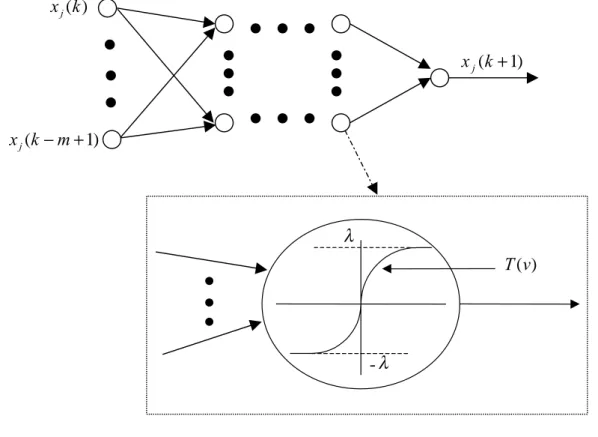
(2) approaches have been used to investigate the stability and stabilization of large-scale systems, as proposed in the literature [3-6]. During the past several years, neural network (NN)-based modeling has become an active research field because of its unique merits in solving complex nonlinear system identification and control problems. Neural networks are composed of simple elements operating in parallel. These elements are inspired by biological nervous systems. Then, we can train a neural network to represent a particular function by adjusting the weights between elements. However, the stability analysis of nonlinear large-scale systems via NN model-based control is so difficult that rare researches were reported. Therefore, the LDI representation is employed in this study to deal with the stability analysis of nonlinear large-scale systems. In this paper, we consider an NN large-scale system composed of a set of subsystems with interconnections. One critical property of control systems is stability and considerable reports have been issued in the literature on the stability problem of NN dynamic systems (see [7-9] and the references therein). However, as far as we know, the stability problem of NN large-scale systems remains unresolved. Hence, a stability criterion in terms of Lyapunov's direct method is derived to guarantee the asymptotic stability of NN large-scale systems. This paper may be viewed as a generalization of the approach of [8] to the stability analysis of NN large-scale systems. This study is organized as follows. First, the system description is presented. Next, based on Lyapunov approach, a stability criterion is derived to guarantee the asymptotic stability of NN large-scale systems. Finally, a numerical example with simulations is given to demonstrate the results, followed by conclusions. II. System description and stability analysis. Consider a neural-network (NN) large-scale system N which consists of J subsystems with interconnections. In addition, the jth isolated NN subsystem (without interconnection) of N, shown in Fig. 1, has S j ( j = 1, 2,⋅ ⋅ ⋅, J ) layers with R τ ( τ = 1, 2,⋅ ⋅ ⋅, S j ) neurons for each layer, in which x j (k ) ~ x j (k − m + 1) are the state variables. It is assumed that v is the net input and all the transfer functions Τ (v) of units in the jth isolated NN subsystem are described by the. 2.

(3) following sigmoid function:      2  Τ (v ) = λ  − 1 ,  1 + exp − v    ς      . (1). where ς , λ > 0 are the parameters associated with the sigmoid function. In addition, we need to introduce some additional notations to specify these layers. The superscripts are used for identifying the layers. Specifically, we append the number of the layer as a superscript to the names of the variables. Thus, the weight matrix for the nth layer is written as W n , and the transfer function vector of the nth layer can be defined as. [. ]. Ψ τ (v) ≡ T1 (v) T2 (v) ⋅ ⋅ ⋅ TR τ (v) , T. τ = 1, 2, ⋅ ⋅⋅, S j. where Tl (v) ( l = 1, 2,⋅ ⋅ ⋅, R τ ) are the transfer functions associated with Ψ τ (v) . Then the final output of the jth isolated NN subsystem can be inferred as follows: x j (k ) x j (k + 1). x j (k − m + 1). λ Τ (v). -λ. S. S. x j (k + 1) = Ψ j (W j Ψ where T. −2 S j −1Fig. S1. TheS jjth j −1. (W. Ψ. ⋅ ⋅ ⋅ ⋅ ⋅ ⋅ Ψ 2NN Ψ 1 (W 1 X j (k ))) ⋅ ⋅ ⋅ ⋅ ⋅ ⋅))) , (isolated (W 2subsystem.. [. ]. X j (k ) = x j (k ) x j (k + 1) ⋅ ⋅ ⋅ x j (k − m + 1) .. 3. (2).

(4) Next, a linear differential inclusion (LDI) system in the state-space representation is introduced and it can be described as follows [10] : rj. A( z (k )) = ∑ hi ( z (k )) Ai ,. y (k + 1) = A( z (k )) y (k ),. (3). i =1. where r j is a positive integer, z (k ) is a vector signifying the dependence of hi (⋅) on its the elements and y (k ) = [y1 (k ). y 2 (k ) ... y m (k )] . Furthermore, it is assumed that T. rj. ∑ hi ( z (k )) = 1 .. hi ( z (k )) ≥ 0 ,. i =1. From the properties of LDI, without loss of generality, we can use hi (k ) instead of hi ( z (k )) . Then, the procedure of the conversion of the jth isolated NN subsystem (2) into an LDI representation is given as follows [9]. First, it can be found obviously that the output of transfer function Τ (v) satisfies g1 v ≤ Τ ( v ) ≤ g 2 v ,. v≥0. g 2 v ≤ Τ ( v ) ≤ g1 v ,. v<0. where g1 and g 2 are the minimum value and the maximum value of the derivative of Τ (v) , and they are given in the following: d Τ (v )  =0  g 1 = min v dv g (T ) =   g 2 = max d Τ (v) = λ v  dv 2ς. (4) ⋅. Subsequently, given transfer function vectors Ψ τ (v ) and net input vectors v τ , the min-max matrix G (v τ , Ψ τ ) is defined as follows: G (vτ , Ψ τ ) = diag ( g (Τ l )) ,. l = 1, 2 , ..., R τ .. (5). Moreover, based on the interpolation method and Eq. (2), we can obtain 2. 2. S. S. S. S. S. 2. 2. x j (k + 1) = [ ∑ ⋅ ⋅ ⋅ ∑ h Sj (k ) ⋅ ⋅ ⋅ h Sj (k )G (v j , Ψ j )(W j [⋅ ⋅ ⋅[ ∑ ⋅ ⋅ ⋅ ∑ hq22 (k ) ⋅ ⋅ ⋅ hq22 (k ) q q S S q1 =1 q j. j. RS. j. =1. j. j. 1. RS. q12 =1 qR2 2 =1. j. 1. R2. 2. 2. G (v 2 , Ψ 2 )(W 2 [ ∑ ⋅ ⋅ ⋅ ∑ h1q1 (k ) ⋅ ⋅ ⋅ h1q1 (k )G (v1 , Ψ 1 )(W 1 X j (k ))])] ⋅ ⋅⋅])] 1 q11 =1 q1 1 =1. R1. R. S. S. S. S. = ∑ ⋅ ⋅ ⋅ ∑ hv Sj (k ) ⋅ ⋅ ⋅ hv11 (k )G (v j , Ψ j )W j ⋅ ⋅ ⋅ G (v1 , Ψ1 )W 1 X j (k ) v. Sj. j. v1. = ∑ hv j (k ) Av j (W , Ψ ) X j (k ) ,. (6). vj. where. 4.

(5) h1τ (k ), h2τ (k ) ∈ [0, 1], 2. 2. q1τ =1. q τ τ =1. 2. ∑ hqτ (k ) = 1 , τ l. qlτ =1. ∑ hvτ (k ) = ∑ ⋅ ⋅ ⋅ ∑ hqτ (k ) ⋅ ⋅ ⋅ hqτ (k ), vτ. τ. τ 1. τ Rτ. R. S. S. Av j (W , Ψ ) ≡ G (v j , Ψ j )W. Sj. ⋅ ⋅ ⋅ G (v1 , Ψ 1 )W 1 ,. S ∑ hv (k ) ≡ ∑ ⋅ ⋅ ⋅∑ hv (k ) ⋅ ⋅ ⋅ hv1 (k ) = 1 , vj. j. v. Sj. j Sj. v. 1. 1. hv j (k ) ≥ 0 . According to Eq. (3), the dynamics of the jth isolated NN subsystem (6) can be rewritten as the following LDI representation: rj. X j (k + 1) = ∑ hij (k ) Aij X j (k ) , i =1. hij (k ) ≥ 0 ,. where. (7). rj. ∑ hij (k ) = 1 ,. i =1. Aij (k ) is a constant matrix with appropriate dimension associated with Av (W , Ψ ) and rj is a positive integer. Based on the analysis above, the jth NN subsystem N j with interconnections can be described as follows: rj  X ( k + 1 ) = hij (k ) Aij X j (k ) + φ j (k ) ∑  j i =1  N j : J  φ j (k ) = ∑ Cnj X n (k ), n =1  n≠ j. (8a) (8b). where Cnj is the interconnection matrix between the nth and jth subsystems. In the following, a stability criterion is proposed to guarantee the asymptotic stability of the NN large-scale system N. Prior to examination of asymptotic stability, a useful concept is given below. Lemma 1 [11] : For any matrices A and B with appropriate dimension, we have AT B + B T A ≤ κAT A + κ −1 B T B. where κ is a positive constant. Theorem 1: The NN large-scale system N is asymptotically stable, if there exists positive constant κ is chosen to satisfy. 5.

(6) ( I ) λˆij = λ M (Qij ) + α ijn < 0 ,. λˆifj = λ M (Qifj ) + 2α ijn < 0 ,. for. i = 1, 2, L, r j ; j = 1, 2,⋅ ⋅ ⋅, J. (9a). for. i < f < r j ; j = 1, 2,⋅ ⋅ ⋅, J. (9b). or  λˆ1 j 1 / 2λˆ12 j  λˆ2 j 1 / 2λˆ12 j ( II )  M M  1 / 2λˆ1r j j 1 / 2λˆ2 r j j. L 1 / 2λˆ1r j j   L 1 / 2λˆ2 r j j  <0 M M   L λˆr j j . j = 1, 2,⋅ ⋅ ⋅, J. for. (10). where J ~ α ijn = λ M (Qijn ) + η j , η j = ∑ ( J − 1)λ M ( Pn ) C jn n≠ j. 2. ,. J J −1 ~ λ M (Qijn ) = λ M (Qijn ) + ∑ κ −1 , Q ij ≡ A ijT P j A ij − P j , n =1 J. Qifj ≡ AijT Pj A f j + A fTj Pj Aij − 2 Pj , Qijn = κAijT Pj C nj C njT Pj Aij , Pj = PjT > 0 , and λ M (Qij ) , λ M (Qifj ) and λ M (Qijn ) denotes the maximum eigenvalues of the matrix Qij Qifj and Qijn , respectively.. III. Example Consider a neural-network (NN) large-scale system composed of three NN subsystems which are described as follows. Subsystem 1: The first isolated NN subsystem with two layers where the hidden layer contains two neurons and the output layer is a single neuron is shown in Fig. 2. From this figure, we have†. a. † The symbol v bc denotes the net input of the bth neuron of the ath layer in the cth subsystem. 6.

(7) W. 1 111. x1 (k ). 1 T (v11 ) 2 W111. 1 W211 1 W121. x1 (k − 1). 1 W221. T (v112 ) x (k + 1) 1. T (v121 ) 2 W121. Fig. 2. The first isolated NN subsystem.. vl11 = Wl111 x1 (k ) + Wl121 x1 (k − 1) ,. l=1, 2,. (11). 2 1 2 ) + W121 v112 = W111 T (v11 T (v121 ) ,. (12). x1 (k + 1) = T (v112 ) ,. (13). where Τ (vl11 ) =. 2 − 1,  vl11   1 + exp −  0.75 . Τ (v112 ) =. 2 −1.  v112   1 + exp −  0.75 . l=1, 2,. (14). (15). According to Eqs. (14-15), the minimum value and the maximum value of the derivative of Τ (v) can be obtained as follows: g 11 = min v. d Τ (v) 2 d Τ (v ) = . = 0 , g 21 = max v dv 3 dv. (16). Further, based on the interpolation method, Eqs. (14-15) can be represented, respectively, T (vl11 ) = (hl111 (k ) g11 + hl121 (k ) g 21 )vl11 ,. l=1,2. 2 2 T (v112 ) = (h111 (k ) g 11 + h121 (k ) g 21 )v112 .. (17) (18). From Eqs. (13, 18), we have 2. 2 2 x1 (k + 1) = (h111 (k ) g11 + h121 (k ) g 21 )v112 = ∑ h12i1 (k ) g i1v112 . i =1. Substituting Eqs. (12, 16-17) into Eq. (19) yields. 7. (19).

(8) 2. 2. i =1. p =1. 2. 2. i =1. p =1. x1 (k + 1) = ∑ h12i1 (k ) g i1 ∑ W12p1T (v 1p1 ) . = ∑ h12i1 (k ) g i1 ∑ W12p1{h1p11 (k ) g11 + h1p 21 (k ) g 21 }v1p1 2. 2. 2. 2 1 2 1 = ∑ h12i1 (k ) g i1 ∑∑ h11p1 (k )h21s1 (k ){g p1W111 v11 + g s1W121 v 21 } . i =1. (20). p =1 s =1. By plugging Eq. (11) into Eq. (20), we obtain 2. 2. 2. x1 (k + 1) = ∑ ∑ ∑ h12i1 (k )h11p1 (k )h21 s1 (k ) i =1 p =1s =1. 2 1 2 1 2 1 2 1 ⋅ {g i1 [ g p1W111 + g s1W121 + g s1W121 W111 W211 W211 W221 ]x1 (k − 1)} ]x1 (k ) + g i1 [ g p1W111. (21). The matrix representation of Eq. (21) is 2. 2. 2. X 1 (k + 1) = ∑ ∑ ∑ h12i1 (k )h11p1 (k )h21 s1 (k ) Aips X 1 (k ) i =1 p =1s =1. (22). where 2 1 2 1 2 1  g {g W 2 W 1 + g s1W121 + g s1W121 } g i1{g p1W111 } W211 W121 W221 Aips =  i1 p1 111 111 , 1 0  . (23). X 1 (k ) = [x1 (k ) x1 (k − 1)] . T. Next, we assume that 1 1 1 1 2 2 W111 = 1 , W121 = −0.5 , W211 = −1 , W221 = −0.5 , W111 = 1 , W121 = 1.. (24). Substituting Eqs. (16, 24) into Eq. (23) yeilds 0 0  A111 = A112 = A121 = A122 = A211 =  , 1 0 0.4444 − 0.2222 A221 =  , 1 0  . − 0.4444 − 0.2222 A212 =  , 1 0   0 − 0.4444 A222 =  . 1 0  . (25). After all, by renumbering the matrices, the first isolated NN subsystem (22) can be rewritten as the following LDI representation:. 8.

(9) 4. X 1 (k + 1) = ∑ hi1 (k ) Ai1 X 1 (k ). (26). i =1. where A11 = A111 = A112 = A121 = A122 = A211 , A21 = A212 ,. A31 = A221 ,. A41 = A222 ,. (27). 2 1 1 2 1 2 1 1 h11 (k ) = h111 (k )h111 (k )h211 (k ) + h111 (k )h111 (k )h1221 (k ) + h111 (k )h121 (k )h211 (k ) 2 1 1 2 1 + h111 (k )h121 (k )h221 (k ) + h121 (k )h111 (k )h1211 (k ), 2 1 1 (k )h111 (k )h221 (k ) , h21 (k ) = h121 2 1 h31 (k ) = h121 (k )h121 (k )h1211 (k ) , 2 1 1 h41 (k ) = h121 (k )h121 (k )h221 (k ) .. Subsystem 2: The second isolated NN subsystem with two layers where the hidden layer contains three neurons and the output layer is a single neuron is shown in Fig. 3. From this figure, we have vl12 = Wl112 x 2 (k ) + Wl122 x 2 (k − 1) ,. l=1, 2, 3. 2 1 2 2 1 v122 = W112 T (v12 ) + W122 T (v122 ) + W132 T (v32 ),. x 2 (k + 1) = T (v122 ) ,. (28) (29) (30). where Τ (vl12 ) =. 2 −1,  vl12   1 + exp − 0 . 7  . Τ (v122 ) =. 2 −1.  v122   1 + exp − 0 . 7  . l=1, 2, 3. (31). (32). According to Eqs. (31-32), the minimum value and the maximum value of the derivative of Τ(v) can be obtained as follows:. 9.

(10) 1 T (v12 ) 1 W112. x 2 (k ) 1 W312. 2 W112. 1 W212. T (v122 ) 2 W122. T (v122 ). x 2 (k + 1). 1 W122. x 2 (k − 1). 1 W222. 1 T (v32 ). 1 W322. 2 W132. Fig. 3. The second isolated NN subsystem. g12 = min v. d Τ (v) d Τ (v ) 5 = 0 , g 22 = max = . v dv dv 7. (33). Using the same procedure as that in subsystem1, we obtain 2. 2. 2. 2. X 2 (k + 1) = ∑ ∑ ∑ ∑ h12i 2 (k )h11p 2 (k )h21s 2 (k )h31t 2 (k ) Aipst X 2 (k ) , i =1 p =1s =1 t =1. (34). where 2 1 2 1 2 1 g {g W 2 W 1 + g W 2 W 1 + g W 2 W 1 } gi2 {g p2W112 + gs2W122 + gt 2W132 } W122 W222 W322 Aipst =  i 2 p2 112 112 s2 122 212 t 2 132 312 , 1 0  . (35). X 2 (k ) = [x 2 (k ) x 2 (k − 1)] . T. Next, we assume that 1 1 1 1 W112 = 0.5 , W212 = 0.5 , W312 = 0.25 , W122 = 0.25 , 1 1 2 2 2 W222 = 0.35 , W322 = 0.5 , W112 = 0.25 , W122 = −0.75 , W132 = 1,. (36). Similarly, the second isolated NN subsystem (34) can be rewritten as the following LDI representation: 8. X 2 (k + 1) = ∑ hi 2 (k ) Ai 2 X 2 (k ) i =1. (37). where 0 0  A12 = A1 pst = A2111 =  , 1 0 . p, s , t=1, 2,. 0.1276 0.2552 A22 = A2112 =  , 0   1. − 0.1913 − 0.1339 − 0.0638 0.1212 0.0638 0.0319 A32 = A2121 =  , A42 = A2122 =  , A52 = A2211 =  ,   0  0  0   1  1  1. 10.

(11) 0.1913 0.2870 − 0.1276 − 0.1020 0 0.1531 A62 = A2212 =  , A72 = A2221 =  , A82 = A2222 =  . (38)   0  0  0   1  1 1 2 1 1 1 2 1 1 1 h12 (k ) = h112 (k )h112 (k )h212 (k )h312 (k ) + h112 (k )h112 (k )h212 (k )h322 (k ) 2 1 1 2 1 1 (k )h112 (k )h1222 (k )h312 (k ) + h112 (k )h112 (k )h1222 (k )h322 (k ) + h112 2 1 1 2 1 1 (k )h122 (k )h1212 (k )h312 (k ) + h112 (k )h122 (k )h1212 (k )h322 (k ) + h112 2 1 1 2 1 1 (k )h122 (k )h1222 (k )h312 (k ) + h112 (k )h122 (k )h1222 (k )h322 (k ) + h112 2 1 1 (k )h112 (k )h1212 (k )h312 (k ), + h122 2 1 1 2 1 1 1 h22 (k ) = h122 (k )h112 (k )h1212 (k )h322 (k ) , h32 (k ) = h122 (k )h112 (k )h222 (k )h312 (k ) , 2 1 1 2 1 1 1 h42 (k ) = h122 (k )h112 (k )h1222 (k )h322 (k ) , h52 (k ) = h122 (k )h122 (k )h212 (k )h312 (k ) , 2 1 1 1 2 1 1 1 (k )h122 (k )h212 (k )h322 (k ) , h72 (k ) = h122 h62 (k ) = h122 (k )h122 (k )h222 (k )h312 (k ) , 2 1 1 1 h82 (k ) = h122 (k )h122 (k )h222 (k )h322 (k ) .. Subsystem 3: The third isolated NN subsystem with two layers where the hidden layer contains two neurons and the output layer is a single neuron is shown in Fig. 4. From this figure, we have vl13 = Wl113 x3 (k ) + Wl123 x3 (k − 1) ,. l=1, 2,. (39). 2 1 2 v132 = W113 T (v13 ) + W123 T (v 123 ) ,. (40). x3 (k + 1) = T (v132 ) ,. (41). where Τ (vl13 ) =. 2 − 1,  vl13   1 + exp − 0 . 6  . Τ (v132 ) =. 2 −1.  v132   1 + exp − 0 . 6  . l=1, 2,. (42). (43). According to Eqs. (42-43), the minimum value and the maximum value of the derivative of Τ (v) can be obtained as follows:. 11.

(12) 1 W113. x3 ( k ). 1 T (v13 ) 2 W113. 1 W213 1 W123. 1 W223. x3 (k − 1). T (v132 ) x (k + 1) 3. T (v123 ) 2 W123. Fig. 4. The third isolated NN subsystem. g13 = min v. d Τ (v ) d Τ (v ) 5 = 0 , g 23 = max = . v dv dv 6. (44). Using the same procedure as that in subsystem1, we obtain 2. 2. 2. X 3 (k + 1) = ∑ ∑ ∑ h12i 3 (k )h11p 3 (k )h21 s 3 (k ) Aips X 3 (k ). (45). 2 1 2 1 2 1 2 1  g i 3 {g p 3W113 + g s 3W123 + g s 3W123 } g i 3 {g p 3W113 } W113 W213 W123 W223 = , 1 0  . (46). i =1 p =1s =1. where Aips. X 3 (k ) = [x3 (k ) x3 (k − 1)] . T. Next, assume that 1 1 1 1 2 2 W113 = −0.5 , W123 = 1 , W213 = 0.25 , W223 = 0.2 , W113 = 0.5 , W123 = −1 .. (47). In similar fashion, the third isolated NN subsystem (45) can be rewritten as the following LDI representation: 4. X 3 (k + 1) = ∑ hi 3 (k ) Ai 3 X 3 (k ) i =1. (48). where 0 0  − 0.1736 − 0.1389 A13 = A111 = A112 = A121 = A122 = A211 =  , A23 = A212 =   , 0 1 0  1  − 0.1736 0.3472 A33 = A221 =  , 0   1. − 0.3472 0.2083 A43 = A222 =  , 0   1. 2 1 1 2 1 2 1 1 h13 (k ) = h113 (k )h113 (k )h213 (k ) + h113 (k )h113 (k )h1223 (k ) + h113 (k )h123 (k )h213 (k ) 2 1 2 1 1 + h113 (k )h123 (k )h1223 (k ) + h123 (k )h113 (k )h213 (k ),. 12. (49).

(13) 2 1 h23 (k ) = h123 (k )h113 (k )h1223 (k ) , 2 1 h33 (k ) = h123 (k )h123 (k )h1213 (k ) , 2 1 (k )h123 (k )h1223 (k ) . h43 (k ) = h123. Moreover, the interconnection matrices among three subsystems are in the following: 0.1 − 0.15 C12 =  , 0  0 − 0.15 0.12 C 23 =  , 0   0. − 0.16 − 0.13 C13 =  , 0   0. 0.13 − 0.12 C 21 =  , 0   0. 0.12 − 0.1 C31 =  , 0   0. 0.12 0.1 C 32 =  . 0   0. Therefore, the NN large-scale system can be represented as follows:  X (k + 1) = 4 h (k ) A X (k ) + φ (k ) (50a) ∑ i1 i1 1 1  1 i =1  8  X (k + 1) = ∑ h (k ) A X (k ) + φ (k ) (50b) i2 i2 2 2 2  i =1 N : 4 (50c)  X 3 (k + 1) = ∑ hi 3 (k ) Ai 3 X 3 (k ) + φ3 (k ) i =1  3  Cnj X n (k ). (50d) φ j (k ) = n∑ =1  n≠ j In order to satisfy conditions (9), the matrix Qij in Eq. (10) must be chosen to be negative definite. Hence, based on Eqs. (25, 38, 49), we can obtain the following matrices Pj ( j=1, 2, 3) by using LMI optimization algorithms such that Qij , i = 1, 2, ..., r j ; j=1, 2, 3 are negative definite with κ =  75 .5477 P1 =   − 0 .1361. 1 : 7. − 0 .1361   73.6939 , P2 =   33 .3816   1 .2549. 1 .2549  , 38 .7814 .  65 .0683 P3 =   − 0.9759. From Eq. (10), we have − 24.0460 − 24.0455 − 24.0455 − 24.0450  − 24.0455 − 0.0348 − 9.0300 − 2.2617  , Λ1 =   − 24.0455 − 9.0300 − 0.6489 − 2.6686    − 24.0450 − 2.2617 − 2.6686 − 0.1526 . 13. − 0.9759  . 35 .7440 . (51 ).

(14) − 25.1950 − 25.1280  − 25.3659  − 25.3096 Λ2 =  − 25.1320 − 25.0621  − 25.3052 − 25.2458   − 19.8351 − 19.6494 Λ3 =  − 19.7135   − 19.5301. − 25.1280 − 25.3659 − 25.3096 − 25.1320 − 25.0621 − 25.3052 − 25.2458 −19.0678 − 21.6630 − 21.6611 − 20.9184 −17.6653 − 21.6279 − 21.5593 − 21.6630 − 21.1838 − 22.3407 − 23.6933 − 23.5595 − 22.0473 − 22.7927  − 21.6611 − 22.3407 − 23.9360 − 24.8798 − 24.9905 − 24.0321 − 24.2421 , − 20.9184 − 23.6399 − 24.8798 − 24.8548 − 24.1769 − 25.3892 − 25.1597 −17.6635 − 23.5595 − 24.9950 − 24.1768 −15.9050 − 20.6019 − 20.3412  − 21.6279 − 22.0473 − 24.0321 − 25.3892 − 20.6019 − 22.5228 − 23.7997 − 21.5593 − 22.7927 − 24.2421 − 25.1597 − 20.3412 − 20.3412 − 24.3967 − 19.6494 − 19.7135 − 19.5301 − 14.1933 − 15.0484 − 12.7872 − 15.0484 − 7.3156 − 5.772   − 12.7872 − 5.7721 − 1.9178 . (52). and the eigenvalues of them are given below:. λ (Λ 1 ) = −59.1586, − 0.1000, 8.6833, 25.6930. (53). λ (Λ 2 ) = −186.0796, − 2.9920, − 2.3387, 0.1960, 2.7413, 3.0275, 8.4667. (54). λ (Λ 3 ) = −60.1354, 0.6209, 2.5494, 13.7033 .. (55). Although the matrices Λ j ( j = 1, 2, 3 ) are not positive definite, the inequality (9) is satisfied. Therefore, based on condition (I) of Theorem 1, the NN large-scale system N is asymptotically stable. Simulation results of each subsystem are illustrated in Figs. 5-7 with initial conditions, x1 (0) = −2 , x 2 (0) = −3 and x3 (0) = 2 . 0.5. 1. 0. 0.5. x1 (k ). x 2 (k ). 0. -0.5. -1 -0.5 -1.5 -1 -2 -1.5. -2.5. -3. -2 0. 5. 10. 15. 20. 0. 25. Iterative number k. 5. 10. 15. 20. 25. Iterative number k. Fig. 5. The state x1 (k ) of subsystem 1.. Fig. 5. The state x2 (k ) of subsystem 2.. 14.

(15) 2. x3 ( k ). 1.5. 1. 0.5. 0. -0.5 0. 5. 10. 15. 20. 25. Iterative number k. Fig. 5. The state x3 (k ) of subsystem 3. Conclusions In this paper, a stability criterion is derived to guarantee the asymptotic stability of neuralnetwork (NN) large-scale systems. First, the dynamics of each NN model is converted into LDI (linear differential inclusion) representation. Subsequently, based on the LDI representations, the stability criterion in terms of Lyapunov's direct method is derived to guarantee the asymptotic stability of NN large-scale systems. Our approach is conceptually simple and straightforward. If the stability criterion is fulfilled, the NN large-scale system is asymptotically stable. Finally, a numerical example with simulations is given to illustrate the results.. References [1] M. S. Mahmoud, M. F. Hassan, and M. G. Darwish, Large-scale control systems, New York, Marcel Dekker, 1985. [2] T. N. Lee, and U. L. Radovic, “General decentralized of large-scale linear continuous and discrete time-delay system,” Int. J. of Control, vol. 46, pp. 2127-2140, 1987. [3] B. S. Chen, and W. J. Wang, “Robust stabilization of nonlinearly perturbed large-scale systems by decentralized observer-controller compensators,” Automatica, vol. 26, pp. 10351041, 1990. [4] W. J. Wang, and L. G. Mau, “Stabilization and estimation for perturbed discrete time-delay. 15.

(16) large-scale systems,” IEEE Trans. Automat. Contr., vol. 42, pp. 1277-1282, 1997. [5] X. G. Yan, and G. Z. Dai, “Decentralized output feedback robust control for nonlinear large-scale systems,” Automatica, vol. 34, pp. 1469-1472, 1998. [6] L. Zadeh, “Outline of a new approach to the analysis of complex systems and decision processes,” IEEE Trans. Syst., Man, Cybern., vol. 3, pp. 28-44, 1973. [7] K. Tanaka, “Stability and stabilization of fuzzy-neural-linear control systems,” IEEE Trans. Fuzzy Systems, vol. 3, pp. 438-447, 1995. [8] K. Tanaka, “An approach to stability criteria of neural-network control systems,” IEEE Trans. Neural Networks, vol. 7, pp. 629-643, 1996. [9] S. Limanond, and J. Si, “Neural-network-based control design: An LMI approach,” IEEE Trans. Neural Networks, vol. 9, pp. 1422-1429, 1998. [10] S. Boyd, L. E. Ghaoui, E. Feron, and V. Balakrishnan, Linear matrix inequalities in system and control theory, Philadelphia, PA: SIAM, 1994. [11] W. J. Wang, and C. F. Cheng, “Stabilising controller and observer synthesis for uncertain large-scale systems by the Riccati equation approach,” IEE Proceeding –D, vol. 139, pp. 72-78, 1992.. 16.

(17)