Robust Spatial-Domain Watermarking Methods Based on a Weighting Table with Fine-Tune Technique

全文

(1)Robust Spatial-Domain Watermarking Methods Based on a Weighting Table with Fine-Tune Technique Mu-San Chung, Kai-Hsiang Chang and Shen-Fu Hsiao Dept. of Computer Science and Engineering, National Sun Yat-Sen University, Kaohsiung, Taiwan, R.O.C.. Abstract Spatial-domain digital watermarking methods are generally considered as having poor performance after geometric distortion (such as cropping and scaling), common signal processing (such as JPEG and filtering), or subterfuge attacks (such as changing the least-significant bits). On the other hand, frequency-domain watermark techniques, in addition to their high computation complexity, usually require original image data during extraction. The methods, without referring to the original image during watermark extraction, are based on a predefined weighting table to record the magnitude difference of image pixel values and a novel fine-tune process to gradually change pixel values in order to reduce the impact on image quality. The performance can be further improved by properly selecting reference pixels for each partitioned 8 × 8 block and determining the reliability metrics for proper weighting during watermark extraction. Experimental results show promising robustness performance compared to other spatial-domain and frequency-domain methods.. 1. INTRODUCTION Due to the fast development of multimedia technologies and the wide distribution of image data over internet, information security is becoming an important issue. For example, encryption, digital signature and digital watermark are three popular methods to prevent a wide variety of multimedia products from illegal copy or subterfuge attacks. In particular, digital watermarking recently draws a lot of attention since it hides desirable information in transmitted audio, image and video data files without affecting much the data quality [1][2]. In general there are four criteria to judge the performance of a watermarking method: invisibility, robustness, security, and capacity [2][5]. A watermarked image should be perceptually undetectable and peak signalto-noise ratio (PSNR) is a popular measure of the perceptual transparency. The watermark information should be difficult to remove after common signal processing (JPEG, filtering), common geometric distortions (rotation, scaling, cropping, translation), and subterfuge attacks (collusion, forgery). In many applications, the embedding procedure must be also secure in that an unauthorized user can not detect the presence of the hidden information. It is also desirable to add as much watermark information as possible. Another important issue of watermarking is the recovery of data without access to original data. In some applications, such as copy tracking and copyright protection, the dataextraction algorithms may use the original signal to decode. the embedded data. However, most multimedia applications do not have the ability to access the original data and thus the recovery of embedded information without original signal becomes an important consideration during these applications. There have been a lot of papers discussing various watermarking methods. In general, the watermarking methods can be divided into two categories: spatial-domain and frequency-domain watermarking [3][4][6][7][8]. Spatialdomain methods can add more watermark information but they usually are not robust to common signal processing and geometric distortion. Most of recently proposed watermarking schemes embedded watermark bits into transformed image coefficients [1][8]. Although these computation-intensive watermarking methods have much better robustness performance, they usually require the access of the original signal during extraction. In this paper, we will present two novel spatial-domain watermarking methods using a weighting table to record the change of pixel values and then fine tune the pixel values according to the watermark bits to be added. Our proposed method has better overall performance in common signal processing and does not require original data to extract the embedded watermark information.. 2. EMBEDDING METHODS Spatial domain watermark embedding methods are usually vulnerable to common signal processing, as will be seen later in Sec. 4 of experimental results. The major reason for such a poor performance is that the least-significant bits (LSBs) of a pixel value are changed during common signal processing such as JPEG encoding/decoding or filtering. According to our survey, most spatial-domain watermark methods affect only the least three significant bits in order to preserve the quality of the original image. The change of the fourth LSB for each pixel value usually has significant influence on image quality that is perceptible to human visual system. We exploit the above observation by constructing a weight table for the transform of pixel values, as shown in Tab. 1. Each pixel value is mapped to a positive or negative weighting value. Only the four LSB bits are considered during the mapping process, with the fourth LSB determining the sign of the weighting value. The difference of two weighting values for two pixels indicates the probability of one pixel being changed to the other if the magnitude difference of the two pixels is within 4. Smaller difference of two weighting values.

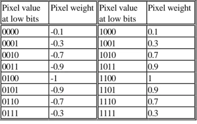
(2) Pixel value at low bits 0000 0001 0010 0011 0100 0101 0110 0111. Pixel weight Pixel value at low bits -0.1 1000 -0.3 1001 -0.7 1010 -0.9 1011 -1 1100 -0.9 1101 -0.7 1110 -0.3 1111. Pixel weight 0.1 0.3 0.7 0.9 1 0.9 0.7 0.3. Table 1: The weighting table corresponds to higher probability. For example, a pixel value of 11000000 with four LSBs of 0000 is mapped to the weighting of –0.1 while another pixel value 11000001 with the same four MSBs but with different four LSBs of 0001 is mapped to the weighting of -0.3. The difference of the magnitudes of these two pixels is only 1, which means that it is very likely that the first pixel value of 11000000 is changed to the second pixel value of 11000001 under some kind of processing. The idea of embedding watermark information in this paper is to gradually change the pixel value until the corresponding weighting achieves a predefined threshold value. The process of changing the pixel values is called finetune process whose objective is to have as small pixel magnitude change as possible while still maintaining the robustness of the watermarking scheme.. 2.1 Basic Watermark embedding scheme In order to increase the robustness, we consider adding one watermark bit for a group of pixels, say four pixels for each watermark bit as will be shown shortly. Assume that the size of the original gray-level image is N×N and the watermark bits are from a binary image of M × M with pixel values ∈{1, −1} . The watermark embedding procedure is listed below and illustrated in Fig. 1. E-(1): Divide the original image into four regions (A,B, C, D) of the same size. E-(2): Partition each region into blocks of size 8 × 8 . E-(3): Calculate the variance of all the 8 × 8 blocks and select the M2 /64 blocks with the largest variances for watermark embedding. Number the blocks according to the order of their variance. If we want to reduce the computation complexity, this step of block variance calculation can be skipped by selecting randomly M2 /64 blocks in each region instead. However, embedding watermark bits into image blocks of large variance will reduce the influence on image quality since human visual system is less sensitive to the pixel value changes of image blocks with large variance. E-(4): Denote the pixel value at the j-th position of the i-th 8 × 8 block in region A, B, C, D as Ai,j ,Bi,j ,C i,j ,Di,j respectively where 1 ≤ i ≤ M 2 / 64 , 1 ≤ j ≤ 64 .. E-(5): Map a group of four pixels Ai,j ,Bi,j ,C i,j ,Di,j into their corresponding weightings using Tab. 1. ′ ′ ′ ′ Ai, j , Bi, j , Ci, j , Di, j E-(6): Based on the k-th binary watermark bit Wk ∈ {1, −1} , calculate if the following inequality (1) is satisfied (1) ( Ai′, j ,+Bi′, j + C′i, j ,+Di′, j ) ×Wk ≥ T1 where T1 is the prescribed threshold that is a function of the number of pixels in each group. Note that the selection of this threshold affects the image quality and the robustness performance of the watermarking scheme. In our experiment, T1 is set to be 2.5 for group size of 4. If inequality (1) is satisfied, the watermark bit Wk has been already added to the group of four pixels Ai,j ,Bi,j ,C i,j ,Di,j. Then continue the embedding steps E-(5) and E-(6) for another group of four pixels. If not, proceed to the following fine-tune process. E-(7): Based on the sign of the watermark bit Wk , change the magnitudes of Ai,j ,Bi,j ,C i,j ,Di,j to their neighboring pixels ~Ai, j , B~i , j , C~i, j , D~i, j with the weightings closer to the value Wk . Then continue steps E-(5) and E-(6). The following exemplifies our watermark embedding procedure. Assume that we want to add a watermark bit Wk = -1 into the group of four pixels with values Ai , j = 10111111 , Bi, j = 11000000 , C i, j = 00100111, Di , j = 00110011. According to the pixel weighing in Tab. 1, we have the corresponding weightings A′i, j = 0 .3, B′i, j = −0 .1, C′i, j = −0 .3,. D′i, j = −0 .9. The sum of the above four weightings is –1 and inequality (1) is not satisfied. Thus, we change the four pixels to their neighboring pixels with weightings closer to Wk = -1, i.e., ~ Ai , j = Ai, j + 1 = 11000000 , ~ Ci, j = Ci, j − 1 = 00100110 ,. ~ Bi, j = Bi, j + 1 = 11000001 , ~ Di, j = Di, j + 1 = 00110100. The corresponding weightings of the above fine-tuned pixels are ~ Ai′, j = − 0. 1,. ~ Bi′, j = −0 .3,. ~ Ci′, j = −0 .7 ,. ~ D i′, j = −1. The sum of the above four weighting values does not satisfy inequality (1) either, and thus we continue another ~ ~ ~ ~ fine-tune process by replacing A i , j , B i, j , Ci , j , Di , j with their neighboring pixels..

(3) A B. calculate variance of each block. C D Original Image. select M 2 / 64 blocks with largest variance. partition into four regions and divide each region into 8 x 8 blocks. M. M. W watermark image. 8. (1) satisfied?. no. reference pixel?. 8. 1. 2. 3. 4. 5. 9. 10. 11 2. 12. 13. M yes. yes no. 1 9 fine-tune 8. all pixels processed?. 2. 6. 7. 8. •••. / 64 blocks at one region of the original image 8 •• 8 • •• •. • • •. next pixel no. 64. ye s. one 8*8 pixel block. finish. Fig. 1: The watermark embedding procedure.. ~ Aî , j = Ai, j + 1 = 11000001 , ~ Cî, j = Ci , j − 1 = 00100101 ,. ~ Bî , j = Bi , j + 1 = 11000010 , ~ Dî , j = Di, j = 00110100. The corresponding weightings are Aî′, j = − 0. 3,. Bî′, j = −0. 7,. Cî′, j = −0 .9,. Dˆ′i, j = −1. in other blocks have small changes. We can use the reference pixels to calculate the degree of changes under a specific signal processing. In this case, each 8 x 8 block should be assigned a factor indicating reliability (fidelity) of this block. Using the same mapping table of Tab. 1, we obtain the weightings of the 16 reference pixels in the 8 x 8 block of Fig. 2 and denote them as Rk′ , k = 1,2, Λ ,16 . Let. The above weighting satisfies inequality (1) and thus the fine-tune process terminates.. P=. 16. ∑ Rk′ (−1) k. (2). k =1. 2.2 Improved Watermark Method with Reference Pixels We can increase the robustness and security of the above watermarking method by dividing the pixels in each 8 x 8 block into two categories: reference pixels and embedding pixels. For example, the pixels in the 8 x 8 block of Fig. 2 are divided into 48 embedding pixels and 16 reference pixels where the reference pixels are located in three diagonals. The watermark information is added into the embedding pixels while the reference pixels are used to detect the reliability of this 8 x 8 block. Indeed, after some geometric distortion, pixel values in some blocks might be changed significantly while pixel values. The same fine-tune method as in Sec. 2.1 is used for the 16 reference pixels so that inequality P ≥ T2 is satisfied. The threshold valueT2, affecting the reliability, is selected to be 10 in our experiment. The watermark embedding method for other embedding pixels is the same as discussed before in Sec. 2.1. Later in Sec. 4, we will see that such a watermark embedding method with reference pixels has better performance. Since only 48, instead of 64, watermark bits are added for each 8 x 8 block, the number of blocks selected for watermark embedding in each region should be M2 /48.

(4) If ( Pi (a ) Ai′, j + Pi (b ) B i′, j + Pi (c )C i′′, j + Pi (d ) Di′, j ) ≥ 0 then Wk′ = 1; else Wk′ = 0. 8 1. 2 3. 4 5. 8. Reference Pixel 6. 7 9. 8. Embedding Pixel. 10 11. 14 15. Pi(a), P i(b) , P i(c) ,P i(d) are respectively the reliability metrics of the four i-th 8 × 8 blocks where the four pixels with weightings A ′i′, j , Bi′′, j , C i′′, j , D i′′, j are located. The four reliability metrics, calculated using Eqn. (2), are used as the scaling factors to determine the confidence of the four weightings A ′i′, j , Bi′′, j , C i′′, j , D i′′, j if the pixel values in. 12 13. (4). 16. Fig. 2: Embedding pixels and reference pixels in an 8 x 8 block. instead of M2 /64. Although the positions of the reference pixels in each block are fixed in Fig. 2, it is possible to arbitrarily select the positions of these reference pixels in order to increase the security of the watermark method. For example, the location of the reference pixels may come from a pseudo random sequence generator.. 3. WATERMARK EXTRACTION AND DETECTION The watermark decoding process contains two stages. The first stage is to extract watermark sequence from the received image, which might undergo any kind of signal processing or attack. The second stage is to detect whether the received image contains the desired watermark based on the extracted sequence and the original watermark sequence. We will discuss these two stages in the following.. some part of the image encounter significant changes due to geometric distortion, common signal processing, or other subterfuge attacks. Recall that in the watermark embedding process mentioned in Sec. 2, the reliability metric of an 8 × 8 block is fine-tuned to be greater than or equal to a threshold value T2 (T2 = 10 in our experiments). Thus, if any one of Pi(a), P (b) , P i(c) ,P i(d) is greater than 10, we limit it to 10 while if some i of Pi(a), P i(b) , P i(c) ,P i(d) are smaller than 1 (due to the serious attacks), we assign the value of 1 for them. If the four values are in between, i.e., 8 ×8 1 ≦ Pi(a), P i(b) , P i(c) ,P i(d) ≦ 10, their values are used as the scaling factors for inequality (4) during the watermark extraction. Inequality (3) is in fact a special case when the scaling factors Pi(a), P i(b) , P i(c) ,P i(d) of the i-th block are all one. Shortly, we will see that the watermark scheme with referencepoint has better performance.. 3.2 Watermark Detection After extracting watermark bit sequence the normalized correlation of random sequence. Wk′ , we calculate. Wk′ with the original pseudo. Wk in order to determine whether the. extracted sequence is the correct watermark bit sequence. The normalized correlation of the two sequences are defined as. 3.1 Extraction of Watermark Sequence Our proposed watermark extraction method does not require the access of the original image data. The extraction process is quite simple. Assuming that Ai′, j , Bi′′, j , C′i′, j , Di′′, j are the. Corr(W , W ′) =. corresponding weighting values of the four pixels from the same position of the four regions in the received image, we can determine the corresponding watermark bit Wk′ as. where IP( A , B ) is the inner product o f two sequences. follows:. larger than a threshold value, i.e.,. If ( Ai′′, j + Bi′′, j + Ci′, j + Di′′, j ) ≥ 0, then Wk′ = 1 else Wk′ = 0. (3). In other words, the sign of the summation of the corresponding four weighting values determines the embedded watermark bit. If the reference-pixel method proposed in Sec. 2 is adopted to enhance the robustness, the above watermark extraction is modified as follows:. IP(W , W ′) IP (W , W ) × IP(W ′, W ′). Ak , Bk . If the normalized correlation of the two sequences is Corr(W ,W ′) ≥ T3. (5). the extracted watermark sequence is determined to be the same as the original embedded sequence. The selection of the threshold value T3 affects the false detection rate or false pass rate. In the following, we give a systematic method to choose this threshold value..

(5) (a) original Lena. (b) watermark Lena-I. (c) watermark Lena-II. (PSNR= 44.7). (d) original baboon. (PSNR= 43.4). (e) watermarked baboon-I (PSNR=46.1). (f) watermarked baboon-II (PSNR= 46). Fig. 3: The original images of Lena (a) and baboon (d) and those after embedding watermark bits using our proposed methods without (b)(e) and with (c)(f) reference pixels.. 4. EXPERIMENT RESULTS. According to the central limit theorem, the normalized The test images we use in this experiment are Lena and correlation X = Corr (W , W ′) of the extracted watermark baboon of size 256 x 256 with gray levels of 8 bits for each sequence and all the other pseudo random sequences can be pixel. The embedded binary watermark bit sequence with approximated as a random variable with Gaussian distribution. length of 32*32 is the 200th sequence among the 1000 pseudoX − µ with sample mean µ and sample randomly generated sequences. For convenience, our Thus, Z = proposed watermark methods without and with reference σ pixels are noted respectively as method-I and method-II. We variance σ 2 is a normalized Gaussian distribution Q(z) first examine the invisibility of our proposed watermark with zero mean and standard deviation of one methods by calculating the peak-signal-to-noise-ratio (PSNR) for the two watermark images. It is almost imperceptible as can 2 x be observed Fig. 3. z − 1 2 Next, we compare the performance of our proposed Q( z ) = e dx watermark methods with other approaches under a variety of − ∞ 2π signal processing or attacks as shown in Tab. 2 for Lena image. . Let the threshold is selected as T3 = ασ , the probability Two types of geometric distortion (cropping and dilation), two of false watermark detection is types of common signal processing (JPEG and equalization) and the subterfuge attack of the last three LSB bits are considered. The values in Tab. 2 are the normalized correlation Pr ob{ X > T3 } ≤ Q(α ) . (6) of the extracted watermark sequence with the original sequence. Based on the analysis in Sec. 3, the threshold of the In other words, the probability of detecting the watermark correlation is set to be 0.1 with the probability of false sequence for non-watermark images is less than Q (α) . Thus, detection smaller than 10 −4 . In other words, watermark we can select the threshold value T2 depending on this sequences with correlation smaller than 0.1 is determined to be probability which might vary from applications to applications. undetectable since they are not significantly larger than. ∫.

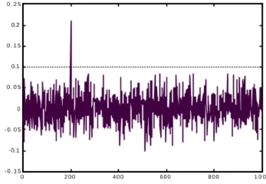
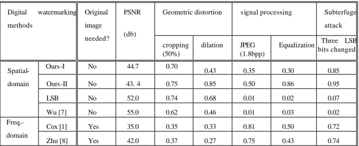
(6) 0.25. (6) Our proposed spatial-domain watermarking methods have better overall performance and they do not need the original image during watermark extraction. Furthermore, the methods are simple and easy to realize using either hardware or software.. 0.2. 0.15. Corr. 0.1. 0.05. 0. -0.05. -0.1. -0.15 0. 200. 400. 600. 800. 1000. Fig. 4: The normalized correlation of the extracted watermark sequence with all the 1000 pseudo random sequences (our proposed method under JPEG processing). the correlation with other no-watermark sequence. Since the embedded watermark bits are from the 200th sequence, the correlation of the extracted watermark sequences with the 200th sequence should be much larger than the correlation with all the other 999 random sequences, as indicated in Fig. 4. From Tab. 2, we have the following observations: (1) Most of the digital watermark methods have high PSNR (greater than 40) except for the method proposed by Cox [1]. As can be seen from Fig. 3, images with PSNR greater than 40 are almost indistinguishable with the original images. (2) Most of the frequency-domain methods require the original image during watermark extraction. Thus, their applications are limited and a large memory space is needed to store the original images before watermark extraction. (3) Compared with frequency-domain approaches, the spatialdomain watermarking methods usually have better performance under geometric distortion but have poor performance under common signal processing and subterfuge attacks. For example, the normalized correlation values for the listed two frequency-domain methods under 50% cropping are around 0.3-0.4 compared to those of 0.7-0.8 using spatial-domain methods. On the other hand, the correlation values of the frequencydomain methods under JPEG processing with 1.8 bit-perpixel (bpp) are 0.7-0.8, much higher than those using spatial-domain methods. (4) Most spatial-domain methods are vulnerable to common signal processing such as JPEG and filtering. For example, the correlation values using the LSB method and the method proposed in [8] are smaller than the threshold value of 0.1. Hence, the embedded watermark information is lost. However, our proposed methods are robust to this kind of signal processing or filtering. (5) Our proposed method with reference pixels have better robustness performance than without using reference points at the cost of slightly lower PSNR (but still greater than 40). For example, the correlation value is increased from 0.43 to 0.85 for the watermark image with dilation.. We also tested three benchmark images (Lena, baboon and F-16) using our proposed watermark methods with and with reference pixels. The experimental results are shown in Tab. 3 where ours-I is the method without reference pixels while oursII is that with reference pixels. The watermark embedding method with reference pixels is in general has better performance.. 5. CONCLUSIONS We proposed two spatial-domain watermarking methods based on a pixel-weighting table and the fine-tune process. The methods, although simple, have better robustness performance compared to other spatial-domain or frequencydomain methods. Furthermore, our methods do not require the original image during watermark extraction, make them favorable for most watermark applications.. References [1] I. J. Cox, J. Kilian, T. Leighton and T. Shamoon, ”Secure Spread Spectrum Watermarking for Multimedia”, IEEE Trans. On Image Processing, Vol. 6, No12, pp.1673-1687, Dec. 1997. [2] M. D. Swanson, M. Kobayashi, and A. H. Tewfik, “Multimedia Data-Embedding and Watermarking Technologies”, Proc. of IEEE, Vol. 86, No.6, pp.1064-1087, June 1998. [3] C.-T. Hsu and J.-L. Wu, “Hidden Digital Watermark in Image”, IEEE Transactions on Image Processing, Volume: 8 1, pp 58 –68, Jan. 1999. [4] W. Tang and Y. Aoki, “A DCT-based Coding of Images in Watermarking”, Information, Communications and Signal Processing., Proc. ICICS, Volume: 1 , pp 510 -512, 1997. [5] I. J. Cox, Jean-Paul M. G. Linnartz, “Some General Methods for Tampering with Watermarks”, , IEEE Journal on Selected Areas in Communications, Volume: 16 4 , pp 587 -593 , May 1998. [6] R. B. Wolfgang and E. J. Delp, “A Watermark for Digital Image”, Proc. IEEE Intl. Conf. on Image Processing, Volume: 3 ,pp 219 -222, 1996 . [7] M. Wu, and B. Liu, “Watermarking for image authentication”, Proc IEEE Intl. Conf. on Image Processing, vol. 2, pp. 437-441, 1998. [8] W. Zhu, and Z. Xiong and Y. Q. Zhang, “Multi-resolution watermarking for images and video”, IEEE Transactions on Circuits and Systems for Video Technology, vol. 9, no. 4, pp. 545-550, Jun. 1999..

(7) Digital. watermarking. methods. Original. PSNR. Geometric distortion. signal processing. Subterfuge. image needed?. attack (db) cropping (50%). Spatial-. Ours-I. No. 44.7. 0.70. Ours-II. No. 43. 4. LSB. No. Wu [7]. domain. Freq.domain. dilation. JPEG (1.8bpp). Equalization. Three LSB bits changed. 0.43. 0.35. 0.30. 0.85. 0.75. 0.85. 0.50. 0.86. 0.95. 52.0. 0.74. 0.68. 0.01. 0.02. 0.07. No. 55.0. 0.62. 0.46. 0.01. 0.03. 0.02. Cox [1]. Yes. 35.0. 0.35. 0.33. 0.81. 0.50. 0.72. Zhu [8]. Yes. 42.0. 0.37. 0.27. 0.75. 0.43. 0.74. Tab. 2: Comparison of robustness of different watermarking methods under a wide variety of signal processing.. Three test images. Lena. baboon. F16. PSNR. Geometric distortion. signal processing. cropping. dilation. JPEG. Equalization. Ours-I. 44.7. 0.70. 0.43. 0.35. 0.30. Ours-II. 43.4. 0.75. 0.85. 0.5. 0.86. Ours-I. 46.1. 0.78. 0.43. 0.20. 0.10. Ours-II. 46. 0.78. 0.74. 0.10. 0.10. Ours-I. 44.8. 0.86. 0.21. 0.32. 0.18. Ours-II. 43. 0.69. 0.94. 0.49. 0.90. Tab. 3: Performance comparison of our proposed watermark methods for different benchmark images..

(8)