Low-lying exciton states in a type-II broken-gap quantum well structure: A variation-basis-set approach

CHINESE JOURNAL OF PHYSICS’ VOL. 35, NO. 2 APRIL 1997

Low-Lying Exciton States in a Type-II Broken-Gap Quantum Well Structure: A Variation-Basis-Set Approach

C. S. Chu and K. D. Chu

Department of Electrophysics, National Chiao Tung University, Hsinchu, Taiwan 300, R.O.C.

(November 19, 1996)

The exciton binding energy and the low-lying exciton states in a type-II broken-gap quantum well structure are studied. The conduction electron and the hole that form the exciton are spatially separated and are each confined by a quantum well. A variation-basis-set approach is proposed in which a set of variation basis set wavefunctions are constructed from the eigenstates of a variation Hamiltonian. The calculation of the exciton states can be carried out systematically and the accuracy of the state energies can be estimated. Numerical examples are presented, showing the rapid convergence of the excitonic levels with respect to the size of the variation basis set in and beyond the small well width regime. The effective binding energies for the states are found to increase with the decreasing of the well width. The low-lying exciton states in and beyond the small well width regime are presented.

PACS. 71.35.-y - Excitons and related phenomena. PACS. 31.15.Pf - Variational techniques.

PACS. 73.20.-r - Surface and interface electron states.

Excitons in semiconductor heterostructures have been of continued interest, both theoretical and experimental [l-9], in the past two decades. The reasons are firstly, that the excitons can affect significantly the optical properties of the structures. Secondly, that the exciton gas, being generated in semiconductor quantum well structures, is a system favorable for the search of an excitonic phase [g-11]. However, in a type-1 heterostructures, which are the most studied semiconductor structures, the excitons are formed from electrons and holes confined in the same quantum well and thus the exciton state is susceptible to the recombination between the two types of charge carriers. This recombination problem is expected to be removed in a type-II broken-gap quantum well structure [1,2].

A type-II broken-gap quantum well structure involves, apart from the wide band gap barrier material, two semiconductors of which the respective band gaps do not overlap in energy [12,13]. The valence band edge of one of the semiconductors lies in energy above the conduction band edge of the other semiconductors, resulting in transferring of electrons from the former to the latter semiconductor, when the quantum well widths are not too small. This spatial separation of electrons and holes allows for the formation of much stable excitons. The recombination between the electrons and the holes can be further suppressed by inserting a separating barrier, formed from a wide band gap material, in between the 164 @ 1996 THE PHYSICAL SOCIETY OF THE REPUBLIC OF CHINA

VOL. 35 C.S.CHUAND K.D.CHU 165

two semiconductors. The confinement on the electrons and the holes can be imposed from barriers fabricated at both ends of the structure. The exciton binding energy is increased by decreasing the well width but is decreased by increasing the spatial separation of the electrons and the holes.

The exciton binding energy in such type-II broken-gap quantum well structures, but with small well widths (L << a*), has been studied by Bastard et al. [l], Zhu et al. [3], and Xia et al. [6], using various versions of variational wavefunctions in their calculations. Here a* is the effective Bohr radius. Alternatively, an expansion method has been proposed [6] in which the subband wave functions for the electron and the hole are used as the basis. This expansion method leads to a group of coupled differential equations, which has to be solved numerically. Though general in its approach, the expansion method is too involved numerically. On the other hand, the variational wavefunction approach is simple in its calculation, but gives only the ground exciton state. In all these methods, however, the forms of the wavefunctions have been chosen such that they are more appropriate for narrow well width cases. Thus we propose, in this work, a variation-basis-set approach which appropriateness covers larger well widths (0 < L N a*), while it is efficient numerically. Furthermore, the method can be used to obtain the excited states.

The variation-basis-set approach is an extension of a perturbative-variational method proposed by Mei and Lee [14,15], who used a variation hamiltonian, instead of a variation wavefunction, in their study of the impurity states in anisotropic crystals. The difference between the actual and the variation hamiltonian was treated perturbatively. By imposing a rapid convergence condition on the first order energy term in the perturbation expansion, the value for the variation parameter as well as the ground state energy were determined. This method is very general and has been applied to the finding of the exciton binding energy in type-1 quantum well systems [16-181. The effectiveness of the method hinges on the choice of the variation hamiltonian, which has to be tractable yet retaining the essential physics of the actual hamiltonian. In this work, we propose to make a better use of the basis set of wavefunctions that are constructed from a variation hamiltonian. We first introduce a variation hamiltonian for the type-II broken-gap quantum well systems and then construct a basis set of wavefunctions from the eigenstates of the hamiltonian. The basis set of wavefunctions are, by construction, orthogonal and variational, and is used to diagonalize the actual hamiltonian. Finally, the variation parameters are determined from minimizing the ground state energy.

In our calculation, the dielectric constant 6 is taken to be a constant throughout the type-II broken-gap quantum well. For the barrier layer, the band gap is assumed wide enough, encloses not only the band gaps of both the electron and the hole layer materials, but allows us to approximate it as an infinite potential barrier. The electron mass rn: and the hole mass ml are the effective masses of the respective materials, with rn; taken to be that of the heavy hole. The above assumptions are reasonable for a qualitative study and for a typical type-II broken-gap system such as the GaSb-AlSb-InAs quantum well structure [l,S]. The purposes of this paper are: to present model calculations for the well width dependence of the low-lying exciton states, and to present an approach which can be easily extended to more quantitative studies in the future.

166 LOW-LYING EXCITON.STATES IN A TYPE-II BROKEN-GAP _{VOL. 35}

FL2

HE--V,2,--2m;

fi2 772 _ e2

2rni rh _{fir, - fhl} + V&e) + V/&J?

where V,, Vh are the confining potentials of the quantum wells for the electron and the hole, respectively. As have been mentioned above, we assume a perfect confinement for both of the charges [6] so that the confining potentials V,, Vh are infinite square well potentials. For simplicity, we consider the symmetry case where the two well widths L are the same. The coordinates for the electron z, and the hole .zh are measured from the interface between the separating barrier and the respective well. Without loss of generality, we shall drop, from Eq. (l), the kinetic energy due to the motion of the center of mass parallel to the interface. The hamiltonian is then given by

H=

-fW;-&$-

e h dp2 + (Ze + zh + w)2 +x(Ze) f vh(zh)

,

(2)

where y = mz/m;l, and ,O = ml/p. Here w is the width of the separating barrier, p =

mEml/(rnz + m;E) is the reduced mass, and p’ = (r, - rh)ll is the relative displacement parallel to the interface. In obtaining Eq. (a), we have chosen the effective Bohr radius cz* = h”c/(mze”), and the effective Rydberg R’ = e2/(2eu*).

We introduce a variation Hamiltonian 8

I;T = H, + H/, + flFI,, ₍₃₎ where and

“, +

KCze)7

$

(4)

(5)

In the variation hamiltonian a, the perpendicular motion of the electron and the hole are given by H, and Hh, respectively, which have incorporated the effect of the hole (electron) on the electron (hole) in H, (Hh) through a coulombic term characterized by a positive variation parameter a (b). We point out that this choice of the variation hamil-tonians H, and Hh has the nice features that the confining potentials dominate when L

is small and the term dominates when L is large. Thus H, and Hh should be appropriate from the small L (L < a*) to the large L (L > a*) regime. The eigenstates and eigenvalues for these two hamiltonians, with the dependence on the variation parameters not explicitly shown, are given by

VOL. 35 C. S.CHU AND K. D. CHU 167

(7)

and are solved numerically by a Runge-Kutta procedure.

The hamiltonian H, is a two-dimensional hydrogenic hamiltonian with an effective electron charge -e*e, where -e is the charge of a free electron. The eigenstates I$I~,~,~) are given by

(p’i$~~,~,~) = A eim4

film’

w h e r e @ = e-p//3, m = 0,&l, 4~2 .., k = 0,1,2.., and nz = k + jrnl + f. Here A is the normalization constant, F(cY,&,u) is the Kummer function, m is the azimuthal quantum number, and EPVrn,k = -e*2/(/3ni) is the corresponding energy eigenvalue.

The choice of the variation hamiltonian a seems to have the two dimensional (2D) motion decoupled from the one dimensional (1D) motion. This decoupling is roughly the case for L < a*, as have been considered in previous variational studies [l, 3,5,6]. But in the case of not-so-narrow well widths, a better scheme has to include the coupling between the 2D and the 1D motions. This coupling feature is taken into account here by a heuristic relation that determines the value of e’. An electric-field-balancing argument [19] is used to obtain the relation

(10)

w h e r e Z,R = .z,,-~ t a t w. Here G,,,, is the position at which I(z,/$J,,~)~~ is at its maximum, and peff is determined from the maximum of I(p($~~,~,n)l~p. A straightforward calculation gives peff = p (2]mj t 1)2/(4e*). T he d pe endence of e* on 20, m, and a provides the coupling between the perpendicular and the parallel motions of the electron and the hole. This choice of e* is found to greatly enhance the efficiency of the exciton states calculation.

The eigenstates for I? is denoted by

where N represents the set i,j, and k. The azimuthal quantum number m is a good quantum number for both fi and H. The exciton ground state is the lowest energy eigenstate of H, with m = 0. The excited states of the exciton are the higher energy eigenstates of H with m = 0, and all the eigenstates of H with m # 0. Traditional variation method can provide an approximation to the lowest energy eigenvalue for each m. Here we proceed to calculate the other excited states systematically.

In our approach, for a fix m, the wavefunctions Is?) form a variation basis set which, by construction, is orthogonal and variational. Using these wavefunctions, we obtain the matrix elements H,yi:,, = (@jJHj$~,), which expression is given by

LOW-LYING EXCITON STATES IN A TYPE-II BROKEN-GAP VOL. 35

In principle, when the entire basis set of wavefunctions are used, the exciton energy levels

EE should not depend on the variation parameters. But in practice, when only a finite number of wavefunctions from the basis set are used, the energy levels would depend on the variation parameters. Therefore, we fix the values of a, and b by the conditions

aHG =

da

’

(13)

The low-lying exciton levels EF, where N = 0, 1,2,. . . , with N = 0 corresponds to the lowest levels of the series, are determined from the condition

det]HgNj - E 6~ppI = 0. ₍₁₅₎

In our numerical examples, we take the type-II broken-gap systems to be the GaSb-AlSb-InAs systems where the valence band edge of GaSb is higher in energy than the conduction band edge of InAs, with AC = E,(GaSb)- E,(InAs) = 0.175eV [S]. In addition, as a result of the quantum well confinement, an effective indirect energy gap EG = -AC f

E,,o + Eh,O - EB can be used to indicate whether the electron and the hole favor spatial

separation [6]. Here EB = E,,o + Eh,O - Eo is the exciton binding energy. The indirect energy gap EG can be tuned from positive to negative by increasing the well width L. The electron and the hole prefer spatial separation only when EG is negative. This is the region considered in our numerical examples.

For the other physical parameters, we have rnz = O.O23m,, m;l. = 0.4m,, and 6 = 14.7. Thus a* = 338 A, and R* = 1.45meV. In our calculation, for a given m, we h a v e chosen up to six wavefunctions from the basis IQ?;). These wavefunctions involve the states

~~e,o)~‘+h,o)~~~,m,k 7) where only the lowest energy states from H, and H,I, are included. We have attempted to include, in the basis set, higher energy states from H, and Hh, but the effect on the low-lying exciton states is found to be very small.

In our numerical results, we plot the effective binding energies E$ = E,,o+ Eh,O - E$, instead of the energy levels EF, for the exciton states. Had we included the complete basis set of fi, the effective binding energies E$’ would have been exactly determined. But, in practice, we can only include a finite basis set. Hence the effective binding energies, denoted

VOL. 35 C. S. CHU AND K. D. CHU 169

by E,“(M), will depend on the size A4 of the basis set. The effectiveness of our approach can be tested by tracing how rapid k,“(M) converges to J!!?; as M increases, as we will present in the following.

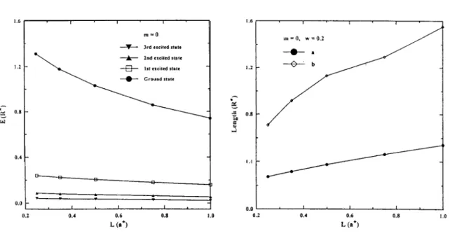
The results for the m = 0 case are shown in Figs. (l)-(3). In Fig. 1, the m = 0 exciton energy levels, represented by their corresponding effective binding energies, are plotted as a function of the well width L. The separating barrier width w = 0.2 and the range of L is up to a”. In all four of the energy levels shown, their effective binding energies increase as L decreases. The ground state binding energy @, which varies over 0.5 R’ in Fig. 1, is most sensitive to L. The values of the variation parameters a and b depend on L and, as shown in Fig. 2, the dependence on L is quite smooth which shows the numerical stability of the results.

Since the maximum basis set size used in this calculation is M = 6, the effective binding energies shown in Fig. 1 are actually E;(S). H owever, these values are very close to the exact values, because the uncertainties in the &,$(6) values is found to be small. Both the uncertainties in E&(6), and the rapid convergence of the E;(M) values with respect to M are presented in Fig. 3. In Fig. 3, the deviation A$&(M) = E;(M) - E&(6) is plotted against L, for M = 1,4, and 5. The E;(l) is defined as (~~IHj\k~). The convergence is quite rapid and the estimated uncertainties of the respective levels can be read off from the

1.6

I.?.

0.4

FIG. 1. Four lowest m = 0 exciton levels ver-sus well width L. The barrier width w = 0.2. The levels are given in terms of the effective binding energy ki, with N = 0 corresponds to that of the ground exciton state.

FIG. 2. The variation parameters a, b versus well width L for m = 0, and w = 0.2.

-1 7 0 LOW-LYING EXCITON STATES IN A TYPE-II BROKEN-GAP VOL. 35 0.002 - ~,

1

t

FIG. 3. The convergence of the four lowest m = 0 exciton levels E;(M) with respect to the size M of the variation basis set is shown for various L . The barrier width w = 0.2. The curves indicated by X, 0, and l correspond to the deviation of the energies E;(l), E&(4),

and E;(5), respectively, from the energy g:(S). Graphs in (a) are for the ground state (N = 0), while graphs in (b), (c), and (d) are for the excited states, with N = 1,2, and 3, respectively. The convergence is quite rapid and the estimated uncertainties of the respective levels can be read off from the curves indicated by 0.

values of A,!?N(~). From Fig. 1 and Fig. 3, it is found that the relative uncertainties in Es are less than 0.02%, 0.5%, 2%, and 3%, for N = O,l, 2, and 3, respectively. In addition, the binding energy in the small L (L < a*) regime compares favorably with previous variational results [1,3].

VOL. 35 C.S.CHU AND K. D.CHU 171

FIG. 4. Four lowest m = 1 exciton levels ver-sus well width L. The barrier width w = 0.2. The levels are given in terms of the effective binding energy

0.0 - .

-2.0

1

0.2 0.4 0.6 0.8 1.0

L (a’)

FIG. 5. The variation parameters a, 6 versus well width L for m = 1, and w = 0.2.

The results for the m = 1 case are shown in Figs. (4)-(6). In Fig. 4, the four lowest m = 1 exciton energy levels, represented by their effective binding energies l.?;, are plotted as a function of L. Again, all the effective binding energies increase as L decreases. The N = 0 state, also called the 2p state, [20] h as the largest effective binding energy of the series. IIowever, this is not the ground exciton state. The values of the variation parameters a and b are shown in Fig. 5, which dependence on L is quite linear. In Fig. 6, the deviation A,!?h(M) = E,$(M) - E,$(6) is plotted against L, for M = 1,4, and 5. The Ek(l) is defined as (Gh]H]*,$). T he convergence is quite rapid and the estimated uncertainties are given by the values of A&h(5). From Figs. (4) and (6), the relative uncertainties in ,??A are found to be less than 0.05%, 0.5%, 1.5%, and 2%, respectively. These results show the effectiveness of our approach.

This variation-basis-set approach can be extended quite straight-forwardly to the case beyond perfect confinement, and also to the case when an external electric or magnetic field is applied parallel to the growth direction.

In conclusion, we have proposed a variation-basis-set approach to calculate the low-lying exciton states of a type-II broken-gap quantum well structure. The approach can be applied to a large range of well width L and the effectiveness is demonstrated.

172 LOW-LYING EXCITON,STATES IN A TYPE-II BROKEN-GAP VOL. 35

FIG. 6.

0.2 0.4 0.6 0.8 1.0 I. (37

The convergence of the four lowest m = 1 exciton levels EL(M) with respect to the size M of the variation basis set is shown for various L. The barrier width w = 0.2. The curves indicated by x, 0, and l correspond to the deviation of the energies E;(l), Eh(4),

and ,!?,$(5), respectively, from the energy E;(6). Graph s in (a) are for the lowest level (N = 0), while graphs in (b), (c), and (d) are for the excited states, with N = 1,2, and 3, respectively. Note that the two curves indicated by 0, and l in (a) are almost on top of one another. The convergence is quite rapid, and the estimated uncertainties of the respective levels can be read off from the curves indicated by 0.

A c k n o w l e d g m e n t

This work was partially supported by the National Science Council of the Republic of China through Contract No. NSC83-0208-M-009-060.

VOL. 35 C. S. CHU AND K. D. CHU 173

References

[ 1 ] G. Bastard, E. E. Mendez, L. L. Chang, and L. Esaki, Phys. Rev. B26, 1974 (1982). [ 2 ] S. Datta, M. R. Melloch, and R.L. Gunshor, Phys. Rev. B32, 2697 (1985).

[ 31 X. Zhu, J. J. Qumn, and G. Gumbs, Solid State Commun. 75, 595 (1990). [ 41 G. E. W. B suer, Solid State Commun. 78, 163 (1991).

[ 5 ] S. V. Branis, and K. K. Bajaj, Phys. Rev. B45, 6271 (1992). [ 6 ] X. Xia, X. M. Ch en, and J. J. Quinn, Phys. Rev. B46, 7212 (1992).

[ 7 ] R. C. Miller, A. C. Gossard, W. T. Tsang, and 0. Munteanu, Phys. Rev. B25, 3871 (1982). [ 8 ] J. E. Golub, P. F. Liao, D. J. Eilenberger, J. P. Harbison, and L. T. Florez, Solid State

Commun. 72, 735 (1989).

[ 9 ] J. P. Cheng, J. Kono, B. D. McCombe, I. Lo, W. C. Mitchel, and C. E. Stutz, Phys. Rev. Lett. 74, 450 (1995).

[lo] B. Bucher, P. Steiner, and P. Wachter, Phys. Rev. Lett. 67, 2717 (1991). [ll] Y. Kuramoto, and C. Horie, Solid State Commun. 25, 713 (1978).

[12] L. Esaki, in Novel Materials and Techniques zn Condensed Matter, eds. G. W. Crabtree and P. Vashishta (Elsevier, Amsterdam, 1982), p.1.

[13] E. T. Yu, J. 0. McCaldin, and T. C. McGill, Solid State Physics 46, (1992) p.4. [14] W. N. M er and Y. C. Lee, Physica 98B, 21 (1979).‘,

[15] Y. C. Lee, W. N. Mei, and K. C. Liu, J. Phys. C15, L469 (1982). [16] T. F. Jiang, Solid State Commun. 50, 589 (1984).

[17] U. Ekenberg, and M. Altarelli, Phys. Rev. B35, 7585 (1987). [18] D. S. Chuu, and Y. T. Shih, Phys. Rev. B44, 8054 (1991).

[19] From the wavefunctions ]$J~,IJ) and ]$~~,~,c), we can define the typical distances peg and 2,~ between the electron and the hole, along and perpendicular to the 2D layer, respectively. Along the 2D direction, the electric field between the two charges is given by ep,R/(pzff + z&)3/2, The electric-field-balancing argument requires this electric field to be reproduced by the electric field of the effective charge in H,, given by e*e/p&. Thus we obtain the heuristic relation in Eq. (10). That this heuristic relation has incorporated the coupling between the 2D and the 1D motions is made clear in the above discussion. Furthermore, it turns out that the heuristic relation greatly improves the efficiency of our calculation. This assures us that the coupling feature has been appropriately included in this heuristic relation.

[20] A. H. M Dac onald, and D. S. Ritchie, Phys. Rev. B33, 8336 (1986).