ESTIMATION OF MULTIPLE SINUSOIDAL FREQUENCIES USING TRUNCATED LEAST-SQUARES METHODS

990 IEEE TRANSACTIONS ON SIGNAL PROCESSING, VOL. 41, NO. 2, FEBRUARY 1993 and then p(S) = 1 . Now suppose that p ( S ) 2 p

>

1 and that the

boundary values of Gp- I are infinite. From ( 1 2 ) a boundary value of Gp can be finite only if

/BPI

= 1, then from (1 1 ) we obtain

P

k = O

c , ( t ; p ) = hkXj-(t - k ) = 0 ,

t = p + l ; . . , m , r = l ; . . , n andp(S) = p .

Finally, we must show that forp 2 p ( S ) the MLE does not exist.

It is sufficient to take p = p ( S ) . Let

(B,,

. . .

,

a,!

be a set of reflection coefficients with

IBkI

<

1 f o r k

<

p and

IPpI

= 1 lead- ing through (5) to the condition (6) in the definition ofp(S). From the expression (10) of Gp we obtain, for

p,

in a neighbourhood of

BD

9

where C stands for some constant, so G, tends to zero in this boundary point.

V. CONCLUSION

We have proved that for almost all sets of n records of length m of complex data, the MLE in AR ( p ) models exists if and only if

the n records can not be exactly fitted by complex undamped si- nusoids using the same set o f p distinct frequencies. So in estimat- ing AR ( p ) models with increasing order p , the maximum likeli-

hood method can be applied until p = m - 1 or stops with p just smaller than the minimal number of frequencies p ( S ) used by the

sinusoids fitting the data exactly. The method in [4] working on the reflection coefficients, its use withp = p ( S ) gives, in the limit,

the borderline values

B1,

.

* * , with

IBp0,/

= 1 describing the

average of the discrete spectrum of these sinusoids.

REFERENCES

T. E. Bamard, “Two maximum beamfoming algorithms for equally spaced line arrays,” IEEE Trans. Acoust., Speech, Signal Processing, vol. ASSP-30, pp. 175-189, Apr. 1982.

D. T. Pham and S. Degerine, “Efficient computation of autoregressive estimates through a sufficient statistics,” IEEE Trans. Acousf., Speech, Signal Processing, vol. 38, pp. 1693-1698, Jan. 1990.

D. T. Pham, “Maximum likelihood estimation of autoregressive model by relaxation on the reflection coefficients,” IEEE Trans. Acoust., Speech, Signal Processing, vol. ASSP-36, pp. 1363-1367, Aug. 1988. D. T. Pham, A. Le Breton, and D . Q. Tong, “Maximum likelihood estimation for complex autoregressive model and Toeplitz interspectral matrices,” in Signal Processing IV, Proc. 4th EUSIPCO (Grenoble, France, vol. 1, 1988, pp. 47-50.

S . Degerine, “On local maxima of the likelihood function for Toeplitz matrix estimation,” IEEE Trans. Signal Processing, vol. 40, no. 6, pp. 1563-1565, June 1992.

S. Degerine, “Maximum likelihood estimation of autocovariance ma- trices from replicated short time series,” J . Time Series Anal., vol. 8 ,

M. I. Miller and D. L. Snyder, “The role of likelihood and entropy in incomplete-data problems: Applications to estimating point process in- tensities and Toeplitz constrained covariances,” Proc. IEEE, vol. 75, no. 7, pp. 892-907, 1987.

S . Degerine, “Comportement au bord et caracterisation d’un maxi- mum pour la vraisemblance d’un vecteur altatoire gaussien centre avec contrainte sur sa structure de covariance,” C. R. Acad. Sci. (this is Paris), t . 301, strie I, no. 5, pp. 233-236, 1985.

pp. 135-146, 1987.

Estimation of Multiple Sinusoidal Frequencies Using

Truncated Least Squares Methods

S . F. Hsieh, K. J. R. Liu, a n d K . Yao

Absfracf-Various SVD-based methods have been shown effective for resolving closely spaced frequencies. However, the massive computa- tions required by SVD makes it unsuitable for real-time applications.

To reduce the computational complexity, three truncated Q R methods a r e proposed: I) truncated QR without column pivoting (TQR); 2) truncated Q R with reordered columns (TQRR); a n d 3) truncated Q R

with column pivoting (TQRP). I t is demonstrated that many of the ben- efits of the SVD-based methods a r e achievable under the truncated Q R

methods with much lower computational cost. Based on the forward- backward linear prediction model, computer simulations a n d compar- isons a r e provided for different truncation methods under various

SNR’s. Comparisons of asymptotic performance with large data sam-

ples a r e also given.

I. INTRODUCTION

In the pioneering paper of Tufts and Kumaresan [3], a SVD- based method for solving the forward-backward linear prediction (FBLP) least squares (LS) problem was used to resolve the fre- quencies of closely spaced sinusoids from a limited amount of data samples. By imposing an excessive order in the FBLP model and then truncating small singular values to zero, this truncated SVD (TSVD) method yields a low SNR threshold and greatly suppresses spurious frequencies. However, the massive computations required by SVD makes it unsuitable for real-time superresolution applica- tions. We propose using truncated QR and LS methods which are more amenable to VLSI implementations, such as on systolic ar- rays [8], with insignificantly degraded performances as compared to the TSVD method. Three different truncated QR methods are considered, depending on the ordering of the columns of the data matrix. The first one is the truncated Q R method without column shuffling (TQR). This method does not change the structure of the data matrix. A Q R decomposition (QRD) of the data matrix is fol- lowed by the truncation of the lower right weak-rank submatrix of the upper-triangular matrix. The seccnd one is the truncated QR

method with reordered columns (TQRR). The reordering of the columns is determined in an a priori manner [6]. Here truncation is performed on the QRD of the column-reordered data matrix. The computational cost of this TQRR method is the same as that of the first method, except for the column reshuffling. The last one is called truncated QR with column pivoting (TQRP) [9]. This method entails a series of dynamic swapping of columns while performing the QRD. An additional computational cost is required to monitor the norms of the remaining columns in the dimension-shrinking

Manuscript received August 6 , 1990; revised December 31, 1991. This work was supported in part by the National Science Council of the Republic of China under Grant NSC80-E-SP-009-01A, the NSF Engineering Center Grant ECD-8803012, the NASAlAmes Grant NCR-8814407, and a UC MICRO Grant. An earlier version of the paper was presented at the 2nd International Workshop on SVD and Signal Processing and published in the workshop proceedings SVD and Signal Processing II, R. J. Vaccaro, Ed., Elsevier Science Publishers, 1991.

S . F. Hsieh is with the Department of Communication Engineering, Na- tional Chiao Tung University, Hsinchu, Taiwan, Republic of China 30039. K . J. R. Liu is with the Department of Electrical Engineering, Systems Research Center, University of Maryland, College Park, MD 20742.

K. Yao is with the Department of Electrical Engineering, University of California, Los Angeles, CA 90024-1594.

IEEE Log Number 9205123. 1053-587X/93$03.00 0 1993 IEEE

IEEE TRANSACTIONS ON SIGNAL PROCESSING, VOL. 41, NO. 2 , FEBRUARY 1993 99 1 submatrix such that the first column is replaced by the one with the

largest norm in the remaining submatrix. The processing overhead of successive column swapping may be nontrivial and prohibitive in implementing a VLSI structure. All these three truncated QR

methods only involve a finite number of computations, while for the TSVD method, it is well known that the number of iterations required cannot be specified exactly. Based upon Matlab compu- tations, SVD requires about 5 to 6 times the number of flops com- pared to the QRD for a dense 50 X 50 matrix. Furthermore, we should note that the QRD only requires a small number of flops for updating when new data are successively appended [SI, [9]. Exact updating of the SVD is generally much more intractable

[lo],

al- though efficient updating techniques do exist at the expense of de- creased accuracy [ l l ] .

A FBLP model for estimating sinusoidal frequencies is formu- lated first, followed by an introduction of different truncation meth- ods and the minimum-norm solutions. Finally, comparisons of these three QR and the LS methods to the TSVD method are given based on computer simulations.

11. FBLP MODEL

Consider a complex-valued data sequence of length n ,

P k = I f , = el2rbf

+

w i = 1 , 2 , . . * , n (1) = x

+

w 1 - I I'

where p is the number of sinusoids and w , is an additive white Gaussian noise with variance U ' . We define the signal-to-noise ra- tio (SNR) as SNR (dB) = -10 log (2.') [3]. It can be shown [3], [ I ] that under noise-free conditions, the frequency locations can be obtained by finding the roots of

/

s(z) = 1 -

c

gkZ-k = 0 (2)

which are on the unit circle. The complex-valued coefficients gi s, k = 1, 2, * * * , 1, satisfy the following system of FBLP equations:

k = I

(3)

with 1 representing the order of the prediction model, and

*

the complex conjugate. For simplicity, denote (3) as

A g = b (4)

where the data matrix A and the right-hand-side vector b are con- structed from the data sequence { x , ) i = 1,

. .

* , n } in a FBLP

manner. We will assume t h a t p 5 1 5 n - p / 2 and rank (A) = p

[ l , p. 3431. When the noise is present, we use an on A and b ,

i.e.,

A

= A

+

E and

6

= b

+

e , to denote the noise-corrupted FBLP model with the additive noise. Equation (4) now becomes the FBLP LS problem of

Obs. data: { 5 }

x,

I

Roots S ( Z )

#PI

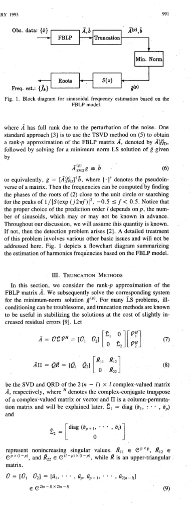
Fig. 1. Block diagram for sinusoidal frequency estimation based on the

FBLP model.

where

A

has full rank due to the perturbation of the noise. One standard approach [3] is to use the TSVD method on (5) to obtain a rank-p approximation of the FBLP matrix

A,

denoted by

A@?,,

followed by solving for a minimum norm LS solution of

g

given by

Ag,g

=

6

(6)

or equivalently,

g

= [A&lt6, where [.It denotes the pseudoin- verse of a matrix. Then the frequencies can be computed'by finding the phases of the roots of (2) close to the unit circle or searching for the peaks of l / ( S ( e x p ( j 2 7 r f ) I 2 , -0.5 5 f

< 0.5. Notice that

the proper choice of the prediction order 1 depends on p , the num-

ber of sinusoids, which may or may not be known in advance. Throughout our discussion, we will assume this quantity is known. If not, then the detection problem arises [2]. A detailed treatment of this problem involves various other basic issues and will not be addressed here. Fig. 1 depicts a flowchart diagram summarizing the estimation of harmonics frequencies based on the FBLP model.

111. TRUNCATION METHODS

In this section, we consider the rank-p approximation of the FBLP matrix

A".

We subsequently solve the corresponding system for the minimum-norm solution

g @ ) .

For many LS problems, ill- conditioning can be troublesome, and truncation methods are known to be useful in stabilizing the solutions at the cost of slightly in- creased residual errors [9]. Let

C ,

0

A = O C P H = [ O ,

4 1 1

0

E,

I[;;]

(7)

An

= QR = [ Q , Q,]

[

3

be the SVD and QRD of the 2(n - 1 ) X 1 complex-valued matrix

A,

respectively, where denotes the complex-conjugate tratspose of a complex-valued matrix or vector and

II

is a column-permuta- tion matrix and will be explained later.

2,

= diag (C,, * * *

,

C p )

and

represent nonincreasing singular values.

R I ,

E

ePxP,

RI,

E C 3 p x ( ' - p ) , and RZ2 E

e('-p)x('-p),

while

R

is an upper-triangular matrix.

992 IEEE TRANSACTIONS ON SIGNAL PROCESSING, VOL. 41, NO. 2, FEBRUARY 1993

and

Q = [Q, Q,] =

[q,,

* *

.

,

qp,

qp+ I )

. . .

, 4 / ] E

c 2 ( " - I ~ x /

all have orthonormal columns, i.e.,

In the absence of noise,

E,

= R,, = 0. Here the permutation matrix

II

= [al,

. . .

, 7r/] is used to represent different methods of performing QRD with column interchanges. Now, we want to preserve as much of the energy as possible (with respect to the Frobenius norm defined below) in the trapezoidal matrix

[I?,

,

RI,]

of (8). Equivalently, we want to leave as little energy as possible residing in the lower right submatrix R,,, which will be truncated.

During the ith stage of the QRD procedure (i = I ,

. . .

, 1 ) , the submatrix R,, has 1 - i

+

1 columns. In the dynamic column- swapping case the column of RZ2 having the largest 2-norm is per- muted into the first column position [9]. This is the column with the maximum linear independence with the subspace defined by

[4,,

. . .

, qi- I]. This process forces the energy in the remaining portion of R2, to be as small as possible. Hence, the subsequent

truncation of R,, results in the smallest possible error.

There are at least three possible methods for determining the per- mutation matrix

II

while performing QRD. They are:

1) For QRD with no pivoting,

II

is simply an identity matrix. We denote this scheme as the TQR method.

2) QRD with preordered columns [6] determines

II

according to a column index maximum-difference bisection rule. Here we select the first and the Ith columns, followed by the column

r(

1

+

1)/21 halfway between 1 and 1. Then we pick the columns that lie in the midway of those ones previously selected, i.e., [(l

+

r ( l

+

1)/21 ) / 2 1 , r ( r ( l

+

1)/21

+

1)/21 , and so on. This selection rule does not depend on the real-time data in

A.

The underlying reason for this ad hoc fixed-ordering scheme is to provide the se- lected columns with a possibly maximum differences or minimum linear dependency among these columns. This ordering scheme is not unique nor is optimum in general. It was motivated due to the nature of the matrix

k

arranged in the form of (3) consisting of perturbed sums of harmonic sinusoids. As an example, suppose there are 5 columns, then the preordering strategy leads to [1]-[5]. Thus we have

II

= [e,, e5, e3, e2, e4], where e; is a dimension 1 column vector with all zero components except for an one at the ith position. We denote this scheme as the TQRR method. It ap- plies only when the frequencies of the input signal components are closely spaced.

3) As for QRD with column pivoting [9, p. 2331,

II

is deter- mined during the QRD process, where s , = ed, and d , E [ l , I ] is the index such that a,,, the d,th column of

k,

has the largest norm. Continuing with this column-pivoting process on the lower right submatrix yet to be triangularized, we can determine the permu- tation matrix

II

which yjelds an optimum QRD column ordering strategy in the sense of preserving most energy in the upper trap- . ezoidal submatrix. However, this

II

is data-dependent and the extra cost for this pivoting may make it less desirable for some appli- cations. We denote this scheme as the TQRP method.

After forcing those weak-rank quantities to be zero and preserv- ing the most significantp-rank, we can obtain a rank-p approximate of

A.

These weak-rank quantities are those entries in the factorized matrix that contribute least significantly to the matrix, or possess the smallest portion of the energy (square of Frobenius norm) of = i j F C j = qYqj = 6,.

the associated matrix. For TSVD,

E,

is discarded and

AEVD

=

8,

c,

r?:.

(12) Similarly, for TQR, the lower right submatrix

I?,,

is discarded and (13) To account for the effect due to truncation, we define the fractional truncated F-norm as

(PI

TQR = [ R l l R , , I '

5") = 1 -

~ ~ A ( ~ ) ~ ~ ~ / \ ~ k ~ ~ ~

(14)

where

11. IIF

is the Frobenius norm given by

I

Thus we have

and

While

0 I 5fVD I

5gRp

5 1 (18)

is valid analytically [9], from extensive computations we also ob- served the relationships among truncated QR methods to satisfy

(19) FTQRP ( P I I STQRR (P) I 5i"dR 5 1.

Therefore, from the point of view of preserving the Frohenius norm (square root of energy) of a matrix, SVD provides the optimum truncation, with TQRP being next, while TQRR and TQR truncate even more (see Fig. 2).

IV. MINIMUM-NORM SOLUTIONS

After truncation, the FBLP LS problem becomes rank-deficient, hence the minimum-norm LS solution is desired in order to sup- press those spurious harmonics in the pseudo-spectrum. For TSVD it is given by

gv,

=

VI

e

;Ioy&.

(20)

After the QRD and truncation of R,,, the FBLP system assumes

IEEE TRANSACTIONS ON SIGNAL PROCESSING, VOL. 41, NO. 2 , FEBRUARY 1993 993 0.3 r Is: 02s-

\

<

.1_____1-__

-

-".-.I_.. 0.2

-

---.-

---._

--_

----

---_

---_

---________

----___

-%_

;

0.15

-

0.1

-

..

Q...

\ .%.,

>----.--

-....>-.

.-... ... _... -x .-. -.- 0.05- \, ..-..---.. .- ... .

---

..._

."-"... -*.

%

45 U, -. i5 Qo 65 io rRII R121g = Ql b (21)

where the matrix on the left is of dimension p X 1, 1

>

p . We

therefore observe the original overdetermined FBLP system of equations given by (3) converted into an underdetermined system. To obtain

g:AR

corresponding to (21), we can perform a QRD on the right of the trapezoidal upper triangular matrix in (13) to zero out and also obtain the orthonormal row space,

PH,

of

[I?,, PI*].

That is

(22)

AFAR

n

= Ql [ R l l

RI,]

=

QILHP."

where = [il,

.

* * ,

41

E e l x p has orthonormal columns and

L H

E C p x p is an upper triangular matrix. This is sometimes called a complete orthogonal factorization [9, p. 2361, and we can consider it as a two-sided direct unitary transformation on a rank-deficient matrix to compress all the energy of a matrix into a square upper triangular matrix. Then from (22) the minimum-norm solution for the underdetermined LS problem

75 follows by 1 -

0

-I5 5 1 -2 -2.5 ( P I .

In summary,

gTQR

in (24) for various TQR methods can be ob- tained in a backward manner. We first perform the QRD and also determine the permutation matrix I1 and the transformed right-hand- side vector Q?

6

as given in (13). After performing another QRD on the truncated upper triangular matrix in (22) we can obtain

F

and

L.

Next, a back substitution for

L-HQr6

followed by a ma- \ria-vector multiplication and a vector permutation results in

g TQR

-

-

-

V . SIMULATION RESULTS

Finally, we present various computer simulations based on the following model. Let f , = cos (27rf, i)

+

cos ( 2 i r - i )

+

w,, i = 1, 2,

.

,

48, withfi = 0.125,

A

= 0.135, 1 = 36 and {w!} is a white Gaussian random sequence. The estimated frequencies,

f,

and

A,

are determined by the phase (from 0 to ?r) of complex roots

closest to the unit circle. For TQRR, we prepermute the columns of the FBLP matrix in the order o f { 1 36 18 9 27 5

.

* * }

as suggested by [6]. We will consider the frequency bias and the standard deviation of the estimated frequency on the evaluation of the performances. Two classes of comparisons will be considered in the following curves. The first one is to compare these truncation methods under various values of SNR from 0 to 50 dB. The second is to observe the asymptotic performance by fixing the order I = 36, and increasing the number of observed data samples. One hundred independent simulations are used to obtain the statistical means and standard deviations.

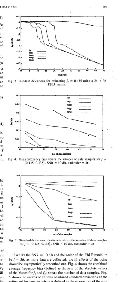
Fig. 2 gives the average fractional truncated Frobenius norms of (15) versus SNR when we preserve only the four most significant ranks of the FBLP matrix for the five different methods. This con- firms their relationships in (18) and (19) and also shows that the truncated energy decreases monotonically as SNR increases. We note that the solid curve for the LS case coincides with the SNR axis due to no truncation at all. Fig. 3 shows the standard deviation offz. We can see the TQRP competes quite well with TSVD, while TQRR performs slightly worse than TQRP but better than TQR without pivoting. 4 . 5 1 . .

.

.

.

.

.

.

.

I

.

.

.

.

.

.

.

.

.

0 5 10 15 20 25 30 35 40 45 50 SNR(dB) -51

'

Fig. 3. Standard deviations for estimatingf, = 0.135 using a 24 X 36

FBLP matrix. -0.5

I

31 I 40 45 50 55 60 65 70 75 no. 01 data s m p h

Fig. 5 . Standard deviations of estimates versus the number of data samples

f o r f = {0.125, 0.135}, SNR = 10 dB, and order = 36.

If we fix the SNR = 1@dB and the order of the FBLP model to be I = 36, as more data are collected, the ill effects of the noise should be asymptotically smoothed out. Fig. 4 shows the combined average frequency bias (defined as the sum of the absolute values of the biases forfl a n d h ) versus the number of data samples. Fig. 5 shows the curves of various combined standard deviations of the estimated frequencies which is defined as the square root of the sum of squares of the standard deviations of each frequency estimate. From Figs. 4 and 5 , it is clear that under moderate SNR conditions,

994 IEEE TRANSACTIONS ON SIGNAL PROCESSING, VOL. 41, NO. 2, FEBRUARY 1993

TABLE I

COMPARISONS OF TRUNCATED LEAST SQUARES METHODS

Freq. Est. Comput. Cost VLSI Updating

TSVD Excellent Very high Complex Difficult

TQRP Very good Medium Medium Medium

TQRR Good Fair Fair Easy

TQR Fair Fair Fair Easy

LS Poor Low Low Easy

the performances of TQRP closely follow that of TSVD. Through- out our simulation, we have fixed the model order 1 = 36. This choice is optimal for the TSVD method. As for the proposed three TQR methods, further investigation and extensive simulations need to be performed to see its effects.

VI. CONCLUS~ONS

Three truncated Q R methods have been proposed for resolving closedly spaced frequencies. Well known for their numerical sta- bility and ease in updating, these TQR methods, at the cost of slightly degraded performance, are promising for real-time appli- cations. Table I summarizes the comparisons among different trun- cation methods. From our simulations, we found that the ratio of flops counts of SVD, Q R with reordering, QR with column pivot- ing, and standard QRD is about 5.9 : 1.1 : 1.1 : 1 . This comparison is based on factorization of a 24 X 36 matrix using PC-MATLAB. We conclude that TQR is the simplest and can be performed easily in a real time updating, but may suffer significant degradation. TQRP provides almost the same performance as SVD, but is not easy to implement in real time processing in that the difficult col- umn reshuffling is required while performing QRD with pivoting. TQRR provides a good compromise between the above two and can also be implemented for systolic array processing. The LS method is simple to implement and update but has a poor frequency estimation capability.

ACKNOWLEDGMENT

The authors would like to thank the reviewers for their valuable comments and suggestions.

REFERENCES

S . Haykin, Adaptive Filter Theory. Englewood Cliffs, NJ: Prentice- Hall, 1986.

S , M. Kay, Modern Spectral Estimation: Theory and Application. Englewood Cliffs, NJ: Prentice-Hall, 1988.

D. W. Tufts and R. Kumaresan, “Estimation of frequencies of mul- tiple sinusoids: Making linear prediction perform like maximum likelihood,” Proc. ZEEE, vol. 70, no. 9 , pp. 975-989, Sept. 1982. M. Kaveh and A. J. Barahell, “The statistical performance of MU- SIC and the minimum norm algorithms in resolving plane waves in noise,” ZEEE Trans Acoust., Speech, Signal Processing, vol. ASSP- 34, no. 2, pp. 331-340, Apr. 1986.

B. D. Rao, “Perturbation analysis of an SVD-based linear prediction method for estimating the frequencies of multiple sinusoids,” IEEE Trans. Acoust., Speech, Signal Processing, vol. 36, no. 7, pp. 1026- 1035, July 1988.

J. P. Reilly, W. G. Chen, and K. M. Wong, “A fast QR-based array- processing algorithm,” Proc. SPZE Znt. Soc. Opt. Eng., pp. 36-47, 1988.

S . L. Marple, Jr., “A tutorial overview of modem spectral estima- tion,” in Proc. ZEEE ZCASSP, 1989, pp. 2152-2157.

[8] W. M. Gentleman and H. T. Kung, “Matrix triangularization by sys- tolic array,” in Proc. SPZEInr. Soc. Opt. Eng., vol. 298, pp. 19-26, 1981.

[9] G. H. Goluh and C. F. Van Loan, Matrix Computations, 2nd ed. Baltimore, MD: Johns Hopkins University Press, 1989.

[IO] J . R. Bunch and C. P. Nielsen, “Updating the singular value decom- position,” Numer. Math., vol. 31, pp. 111-129, 1978.

[ l l ] P. Comon and G. H. Golub, “Tracking a few extreme singular values and vectors in signal processing,” Proc. ZEEE, vol. 78, no. 8, pp. 1327-1343, Aug. 1990.

The Double Bilinear Transformation for 2-D Systems

in State-Space Description

P. Agathoklis

Abstract-The double bilinear transformation for two-dimensional (2-D) systems described by state-space models is considered. The re- lationships between the realization matrices of the continuous and the discrete 2-D transfer functions are presented.

I. INTRODUCTION

The bilinear transformation has been widely used to transform continuous prototypes into discrete transfer functions. For one-di- mensional (1-D) systems it has been studied for systems described by transfer functions, as well as by state-space models [l], and has been used in many filter design techniques and control design ap- plications. In the two-dimensional (2-D) case, the double bilinear transformation has been used to design 2-D digital filters ([4], [5] are examples of such techniques), as well as for double integral evaluations [2] of systems described by transfer functions.

In this correspondence, the double bilinear transformation for 2-D systems described by state-space models is considered. The relationships between the realization matrices of the discrete and the continuous transfer functions are given.

11. PRELIMINARIES

Consider a 2-D discrete system represented by a 2-D state-space model [3]:

where x h E R“ and XI’ E R” represent the horizontal and vertical states respectively, U is the input and y the output. The system transfer matrix is given by

Manuscript received March 12, 1992; revised June 6, 1992. This work The author is with the Department of Electrical and Computer Engi- IEEE Log Number 92051 19.

was supported by the NSERC.

neering, University of Victoria, Victoria, B. C., V8W 3P6, Canada.