Ling-Yuan Hsu
e-mail: lance1214@gmail.com
Tsung-Lin Chen
1e-mail: tsunglin@mail.nctu.edu.tw
Department of Mechanical Engineering, National Chiao Tung University, Hsinchu, Taiwan 30010, R.O.C.
Estimating Road Angles With the
Knowledge of the Vehicle Yaw
Angle
This paper presents a method of estimating road angles using state observers and three types of sensors (lateral acceleration sensors, longitudinal velocity sensors, and suspen-sion displacement sensors). The proposed method differs from those in most existing literature in three aspects. First, a “full-state” vehicle model is used to describe nonlin-ear vehicle dynamics on a sloped road. Second, “switching observer” techniques are used to suggest suitable sensors and to construct state observers. Lastly, the road angles are described by three Euler angles, and two of them are estimated simultaneously. The analysis indicates that (1) road angles affect vehicle dynamics through components of the gravitational force acting on the vehicle body. These gravitational forces can be correctly estimated with an estimation accuracy less than 7.5%, even when road angles vary with time. (2) Those road angles can be correctly estimated only when the vehicle yaw angle is known. 关DOI: 10.1115/1.4001330兴
1 Introduction
Many research reports have shown that road angles have direct influences on vehicle dynamics, and those effects need to be iden-tified for a satisfactory performance. For example, lacking of road information, rollover prediction systems may produce false alarms 关1,2兴; vehicle stability controls may either initiate false activation or need large actuation power关3,4兴. The road angle problems are difficult to tackle with because it is neither practical to assume that road angles can be obtained beforehand, nor measure them in real time using sensors attached to a vehicle body. Road angles are difficult to measure in real time because they are often coupled with other vehicle dynamics in sensor measurements, such as ve-hicle roll/pitch angles, lateral accelerations, etc.关5–8兴.
In general, road angles are described by the “road curve angle,” “road bank angle,” and “road grade angle,” as shown in Fig. 1. Even though the road bank/grade angle and the vehicle roll/pitch angle have indistinguishable influences on sensor measurements, they play very different roles in vehicle dynamics. Therefore, some researchers proposed using vehicle dynamics and state ob-server techniques to estimate road angles 关3,7,9兴. In order to achieve a reliable estimation of road angles with less amount of sensor deployments, the incorporated vehicle model must be as precise as possible; this leads to high-order, nonlinear differential equations for vehicle modeling. Some conventional nonlinear ob-server design methods, such as the extended Kalman filter共EKF兲, require information from the Jacobian matrices of system equa-tions and measurement equaequa-tions at each sampling time关10兴. To construct such an observer for an n-state, m-output nonlinear sys-tem, one needs to derive/code共n⫻n+m⫻n兲 equations by hand. For high-order nonlinear vehicle systems, this is impractical. Partly for that reason, most road angle estimation systems employ more amounts of sensors to work with simplified vehicle models 关3,7–9,11兴.
In most road angle estimation literature, the coordinate systems were defined in a way that the road curve angle was aligned with the vehicle yaw angle. And the estimations were performed on either road bank angle关4,3,6,8兴 or road grade angle 关9,12兴; only a
few on those two angles simultaneously 关7,5,11兴. And, in those two-angle estimations, the road bank angle and grade angle were both referred to the same coordinate, which is totally different from the conventional “Euler angle” approach关13兴. Consequently, even one knows the heading direction of a vehicle 共vehicle yaw angle兲, it is still difficult to picture 共calculate兲 the road terrain from the values of their road bank angle and road grade angle.
Previously, the author proposed a novel switching computation scheme 关2兴, which can solve differential equations numerically. With that method, a set of high-order differential equations is separated into two sets of low-order differential equations. These two sets of low-order differential equations calculate state values in a way similar to “domain decomposition methods关14兴.” The state values obtained from this method can be fairly close to those of the analytical solutions. The analysis of stability and conver-gence 关1兴 indicates that, by choosing a proper “switching time,” the computation accuracy is proportional to the switching time to the power of 2. This method can be extended to the state observer construction for high-order nonlinear systems with the benefit of reducing a large amount of equation derivations.
In this paper, we present a novel approach to estimate road bank angle, road grade angle, and their effects on vehicle dynamics. In this method, estimating road angles needs the information of ve-hicle yaw angle but estimating the road angle effects does not. Unlike other approaches in this aspect, the conventional Euler angle is used to describe a road terrain, and the referenced coor-dinate system is fixed on Earth. Thus, the description of terrain is intuitive and independent of the vehicle yaw angle. Since the es-timation of road angles is achieved by the angle influence on vehicle dynamics, a “full-state” vehicle model共22 states, nonlin-ear differential equations兲 is incorporated to ensure the estimation accuracy under various vehicle maneuvers. As discussed before, using such a high-order nonlinear model in state estimations would require lots of equation derivations. Therefore, the previ-ously proposed switching computation techniques are used to sug-gest suitable sensors and to reduce the amount of equation deri-vations. The procedures of constructing the estimation system and the observability analysis of road angle estimations are both dis-cussed in detail in this paper.
2 Vehicle Model
2.1 Coordinate Systems and Euler Angles. Two sets of Eu-ler angles and four coordinate systems shown in Fig. 2 are
intro-1
Corresponding author.
Contributed by the Dynamic Systems Division of ASME for publication in the JOURNAL OFDYNAMICSYSTEMS, MEASUREMENT,ANDCONTROL. Manuscript received October 29, 2008; final manuscript received December 10, 2009; published online April 14, 2010. Assoc. Editor: J. Karl Hedrick.
duced for constructing the vehicle model. These four coordinate systems are global frame兵g其, road frame 兵r其, body frame 兵b其, and auxiliary frame兵a其. Similar to conventional approaches, the global frame is fixed to a point on Earth, whereas the body frame is fixed to the center of gravity共CG兲 of the vehicle. In addition to con-ventional approaches, the road frame is introduced to describe vehicle dynamics on a sloped road. The relationship between the road frame and the global frame is described by the Euler angles 共r,r,r兲, which are referred to as the road grade angle, road bank angle, and road curve angle, respectively. The relationship between the road frame and the body frame is described by an-other set of Euler angles共,,兲. These three angles describe the vehicle attitude relative to the road level and are referred to as the “vehicle yaw angle,” “vehicle pitch angle,” and “vehicle roll angle,” respectively. Since the vehicle may move along a path irrelevant to road curve angles, the road curve angle does not affect the vehicle dynamics. Thus, it is assumed to be zero 共r = 0兲 in this paper.
The auxiliary frame 共aux-frame兲 is obtained by rotating the
z-axis of the road frame until the x-axis of the road frame is
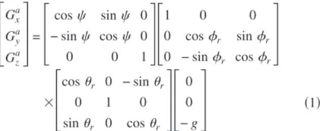
aligned with the x-axis of the body frame. The aux-frame is used because it describes the vehicle translational motions in an intui-tive manner while preserving the information of other vehicle dy-namics relative to the road level. In the following vehicle model-ing, vehicle translational motions are described in the aux-frame, and the rotational motions are described by Euler angles共,,兲. 2.2 Road Angle Effects and Vehicle Modeling. As shown in Fig. 1, Earth’s gravity is an external force acting on the vehicle body and is fixed to the global frame. Therefore, it affects vehicle dynamics via road angles. If the sloped road is described by the Euler angles 共r,r,r兲 with the rotation order of “pitch-roll-yaw” and the road curve angle is zero共r= 0兲, three components of the gravitational force, presented in the aux-frame共Gxa, Gya, Gza兲, can be obtained as
冤
Gxa Gya Gz a冥
=冤
cos sin 0 − sin cos 0 0 0 1冥冤
1 0 0 0 cosr sinr 0 − sinr cosr冥
⫻冤
cosr 0 − sinr 0 1 0 sinr 0 cosr冥冤
0 0 − g冥
共1兲 where g is Earth’s gravity. Since Earth’s gravity is the only exter-nal force that is fixed to the global frame in most cases, the “road angle effects” on vehicle dynamics can be attributed to these gravitational forces共Gxa, Gya, Gza兲.Similar to other researches关15,16兴, the vehicle modeling is pro-ceeded with the “sprung mass system” and “unsprung mass sys-tem.” Assuming that the vehicle body is rigid, the dynamics of the sprung mass system, presented in the aux-frame, is
mtot共x¨a− y˙a˙兲 =
兺
F x,tire a + mtotGxa mtot共y¨a+ x˙a˙兲 =兺
F y,tire a + mtotGya mtotz¨a=兺
F z,spring a + mtotGza ¨ = ¨ sin + ˙˙ cos + M¯ x ¨ = − ˙˙ cos + M¯ ycos − M¯zsin ¨ = ˙˙ sec + ˙˙ tan + M¯ysin sec + M¯zcos sec
M¯x= Mx
Ix
−Iz− Iy
Ix
共˙ cos + ˙ cos sin 兲共− ˙ sin +˙ cos cos 兲 M¯y= My Iy −Ix− Iz Iy
共˙ − ˙ sin 兲共− ˙ sin + ˙ cos cos 兲
M¯z= Mz
Iz
−Iy− Ix
Iz
共˙ − ˙ sin 兲共˙ cos + ˙ cos sin 兲 共2兲 where the superscript a indicates state values represented in the aux-frame; xa, ya, and zaare the translational displacements of the vehicle CG; Fx,tirea , Fy,tirea , and Fz,springa are the translational forces (a) {b} {b} {g} {g} {r} {b} (b) (c) O road centerline {r} {r} {g} x x x x y y y y z z z z x z y z x y r ψ ψ r φ θr g mtot mtotg
Fig. 1 A vehicle on a sloped road:„a… the road curve angler,
„b… the road bank angler, and„c… the road grade angler
sprung mass {g} {b} 4 4 1 1 unsprung mass {a} CG y y y z z z x x x road centerline x z y {r} h f t 2 r t 2 r l f l 2 2 3 3 global frame road frame aux-frame body frame b,1 F a,1 F a tire,1 y, F a tire,1 x, F x y {a} b,1 F a,1 F a tire,1 y, F a tire,1 x, F x y {a}
Fig. 2 Four coordinate systems for the vehicle modeling.ˆg‰: global frame,
generated by tires and suspension systems; Mx, My, and Mz are the external torques acting on the vehicle CG along three axes of the body frame; and Ix, Iy, and Izare the moments of inertia of the sprung mass system along three axes of the body frame. The dy-namics of the unsprung mass system, presented in the aux-frame, is
Iw,i˙i a
= − re,iFa,i− Tb,i+ Tm,i 共i = 1 – 4兲
H˙1a= − z˙a+ lf˙ cos + tf共˙ sin sin − ˙ cos cos 兲 H˙2a= − z˙a+ l
f˙ cos − tf共˙ sin sin − ˙ cos cos 兲 H˙3a= − z˙a− lr˙ cos − tr共˙ sin sin − ˙ cos cos 兲 H˙4a= − z˙a− l
r˙ cos + tr共˙ sin sin − ˙ cos cos 兲 共3兲 where ia represents the angular rate of each tire i; Fa,i is the longitudinal adhesive force generated by tire i; Tb,i and Tm,iare the braking and traction torque transmitted to tire i, respectively;
Iw,iis the moment of inertia of tire i; re,iis the effective rolling radius of tire i; Hiarepresents the displacement of each suspension corner i; the subscript i refers to four suspension corners in a way: 1→front-left, 2 to 4 in a clockwise motion; lf and lr are the distances from the CG to the front and rear axes, respectively; and
tf and trare one-half the distances of the front and rear tracks, respectively. More details of this vehicle modeling can be found in Refs.关1,2兴.
3 Road Angle Estimations
In this paper, two road angles 共r,r兲 are treated as system states and identified by state observer techniques. In order to ap-ply existing observer algorithms to this problem, the “dynamic equations” of road angles should be obtained prior to the observer construction. However, it is neither practical to use sensors, at-tached to a vehicle body, to measure the change rate of road angles, nor to obtain this information for a specific road terrain. The change rates of these two angles are assumed to be zeros for now 共Eq. 共4兲兲. Although this assumption leads to model errors when the vehicle is moving on a road with varying road angles, this error can be alleviated using some robust observer designs, which will be discussed shortly.
˙r= 0
˙r= 0 共4兲
From Eqs.共1兲–共4兲, one can obtain a 22-state vehicle model that can mimic vehicle behaviors on a sloped road. This vehicle model is used to construct the state observer for estimating road angles and their effects.
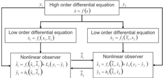
3.1 Switching Observer Scheme. As discussed before, using the conventional EKF to construct an observer for a 22-state non-linear system, one must derive 484 partial derivative terms 共22 ⫻22=484兲. Moreover, to examine the feasibility of a sensor can-didate, one must derive at least 22 derivative terms. It is difficult to do so. The switching observer scheme 关2兴, developed from a switching computation scheme, is used to suggest suitable sensors and reduce the intensive equation derivations. In that case, one can then design two individual observers; one observer requires 144 partial derivative terms while the other requires 100 partial derivative terms. The amount of derivations is roughly one-half of that required for the conventional EKF. As shown in Fig. 3, the switching observer scheme is operated in a way that, within each switching cycle, one observer estimates state values while the other observer is held static. They switch their roles in the next switching cycle.
3.2 Vehicle Yaw Model and Vehicle Roll Model. Following the concepts of switching computation scheme, this 22-state ve-hicle model is separated into a 12-state submodel 共关˙,,x˙a, xa, y˙a, ya,1–4a ,r,r兴T兲 and a 10-state submodel 共关˙,,˙,,z˙a, za, H1–4a 兴T兲. They are referred to as the vehicle yaw model and vehicle roll model in this paper.
Vehicle yaw model:
¨ = ˙˙ sec + ˙˙ tan + M¯
ysin sec + M¯zcos sec x¨a= y˙a˙ +
兺
Fx,tirea /mtot+ Gxa y¨a= − x˙a˙ +
兺
F y,tire a /mtot+ Gy a Iw,i˙i a= − re,iFa,i− Tb,i+ Tm,i
˙r= 0
˙r= 0 共5兲
Vehicle roll model:
¨ = ¨ sin + ˙ ˙ cos + M¯ x ¨ = − ˙˙ cos + M¯ ycos − M¯zsin z¨a=
兺
Fz,springa /mtot+ Gz aH˙1a= − z˙a+ lf˙ cos + tf共˙ sin sin − ˙ cos cos 兲 H˙2a= − z˙a+ l
f˙ cos − tf共˙ sin sin − ˙ cos cos 兲 H˙3a= − z˙a− lr˙ cos − tr共˙ sin sin − ˙ cos cos 兲 H˙4a= − z˙a− lr˙ cos + tr共˙ sin sin − ˙ cos cos 兲 共6兲 According to Eqs.共1兲 and 共2兲, road angles have a direct impact on three translational accelerations. For the accuracy of state estima-tion, the “dynamics” of two road angles reside in the vehicle yaw model because the vehicle yaw model contains more translational dynamics than the vehicle roll model.
Note that this is not the only way of splitting a vehicle system. From the stability analysis of the switching computation scheme, the system共states兲 splitting can be done differently as long as it satisfies certain stability constraints关1兴.
3.3 Sensor Selection. According to Eq. 共2兲, the road angle affects vehicle dynamics in many aspects. Therefore, in order to correctly estimate road angles from vehicle dynamics, most ve-hicle states must be known or correctly estimated. For this reason,
High order differential equation
Low order differential equation Low order differential equation
( )x f x =& ( 1 2) 2 2 f x, x x =& (1 2) 1 1 f x, x x =& Nonlinear observer
( )
( )( )
1 2 1 1 1 1 1 2 1 1 1 ˆ , ˆ ˆ ˆ ˆ , ˆ ˆ x x h y y y L x x f x = − + = & Nonlinear observer( )
( )( )
1 2 2 2 2 2 2 2 1 2 2 ˆ , ˆ ˆ ˆ ˆ , ˆ ˆ x x h y y y L x x f x = − + = & 1 y y2 1 ˆx 2 ˆxFig. 3 A diagram of the switching observer scheme. One
ob-server estimates state values within a switching cycle while the other is held static. They switch their roles of estimating state values in the next cycle.
sensors are chosen to ensure that most of the 22 vehicle states are observable. Here, we choose lateral acceleration sensors, longitu-dinal velocity sensors, and four suspension displacement sensors for this estimation system. Although longitudinal velocity sensors are not popular in commercial vehicles, a global positioning sys-tem 共GPS兲/inertial navigation system 共INS兲 sensor system can provide the information of the longitudinal velocity关17,18兴. How-ever, the output of the GPS/INS systems needs lots of signal
pro-cessing to obtain the velocity information, and is beyond the scope of this paper. We assume that the longitudinal velocity sen-sor is available for simplicity.
When adapting the switching observer scheme, the lateral ac-celeration sensors and longitudinal velocity sensors共Y1in Eq.共7兲兲 work with the state observer of the vehicle yaw model, while the four suspension displacement sensors共Y2in Eq.共8兲兲 work with the state observer of vehicle roll model.
Y1=
冋
y¨m g x˙ma册
=冋
共x¨a− y˙a˙ + G x a兲sin sin + 共y¨a+ x˙a˙ + G y a 兲cos + 共z¨a+ G z a 兲sin cos x˙a
册
共7兲 Y2=冤
H1,ma H2,ma H3,ma H4,ma H1,ma H2,ma H3,ma H4,ma冥
=冤
H1a H2a H3a H4a − za+ lfsin − tfcos sin − za+ lfsin + tfcos sin − za− l
rsin + trcos sin − za− l
rsin − trcos sin
冥
共8兲
Note that there are duplicated output equations in Y2 and they share the same values from corresponding sensor measurements
Hi,ma . This is because the suspension displacement Hiais either a redundant or independent state depending on whether the tire i is on or off the ground 关2兴. Once a tire is identified to be off the ground, its duplicated equation is removed as it is no longer valid. For example, if the first tire is identified to be off the ground, the fifth equation in Y2is removed. These duplicated equations ensure the success of state estimation no matter tires are on or off the ground.
3.4 Observer Algorithm. The observer algorithms are chosen to be the EKF because it is simple and effective in the sensor noise reduction. Although the EKF has been questioned for the state convergence 关10兴; in that case, one can use the iterative Kalman filter 共IKF兲 to obtain both noise reduction and state convergence.
As discussed before, the assumption of constant road angles 共Eq. 共4兲兲 may lead to modeling error for state estimations. Nor-mally, the model error can be dealt with by two methods in Kal-man filtering: One adds large fictitious noise to dynamic equations 关10兴, and the other one uses robust observer design such as “fad-ing memory techniques关19,20兴.” The fading memory technique is done by introducing a “forgetting factor” into the computation of the “predicted covariance matrix” in EKF关10兴. The predicted co-variance matrix is then increased; thus the observer would believe more in sensor outputs than in system models. The forgetting factor can be chosen in a way that optimizes the performance of state convergence and noise reduction 关19,20兴. However, the equation derivation is beyond the scope of this paper and thus omitted. Hence, the EKF accompanied with fading memory tech-niques is utilized in this paper.
4 Observability Analysis
The success of state estimations depends on the system observ-ability. And the local observability of a nonlinear system is deter-mined by the rank of the observability matrix, which is comprised
of partial derivatives of the measurement equations and their de-rivatives关21兴. In this vehicle system, the observability matrix can be written as Wo⬅ 䉮
冋
冋
Y1 Y2册
,冋
Y˙1 Y˙2册
,冋
Y ¨ 1 Y¨2册
, ¯册
T 共9兲 As discussed before, this estimation system is designed to en-sure most of vehicle states converging to their correct values. For better understanding of the system observability, the observability analysis is proceeded for road angles first and then for the entire vehicle states.4.1 Observability Analysis for Road Angles. The road angles共r,r兲 affect vehicle dynamics only through three gravi-tational forces共Gxa, Gya, Gza兲. Thus, these gravitational forces must be observable for the possible observability of road angles. There-fore, the observability of gravitational forces is examined first. With those selected sensors, the observability of gravitational forces can be determined by the following matrix:
Wo,gravity= Ga
冋
冋
Y1 Y2册
,冋
Y ˙ 1 Y˙2册
,冋
Y ¨ 1 Y¨2册册
T =冤
2 sinsin 2 cos 2 sincos
0 0 0 08⫻1 08⫻1 08⫻1 y¨m g x˙a y¨m g y˙a y¨m g z˙a 1 0 0 08⫻1 08⫻1 08⫻1
冉
x¨a x˙a+ y¨a x˙a冊
y¨m g x˙a冉
x¨a y˙a+ y¨a y˙a冊
y¨m g y˙a冉
z¨a z˙a+ 1冊
y¨m g z˙a 0 0 0 08⫻1 08⫻1 18⫻1冥
Ga=关
Gx a , Gy a , Gz a兴
T 共10兲 The rank of the above matrix can be 3 but it depends on the state values of other vehicle dynamics. Meaning that if those vehicle states can be measured or correctly estimated, three gravitational forces can be correctly estimated.The observability of three angles共r,r,兲 that parametrized gravitational forces in Eq.共1兲 can be calculated by “chain-rules” techniques
Wo,angle= 兵r,r,其
冋
冋
Y1 Y2册
,冋
Y ˙ 1 Y˙2册
,冋
Y ¨ 1 Y¨2册
, ¯册
T = 兵Ga ,G˙a,¯其冋
冋
Y1 Y2册
,冋
Y ˙ 1 Y˙2册
,冋
Y ¨ 1 Y¨2册
, ¯册
T · G G⬅ 兵r,r,其关
Ga , G˙a, ¯兴
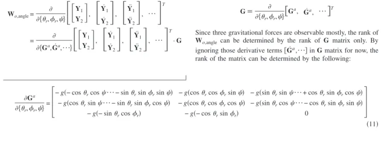
TSince three gravitational forces are observable mostly, the rank of Wo,angle can be determined by the rank of G matrix only. By ignoring those derivative terms关G˙a,¯兴 in G matrix for now, the rank of the matrix can be determined by the following:
Ga 兵r,r,其
=
冤
− g共− cosrcos ¯ − sin rsinrsin兲 − g共cos rcosrsin兲 − g共sin rsin ¯ + cos rsinrcos兲 − g共cosrsin ¯ − sin rsinrcos兲 − g共cos rcosrcos兲 − g共sin rcos ¯ − cos rsinrsin兲
− g共− sinrcosr兲 − g共− cosrsinr兲 0
冥
共11兲
It can be shown that the above matrix is unconditionally singular and its rank is 2. In that case, according to Ref.关22兴, including more derivative terms共关G˙a,
¯兴兲 would not increase the rank of the observability matrix G.
4.2 Observability Analysis for Vehicle Dynamics. The ob-servability of the overall vehicle system共22 states兲 is examined to show if those state values can be correctly obtained. Because of the switching observer scheme, the observability is checked for the vehicle yaw model and vehicle roll model separately.
4.2.1 Vehicle Yaw Model. Before examining the rank of the
observability matrix of the vehicle yaw model, we first check the partial derivatives of the measurement equations共Y1兲 and its de-rivatives with respect to the states of longitudinal displacement 共xa兲 and lateral displacement 共ya兲.
xa
冤
Y1 Y˙1 ]冥
= ya冤
Y1 Y˙1 ]冥
=冤
0 0 ]冥
n⫻1 共12兲 Equation共12兲 reveals that the associated partial derivatives are all zeros, and thus the longitudinal displacement and lateral displace-ment are globally unobservable. This result can be understood by the fact that displacement information cannot be obtained by nei-ther acceleration sensors nor velocity sensors.The rank of the observability matrix of the vehicle yaw model is difficult to calculate analytically because it requires lots of equation derivations. In this case, a trajectory of the vehicle states is specified and the rank of the observability matrix is calculated numerically. The simulation results show that the rank of the ob-servability matrix is 9. Since共i兲 all the elements in Eq. 共12兲 are zeros,共ii兲 three gravitational forces are observable 共Eq. 共10兲兲, and 共iii兲 the observability matrix of three angles 共r,r,兲 loses one rank 共Eq. 共11兲兲, one can conclude that, except the longitudinal displacement, lateral displacement, and one angle from共r,r,兲, the rest of states in the vehicle yaw model are all observable along this special trajectory.
4.2.2 Vehicle Roll Model. For simplicity, we check the
observ-ability of the vehicle roll model using measurement equations Y2 and their first derivatives only, which leads to the following:
Wo,roll=䉮
冋
Y2 Y˙2册
=冋
04⫻6 I4⫻4
A12⫻6 012⫻4
册
16⫻10 共13兲where I is an identity matrix. One can prove that the rank of the lower-left matrix A is 6, except at=90 deg. Thus, all states in the vehicle roll model are observable except when the vehicle
pitch angle is 90 deg. Furthermore, the derivation indicates that the rank of the observability matrix can still be 10 when two of the duplicated measurement equations in Eq. 共8兲 are removed from the observability matrix. This finding suggests that two of those duplicated measurement equations are redundant for state estimation. However, since it is impossible to know in advance which tire would lift off, all four duplicated measurement equa-tions are used.
Since the vehicle states appearing in Wo,gravityare all observ-able and the Wo,gravity matrix is nonsingular, it is possible to choose a suitable observer algorithm to correctly estimate three gravitational forces. On the other hand, since the rank of the ob-servability matrix Wo,angleis 2, those three angles共r,r,兲 can be correctly estimated only when one of them is known. 5 Numerical Simulation
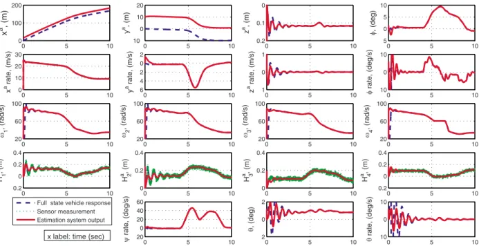
The following simulations are meant to validate the feasibility of the proposed method. In these simulations, the vehicle moves at an initial longitudinal speed of 25 m/s and then the steering wheel makes a left-hand turn, as shown in Fig. 4. For simplicity, the noises associated with all the integrated sensors共lateral accelera-tion sensor, longitudinal velocity sensor, and suspension displace-ment sensors兲 are assumed to be white, and their standard devia-tions are 0.08 m/s2, 0.01 m/s, and 0.01 m, respectively. Simulation results are shown in Figs. 5–11. The state values from
0 2 4 6 8 10 0 20 40 60 80 100 120 140 160 180 Time, (sec) deg Steering angle
the full-state vehicle model are shown in dashed-blue lines and represent real vehicle dynamics. The state values from the sensor output equation are shown in dotted-green lines and represent real sensor measurement. The state values from the proposed estima-tion system are shown in solid-red lines. Both the sampling time of the system and the switching time of the switching observers are set at 0.001 s.
Case I shows a vehicle moving on a road with the road bank angle of 5 deg and road grade angle of⫺5 deg. As shown in Fig. 5, the estimation system can estimate most vehicle dynamics cor-rectly, except for the longitudinal displacement 共xa兲 and lateral displacement共ya兲. Also, as shown in Fig. 6, the estimation system can estimate three gravitational forces correctly but fails to esti-mate three angles共r,r,兲. These simulation results agree very well with the analysis shown in Sec. 4.
These results can be further verified by the singular values of the corresponding observability matrix. The observability matrices of gravitational force 共Wo,gravity兲 and of angle estimations 共Wo,angle兲 are calculated at each sampling time, and their
corre-sponding singular values are drawn in Fig. 7. All singular values are nonzero for the gravitational forces, and thus the estimations of these forces are correct. On the other hand, because one of the singular values for road angles is zero, the estimations of those angles are erroneous. Furthermore, the relative accuracy 共⬅共estimated value−real value兲/共real value兲 关23兴兲 of the gravi-tational force estimation is on average of 0.22%, 0.14%, and 0.006% for Gxa, Gya, and Gza, respectively.
Case II shows a vehicle moving on a road. The conditions in this case are the same as those in Case I, except that the sensor system provides additional measurements: vehicle yaw angle with a standard deviation of 0.01 rad. As shown in Fig. 8, the estima-tion system can estimate accurately for three gravitaestima-tional forces as well as for three angles共r,r,兲. This simulation results agree with the arguments shown in Sec. 4. The relative accuracies of state estimations are 0.48%, 0.64%, and 0.55% forr,r, and, and 0.82%, 0.42%, and 0.003% for Gxa, Gya, and Gza.
0 5 10 0 100 200 x a , (m) 0 5 10 10 0 10 20 y a, (m) 0 5 10 0.2 0.1 0 z a, (m) 0 5 10 0 10 20 30 x arate, (m/s)
Full state vehicle response Sensor measurement Estimation system output
0 5 10 6 4 2 0 2 y arate, (m/s) 0 5 10 1 0 1 z arate, (m/s) 0 5 10 5 0 5 10 φ, (deg) 0 5 10 10 0 10 φ rate, (deg/s) 0 5 10 2 0 2 θ, (deg) 0 5 10 10 0 10 θ rate, (deg/s) 0 5 10 20 0 20 40 60 ψ rate, (deg/s) 0 5 10 20 60 100 ω1 , (rad/s) 0 5 10 20 60 100 ω2 , (rad/s) 0 5 10 20 60 100 ω3 , (rad/s) 0 5 10 20 60 100 ω 4 , (rad/s) 0 5 10 0.2 0 0.2 0.4 H a,1 (m) 0 5 10 0 0.2 0.4 H a, 2 (m) 0 5 10 0 0.2 0.4 H a ,3 (m) 0 5 10 0.2 0 0.2 0.4 H a,4 (m)
x label: time (sec)
Fig. 5 Estimating vehicle dynamics for Case I. The estimation system can estimate most vehicle dynamics correctly,
except for longitudinal displacement xaand lateral displacement ya.
0 2 4 6 8 10 1 0 1 2 m/s 2
Longitudinal component of gravity
Full state vehicle response Estimation system output
0 2 4 6 8 10 2 1 0 1 2 m/s 2
Lateral component of gravity
0 2 4 6 8 10 9.7 9.75 9.8 Time, (s) m/s 2
Vertical component of gavity
0 2 4 6 8 10 50 0 50 100 150 deg
Vehicle yaw angle
0 2 4 6 8 10 0
5 10
deg
Road bank angle
0 2 4 6 8 10 10 5 0 Time, (s) deg
Road grade angle
Fig. 6 Estimating road angles and their effects for Case I. The
estimation system can estimate three gravitational forces accu-rately but fails to estimate three angles.
0 1 2 3 4 5 6 7 8 9 10 0 2 4 6 8 10 Time, (sec) S ingular value
Observability matrix for gravitational force estimation
0 1 2 3 4 5 6 7 8 9 10 0 5 10 15 Time, (sec) S ingular value
Observability matrix for angle estimation
first singular value second singular value third singular value first singular value
third singular value second singular value
Fig. 7 Singular values of the observability matrices for
gravi-tational force estimations and for angle estimations. None of the singular value of the gravitational force estimation is zero. One of the singular values of the angle estimation is zero along the entire trajectory.
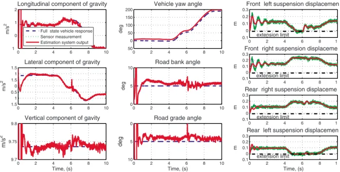
Case III shows a vehicle moving on a road. The conditions in this case are the same as those in Case I, except that the maximum steering wheel angle is 270 deg. As shown in Fig. 9, the estima-tion system can obtain correct values for three gravitaestima-tional forces, even when two suspensions reach their extension limits 共dashed-dotted line兲 from 5.2 s to 6.1 s. This implies that the estimation system can still work well when two tires are off the ground. The relative accuracy of the gravitational force estimation is on average of 4.11%, 7.16%, and 0.004% for Gxa, Gay, and Gza, respectively. The estimation accuracy in this case is worse than that in Case I. This is because the duplicated equations in Eq.共8兲 are removed when tires are off the ground, and that lowers the degree of observability for Gxa, Gya, and Gzaestimation.
Case IV shows a vehicle moving on a road with which the road bank angle and road grade angle are both changing with time. In this simulation, two angles are sinusoidal with the frequency of 0.25 Hz and the magnitude of 10 deg. As shown in Fig. 10, the estimation system can still obtain correct values for three
gravita-tional forces. The relative accuracies of the gravitagravita-tional force estimation are 0.92%, 5.95%, and 0.044% for Gxa, Gya, and Gzaon average. The estimation accuracy in this case is roughly the same as the case of constant angles. It can be attributed to that the fading memory techniques are in effect to optimize the perfor-mance of state convergence and estimation accuracy.
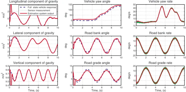
Case V shows a vehicle moving on a road. The conditions in this case are the same as those in Case IV, except that the sensor system provides three additional information: vehicle yaw rate, road bank rate, and road grade rate. These information can be obtained by attaching gyroscopes to the vehicle body. For simplic-ity, the standard deviations of these measurements are all assumed to be 0.01 rad/s. As shown in Fig. 11, the estimation system can obtain correct values for three gravitational forces, three angular rates, but still fails on three angles. The explanation for this case is shown in Sec. 6. 0 2 4 6 8 10 1 0 1 2 m/s 2
Longitudinal component of gravity
0 2 4 6 8 10 2 1 0 1 2 m/s 2
Lateral component of gravity
0 2 4 6 8 10 9.7 9.75 9.8 Time, (s) m/s 2
Vertical component of gavity
0 2 4 6 8 10 50 0 50 100 150 deg
Vehicle yaw angle
Full state vehicle response Sensor measurment Estimation system output
0 2 4 6 8 10 0
5 10
deg
Road bank angle
0 2 4 6 8 10 10 5 0 Time, (s) deg
Road grade angle
Fig. 8 Estimating road angles and their effects for Case II. The
estimation system can estimate three gravitational forces and three angles accurately with the additional information of ve-hicle yaw angle.
0 2 4 6 8 10 1 0 1 2 m/s 2
Longitudinal component of gravity
0 2 4 6 8 10 1.5 1 0.5 0 1.5 1 1.5 m/s 2
Lateral component of gravity
0 2 4 6 8 10 9.7 9.75 9.8 Time, (s) m/s 2
Vertical component of gavity
0 2 4 6 8 10 50 0 50 100 150 200 deg
Vehicle yaw angle
0 2 4 6 8 10
0 5 10
deg
Road bank angle
0 2 4 6 8 10 10 5 0 Time, (s) deg
Road grade angle
0 2 4 6 8 1 0.1 0 0.1 0.2 0.3 m
Front left suspension displacemen
Full state vehicle response Sensor measurement Estimation system output
0 2 4 6 8 1 0.1 0 0.1 0.2 0.3 m
Front right suspension displaceme
0 2 4 6 8 1 0.1 0 0.1 0.2 0.3 m
Rear right suspension displaceme
0 2 4 6 8 1 0.1 0 0.1 0.2 0.3 m Time, (s)
Rear left suspension displacemen extension limit
extension limit
extension limit
extension limit
Fig. 9 Estimating road angle and their effects for Case III. The suspension displacement plots„the third column… indicate
that the front-left and rear-left tires are off the ground. The estimation system can still estimate three gravitational forces accurately. 0 2 4 6 8 10 5 0 5 m/s 2
Longitudinal component of gravity
Full state vehicle response Estimation system output
0 2 4 6 8 10 3 2 1 0 1 2 m/s 2
Lateral component of gravity
0 2 4 6 8 10 9 9.5 10 Time, (s) m/s 2
Vertical component of gavity
0 2 4 6 8 10 50 0 50 100 150 deg
Vehicle yaw angle
0 2 4 6 8 10 15 5 5 15 deg
Road bank angle
0 2 4 6 8 10 15 5 5 15 Time, (s) deg
Road grade angle
Fig. 10 Estimating road angles and their effects for Case IV.
The estimation system can estimate three gravitational forces accurately when the road angles vary as sinusoidal waves.
6 Discussion
Simulation results 共Figs. 6 and 8兲 and observability analysis 共Sec. 4兲 both indicate that three gravitational forces can be cor-rectly estimated but three angles 共r,r,兲 cannot. Since those three angles affect vehicle dynamics only through gravitational forces and their dynamics are assumed to be static共Eq. 共4兲兲, esti-mating three angles is essentially the same as solving Eq. 共1兲. According to “Wahba’s problem 关24兴,” the information of two vectors represented in both a fixed frame and a rotated frame is needed to determine three angles in a rotation matrix. In this case, only the information of gravitational forces共one vector兲 is avail-able. Therefore, it is impossible to determine these angles without additional sensor measurements. However, it is interesting to note that some other approaches关4,3,8兴 did report successful estima-tions for two road angles using information of gravitational forces only. This is not because they have used better sensors/algorithms in their estimation system, but because their road bank/grade angles were defined relative to the vehicle yaw angle. It is the same situation shown in Case II, where we can obtain two road angles with a known vehicle yaw angle. However, it should be noticed that the previous definition of road angle is enough to model vehicle dynamics on a sloped road. The purpose of estimat-ing those road angles is essentially the same as estimatestimat-ing the road angle effect discussed in this paper.
When trying to include additional sensors for angle determina-tion, one would think of angular rate sensors in the first place. According to Ref.关22兴, the angular rate information can improve the observability of angle estimation only when the associated observability matrix does not lose rank along the entire trajectory. According to the lower plot in Fig. 7, the observability matrix of angle estimation does lose rank along the entire trajectory. There-fore, as shown in Case V, even one uses several angular rate sensors, the angle estimation is still erroneous.
This paper presents the possibility of road angle estimation even when road angles are varying with time. It would be inter-esting to discover the capability of the proposed method on ex-treme cases such as the smallest detectable road angles, the high-est rates of road angles, etc. Unfortunately, because this is a nonlinear system, the estimation performance largely depends on the values of the vehicle states. Besides, due to the sinusoidal relationship between road angles and gravitational forces 共Eq.
共1兲兲, a small road angle does not always lead to a small variation of gravitational forces; the frequency content of the road angles is different from that of the gravitational forces共Fig. 10兲. Thus, it is difficult to make a conclusive remark on these performance limits. Due to system nonlinearity and complexity, we have not found an easy way to show the system observability analytically. Thus, the qualification of those sensors is questionable to some extent. However, the suitability of those sensors can be explained intu-itively by the following: Four suspension displacement sensors provide the information of vehicle roll angle, pitch angle, and displacement/velocity/acceleration along vertical directions; the longitudinal velocity sensor provides the information of velocity/ acceleration along longitudinal directions; and the lateral accelera-tion sensor, together with informaaccelera-tion from longitudinal velocity and tire model, provides velocity/acceleration along lateral direc-tions. Therefore, with those three types of sensors, most vehicle states and road angle effects can be correctly estimated.
The observability analysis of the vehicle system should be per-formed on the original system共22-state vehicle model in this case兲 instead of on two subsystems共vehicle yaw model and vehicle roll model兲 as presented in this paper. The reason of doing observabil-ity analysis on subsystems is that our observer is constructed on these two subsystems with the switching computation scheme. According to our preliminary analysis, the observability of two subsystems is only a necessary condition for the observability of the original system. More investigations on this issue are still underway.
This paper mainly focuses on using less amounts of sensors for road angle estimations. The robustness issues from model uncer-tainties, such as no aerodynamics, simplified linear apart from kinematics, minimal unsprung mass dynamics, no suspension ef-fects on tires, etc., are not fully addressed. The work for the ro-bustness analysis is underway.
7 Conclusion
In this paper, a method for estimating road angles and their effects is presented and verified by simulation results. A 22-state vehicle model is used to ensure the estimation accuracy under various vehicle behaviors. The switching observer technique is used to suggest suitable sensors for the estimation system and to reduce the amount of equation derivations by half for the state
0 2 4 6 8 10 2 0 2 4 m/s 2
Longitudinal component of gravity
0 2 4 6 8 10 3 2 1 0 1 2 m/s 2
Lateral component of gravity
0 2 4 6 8 10 9.4 9.5 9.6 9.7 9.8 9.9 Time, (s) m/s 2
Vertical component of gavity
0 2 4 6 8 10 50 0 50 100 150 deg
Vehicle yaw angle
0 2 4 6 8 10 15 5 5 15 deg
Road bank angle
0 2 4 6 8 10 15 5 5 15 Time, (s) deg
Road grade angle
0 2 4 6 8 10 10 0 10 20 30 40 50 deg/s
Vehicle yaw rate
Full state vehicle response Sensor measurement Estimation system output
0 2 4 6 8 10 20 10 0 10 20 deg/s
Road bank rate
0 2 4 6 8 10 20 10 0 10 20 Time, (s) deg/s
Road grade rate
Fig. 11 Estimating road angles and their effects for Case V: With the additional sensor measurements of vehicle yaw rate,
observer constructions. Three types of sensors are chosen to work with the estimation system, which are lateral acceleration sensor, longitudinal velocity sensor, and suspension displacement sensors. According to analysis, three components of gravitational forces can be treated as the road angle effects on the vehicle dynamics. These forces can be correctly estimated only when most of vehicle state values are known or correctly estimated simultaneously. The proposed method can estimate these forces 共road angle effects兲 accurately under various vehicle maneuvers共for example, tires are on/off the ground兲 and for constant/time-varying road angles 共for example, sinusoidal waves, 10 deg, 0.25 Hz兲. The estimation ac-curacy of road angle effects is less than 7.5%. On the other hand, the road angles cannot be correctly estimated neither with the current sensor deployments nor with additional angular rate sen-sors. They can be correctly estimated only when the vehicle yaw angle is known.
References
关1兴 Hsu, L.-Y., 2006, “Vehicle Rollover Prediction System Using States Observ-ers,” MA thesis, Department Mechanical Engineering, National Chiao Tung University, Hsinchu, Taiwan.
关2兴 Hsu, L.-Y., and Chen, T.-L., 2009, “Vehicle Full-State Estimation and Predic-tion System Using State Observers,” IEEE Trans. Veh. Technol., 58共6兲, pp. 2651–2662.
关3兴 Hahn, J.-O., Rajamani, R., You, S.-H., and Lee, K. I., 2004, “Real-Time Iden-tification of Road-Bank Angle Using Differential GPS,” IEEE Trans. Control Syst. Technol., 12共4兲, pp. 589–599.
关4兴 Tseng, H. E., 2001, “Dynamic Estimation of Road Bank Angle,” Veh. Syst. Dyn., 36共4–5兲, pp. 307–328.
关5兴 Tseng, H. E., Xu, L., and Hrovat, D., 2007, “Estimation of Land Vehicle Roll and Pitch Angles,” Veh. Syst. Dyn., 45共5兲, pp. 433–443.
关6兴 Ryu, J., and Gerdes, J. C., 2004, “Estimation of Vehicle Roll and Road Bank Angle,” Proceedings of the American Control Conference, Vol. 3, pp. 2110– 2115.
关7兴 Ryu, J., and Gerdes, J. C., 2004, “Integrating Inertial Sensors With GPS for Vehicle Dynamics Control,” ASME J. Dyn. Syst., Meas., Control, 126共2兲, pp. 243–254.
关8兴 Jianbo, L., and Todd, A. B., 2006, “System and Method for Characterizing
Vehicle Body to Road Angle for Vehicle Roll Stability Control,” U.S. Patent No. 7,003,389.
关9兴 Bae, H. S., Ryu, J., and Gerdes, J. C., 2001, “Road Grade and Vehicle Param-eter Estimation for Longitudinal Control Using GPS,” Proceedings of the
IEEE on Intelligent Transportation Systems Conference, Oakland, CA, pp.
166–171.
关10兴 Bar-Shalom, Y., Li, X. R., and Kirubarajan, T., 2001, Estimation With
Appli-cations to Tracking and Navigation, Wiley-Interscience, Hoboken, NJ.
关11兴 Stephen, R. P., and Gorden, L. T., 1995, “Method and Apparatus for Estimat-ing Incline and Bank Angles of a Road,” U.S. Patent No. 5,446,658. 关12兴 Barrho, J., Hiemer, M., Kiencke, U., and Matsunaga, T., 2005, “Estimation of
Elevation Difference Based on Vehicle’s Inertial Sensors,” International Fed-eration of Automatic Control.
关13兴 Goldstein, H., Poole, C., and Safko, J., 2002, Classical Mechanics, 3rd ed., Addison Wesley, New York.
关14兴 Toselli, A., and Widlund, O., 2005, Domain Decomposition Methods—
Algorithms and Theory, Springer, Berlin.
关15兴 Tomizuka, M., Hedrick, J. K., and Pham, H., 1995, “Integrated Maneuvering Control for Automated Highway Systems Based on a Magnetic Reference/ Sensing System,” California Partners for Advanced Transit and Highways 共PATH兲, Report No. UCB-ITS-PRR-95-12.
关16兴 Hingwe, P., 1997, “Robustness and Performance Issues in the Lateral Control of Vehicle in Automated Highway System,” Ph.D. thesis, Department Me-chanical Engineering, University of California, Berkeley, Berkeley, CA. 关17兴 Zhou, J., and Bolandhemmat, H., 2007, “Integrated INS/GPS System for an
Autonomous Mobile Vehicle,” International Conference on Mechatronics and Automation, pp. 694–699.
关18兴 Redmill, K. A., Kitajima, T., and Ozguner, U., 2001, “DGPS/INS Integrated Positioning for Control of Automated Vehicle,” Proceedings of the IEEE on
Intelligent Transportation Systems, pp. 172–178.
关19兴 Xia, Q., Rao, M., Ying, Y., and Shen, S. X., 1992, “A New State Estimation Algorithm—Adaptive Fading Kalman Filter,” Proceedings of the 31st
Confer-ence on Decision and Control, Tucson, AZ, pp. 1216–1221.
关20兴 Hu, C., Chen, W., Chen, Y., and Liu, D., 2003, “Adaptive Kalman Filtering for Vehicle Navigation,” J. Global Pos. Sys., 2共1兲, pp. 42–47.
关21兴 Vidyasagar, M., 1993, Nonlinear System Analysis, Prentice-Hall, Englewood Cliffs, NJ.
关22兴 Kao, C.-F., and Chen, T.-L., 2008, “Design and Analysis of an Orientation Estimation System Using Coplanar Gyro-Free Inertial Measurement Unit and Magnetic Sensors,” Sens. Actuators, A, 144共2兲, pp. 251–262.
关23兴 Pallás-Areny, R., and Webster, J. G., 2001, Sensors and Signal Conditioning, 2nd ed., Wiley, New York.
关24兴 Wahba, G., 1965, “Problem 65-1: A Least Squares Estimate of Satellite Atti-tude,” SIAM Rev., 7共3兲, p. 409.