Sedimentation Velocity and Potential in a Suspension
of Charge-Regulating Colloidal Spheres
Jau M. Ding and Huan J. Keh1
Department of Chemical Engineering, National Taiwan University, Taipei 106-17, Taiwan, Republic of China
Received February 20, 2001; accepted July 30, 2001; published online October 5, 2001 Body-force-driven migration in a homogeneous suspension of
spherical charge-regulating particles with electrical double layers of arbitrary thickness is analyzed. The charge regulation due to as-sociation/dissociation reactions of functional groups on the particle surface is approximated by a linearized regulation model, which specifies a linear relationship between the surface-charge density and the surface potential. The effects of particle interactions are taken into account by employing a unit cell model. The overlap of the double layers of adjacent particles is allowed and the relax-ation effect in the double layer surrounding each particle is sidered. The electrokinetic equations which govern the ionic con-centration distributions, the electrostatic potential profile, and the fluid flow field in the electrolyte solution in a unit cell are linearized assuming that the system is only slightly distorted from equilib-rium. Using a regular perturbation method, these linearized equa-tions are solved for a symmetrically charged electrolyte with the equilibrium surface potential of the particle as the small perturba-tion parameter. Closed-form formulas for the settling velocity of the charge-regulating spheres and for the sedimentation potential in the suspension are derived. Our results show that the charge regulation effects on the sedimentation in a suspension appear starting from the leading order of the equilibrium surface poten-tial, which is determined by the regulation characteristics of the suspension. °C2001 Academic Press
Key Words: spherical particle; charge regulation surface;
sedi-mentation velocity; sedisedi-mentation potential; unit cell model.
1. INTRODUCTION
The sedimentation or migration of charged colloidal particles in electrolyte solutions has received considerable attention in the past. This problem is more complex than that of uncharged parti-cles because the electric double layer surrounding each particle is distorted by the fluid flow around the particle. The defor-mation of the double layer resulting from the fluid motion is usually referred to as the polarization or relaxation effect and gives rise to an induced electric field. The sedimentation po-tential or migration popo-tential, which is set up in a suspension of settling or translating charged particles, was first reported by
1To whom correspondence should be addressed. Fax: +886-2-2362-3040.
E-mail: [email protected].
Dorn in 1878, and this effect is often known by his name (1–3). The sedimentation-potential gradient not only alters the veloc-ity and pressure distributions in the fluid due to its action on the electrolyte ions but also retards the settling of the particles by an electrophoretic effect.
Without considering the particle–particle interaction effects, Booth (1) solved a set of electrokinetic equations using a pertur-bation method to obtain formulas for the sedimentation velocity and sedimentation potential in a dilute suspension of identi-cal spheriidenti-cal particles with arbitrary double-layer thickness ex-pressed as power series in the zeta potential of the particles. Numerical results relieving the restriction of low surface po-tential in Booth’s analysis were reported by Stigter (4) using a modification of the theory of electrophoresis of a dielectric sphere developed by Wiersema et al. (5). It was found that the Onsager reciprocal relation between the sedimentation poten-tial and the electrophoretic mobility derived by de Groot et al. (6) is satisfied within good computational accuracy. Taking the double-layer distortion from equilibrium as a small perturbation, Ohshima et al. (7) obtained general expressions and presented numerical results for the sedimentation velocity and potential in a dilute suspension of identical charged spheres over a broad range of zeta potential and double-layer thickness. Recently, Booth’s perturbation analysis was extended to the derivation of the sedimentation velocity and potential in a dilute suspension of charged composite spheres with a low density of the fixed charges (8).
In practical applications of sedimentation, relatively concen-trated suspensions of particles are usually encountered, and ef-fects of particle interactions will be important. To avoid the difficulty of the complex geometry that results when swarms of particles are used, unit cell models were often employed to predict the effects of particle interactions on the mean sedimen-tation rate in a bounded suspension of identical spheres. These models involve the concept that an assemblage can be divided into a number of identical cells, one sphere occupying each cell at its center. The boundary value problem for multiple spheres is thus reduced to the consideration of the behavior of a sin-gle sphere and its bounding envelope. The most acceptable of these models with various boundary conditions at the virtual sur-face of the cell are the “free-sursur-face” model of Happel (9) and the “zero-vorticity” model of Kuwabara (10), the predictions
331 0021-9797/01 $35.00
Copyright°C2001 by Academic Press All rights of reproduction in any form reserved.
of which for uncharged spherical particles have been tested against the experimental data. Using the Kuwabara cell model and assuming that the overlap of the double layers of adjacent particles is negligible on the virtual surface of the cell, Levine
et al. (11) derived analytical expressions for the sedimentation
velocity and sedimentation potential in a homogeneous suspen-sion of identical charged spheres with small surface potential as functions of the fractional volume concentration of the parti-cles. The Kuwabara model with nonoverlapping double layers was also used by Ohshima (12) to demonstrate the Onsager rela-tion between the sedimentarela-tion potential and the electrophoretic mobility of charged spheres with low zeta potential in concen-trated suspensions. Recently, the migration phenomena in ho-mogeneous suspensions of identical charged spheres with small surface potential and arbitrary double-layer thickness were an-alyzed by the present authors (13), who employed both the Happel and the Kuwabara cell models and allowed the overlap of adjacent double layers. Closed-form formulas for the sedi-mentation velocity and potential expressed as power series in the surface-charge density or surface potential of the particles were obtained, and these results demonstrate that the effects of overlapping double layers are quite significant even for the case of thin double layers.
The previous analyses for the sedimentation of charged parti-cles in either dilute or concentrated suspensions were all based on the assumption that either the surface-charge density or the surface potential of the particles remains constant. While this assumption may be convincing under certain conditions, it only leads to idealized results for a limiting case and can be imprac-tical for some particles. The actual surface charge for biological colloids, polymer latices, and particles of metal oxides in elec-trolyte solutions is usually determined by the dissociation of ionizable surface groups and/or adsorption (or site-binding) of specific ions. The degree of these dissociation and adsorption reactions will be a function of the local concentrations of the charge- (and potential- ) determining ions at the particle surface. Since the electric double layer surrounding a particle is distorted during its sedimentation, the concentrations of both positively and negatively charged ions at the particle surface are differ-ent from their corresponding concdiffer-entrations at the equilibrium state. Also, in a relatively concentrated suspension, the neigh-boring particles will adjust the concentrations of the potential-determining ions at their surfaces to minimize the electrostatic energy of interaction among them. Thus, the extent of the sur-face reactions and the magnitudes of the sursur-face-charge density and surface potential for multiple particles undergoing sedimen-tation will be changed in comparison with those for a single par-ticle at equilibrium. This is the so-called charge regulation phe-nomenon (14–22). The assumptions of constant surface-charge density and constant surface potential provide two limiting cases for the combined electrostatic and hydrodynamic interaction ef-fects on the charge regulation surface that occur in these systems. The condition of surface-charge regulation was first pointed out by Ninham and Parsegian (14), who proposed a model in
which the surface contains single ionizable functional groups to illustrate the charge regulation behavior of cellular surfaces. This site-binding model was extended by Prieve and Ruckenstein (17) to a surface bearing multiple ionizable (zwitterionic) func-tional groups and by Chan et al. (15, 16) to a general amphoteric surface involving surface equilibria that are controlled by the concentration of the potential-determining ion in the bulk solu-tion. On the basis of the law of mass action for the dissociation reactions and the Boltzmann distribution for the mobile ions, in general, the relation between the surface-charge density and the surface potential is nonlinear. Carnie and Chan (20) proposed a model to linearize this surface-charge-potential relation which is sufficiently accurate and permits analytical solutions for various charge regulation systems of interest.
In this article, the unit cell model is used to study the sed-imentation phenomena in a suspension of identical, charge-regulating, colloidal spheres. The linearized form of the charge regulation boundary condition proposed by Carnie and Chan is employed. The overlap of adjacent double layers is allowed and the polarization effect in the diffuse layer surrounding each particle is included. No assumption is made about the thickness of the double layer relative to the dimension of the particle. Both the Happel model and the Kuwabara model are considered. The basic electrokinetic equations are linearized assuming that the electrolyte ion concentrations, the electrostatic potential, and the fluid pressure have only a slight deviation from equilibrium due to the motion of the particle. Through the use of a regular perturbation method with the surface potential of the particle as the small perturbation parameter, the ion concentration (or electrochemical potential), electric potential, fluid velocity, and pressure profiles are determined by solving these linearized elec-trokinetic equations subject to the appropriate boundary con-ditions. Analytical expressions for the settling velocity of the charge-regulating spheres in the solution of a symmetrically charged electrolyte and for the sedimentation potential in the suspension are obtained in closed forms.
2. BASIC ELECTROKINETIC EQUATIONS
We consider the sedimentation (or any other body-force-driven motion) of a statistically homogeneous distribution of identical charged spherical particles in a bounded liquid solu-tion containing M ionic species at the steady state. The parti-cles can have charge-regulating surfaces on which the chemical equilibrium of ionizable functional groups is maintained (see Appendix A). The acceleration of gravity (or the uniformly im-posed body force field) equals gez and the sedimentation (or migration) velocity of the colloidal particles is U ez, where ezis the unit vector in the positive z direction. As shown in Fig. 1, we employ a unit cell model in which each particle of radius
a is surrounded by a concentric spherical shell of suspending
solution having an outer radius of b such that the particle/cell volume ratio is equal to the particle volume fractionϕ through-out the entire suspension, viz.,ϕ = (a/b)3. The cell as a whole is
FIG. 1. Geometrical sketch for the sedimentation of a spherical particle at the center of a spherical cell.
electrically neutral. The origin of the spherical coordinate system (r, θ, φ) is taken at the center of the particle and the axis θ = 0 points toward the positive z direction. Obviously, the problem for each cell is axially symmetric about the z-axis.
It is assumed that the magnitude of the particle velocity is not large and hence that the electric double layer surrounding the particle is only slightly distorted from the equilibrium state, where the particle and fluid are at rest. Therefore, the concen-tration (number density) distribution nm(r, θ) of species m, the electric potential distributionψ(r, θ), and the pressure distribu-tion p(r, θ) can be expressed as
nm= n(eq)m + δnm, [1a]
ψ = ψ(eq)+ δψ, [1b]
p= p(eq)+ δp, [1c]
where n(eq)m (r ),ψ(eq)(r ), and p(eq)(r, θ) are the equilibrium distri-butions of the concentration of species m, electric potential, and pressure, respectively, andδnm(r, θ), δψ(r, θ), and δp(r, θ) are the small deviations from the equilibrium state. The equilibrium concentration of each ionic species is related to the equilibrium potential by the Boltzmann distribution.
It can be shown that the small perturbed quantitiesδnm,δψ, andδp together with the fluid velocity fluid u(r, θ) satisfy the following set of linearized electrokinetic equations (13):
∇ · u = 0, [2] η∇2 u= ∇δp − ε 4π ¡ ∇2ψ(eq)∇δψ + ∇2δψ∇ψ(eq)¢, [3] ∇2δµm= zme kT µ ∇ψ(eq)· ∇δµ m− kT Dm ∇ψ(eq)· u ¶ , m= 1, 2, . . . , M, [4] ∇2δψ = −4π ε M X m=1 zmen∞m kT exp µ −zmeψ(eq) kT ¶ (δµm− zmeδψ). [5] Here,δµm(r, θ) is defined as a linear combination of δnm and δψ on the basis of the concept of the electrochemical potential energy (7),
δµm= kT
n(eq)m
δnm+ zmeδψ, [6]
n∞mis the concentration of the type m ions in the bulk (electrically neutral) solution where the equilibrium potential is set equal to zero,η is the viscosity of the fluid, Dm and zm are the diffu-sion coefficient and valence, respectively, of species m, e is the elementary electric charge, k is Boltzmann’s constant, T is the absolute temperature, andε = 4πε0εr, whereεr is the relative permittivity of the electrolyte solution andε0is the permittivity of a vacuum.
The boundary conditions for u andδµmat the surface of the particle are
r= a, u = 0, [7a]
∂δµm
∂r = 0, [7b]
which are obtained from the assumptions that the “shear plane” coincides with the particle surface and no ions can penetrate into the particle. Note that Eq. [7a] takes a reference frame traveling with the particle. To obtain the boundary condition for the small perturbed quantityδψ at the charge-regulating surface, we adopt the linearized regulation model proposed by Carnie and Chan (20) and express the surface-charge densityσ as a linear function of the surface potentialψS,
σ = σ(eq)+ µ dσ dψS ¶ ψS=ζ δψS, [8]
whereσ(eq)andζ are the values of σ and ψ
S, respectively, at equilibrium. The substitution of Eqs. [1b] and [8] into the Gauss condition at the particle surface,
r= a, ∂ψ ∂r = − 4π ε σ, [9] results in r= a, ∂δψ ∂r − Lδψ = 0, [10]
where the charge regulation coefficient L is defined by Eqs. [A7] and [A8] in Appendix A and can be evaluated in terms of measur-able quantities. The constant surface-charge limit corresponds to L= 0; while the constant surface potential limit corresponds to L→ ∞.
The boundary conditions at the virtual surface of the cell, in which the overlap of the electric double layers of adjacent particles is allowed, are
r = b, ur = −U cos θ, [11a]
τrθ= η · r ∂ ∂r µ uθ r ¶ +1 r ∂ur ∂θ ¸
= 0 (for Happel model), [11b]
(∇ × u)φ=1 r ∂ ∂r(r uθ)− 1 r ∂ur
∂θ = 0 (for Kuwabara model),
[11c] ∂δµm
∂r = 0, [11d]
∂δψ
δr = 0, [11e]
where ur and uθ are the r andθ components, respectively, of u. Note that the Happel cell model (9) assumes that the radial velocity and the shear stress of the fluid on the outer boundary of the cell are zero, while the Kuwabara cell model (10) assumes that the radial velocity and the vorticity of the fluid are zero there. Because the reference frame is taken to travel with the particle, the radial velocity given by Eq. [11a] is generated by the particle velocity in the opposite direction. The conditions [11a], [11d], and [11e] imply that there are no net flows of fluid, ionic species, or electric current between adjacent cells. They are valid because the suspension of the particles is bounded by impermeable, inert, and nonconducting walls. Thus, the effect of the backflow of fluid occurring in a closed container is included in both cell models.
For the sedimentation of a suspension of uncharged spher-ical particles, both the Happel and the Kuwabara models give qualitatively the same flow fields and approximately comparable drag forces on the particle in a cell. However, the Happel model has a significant advantage in that it does not require an ex-change of mechanical energy between the cell and the environ-ment (23).
3. SOLUTION OF THE ELECTROKINETIC EQUATIONS FOR SYMMETRIC ELECTROLYTES
We now consider the sedimentation of a charged sphere in a unit cell filled with the solution of a symmetrically charged binary electrolyte with a constant bulk concentration n∞(M= 2,
z+= −z−= Z, n∞+ = n∞− = n∞, where subscripts + and − refer to the cation and anion, respectively). The equilibrium elec-tric potentialψ(eq)satisfies the Poisson–Boltzmann equation and
the boundary conditions
r = a, ψ(eq)= ζ, [12a]
r = b, dψ
(eq)
dr = 0. [12b]
It can be shown that ψ(eq)= ψ
eq1(r ) ¯ζ + O(¯ζ3), [13] where ¯ζ = Zeζ/kT , which is the nondimensional equilibrium surface potential of the particle,
ψeq1(r )= kT Z e µ a r ¶ κb cosh(κr − κb) + sinh(κr − κb) κb cosh(κa − κb) + sinh(κa − κb), [14] and κ is the Debye–Huckel parameter defined by κ = (8π Z2e2n∞/εkT )1/2. Expression [13] forψ(eq)as a power se-ries in the surface potential of the particle up to O( ¯ζ) is the equi-librium solution for the linearized Poisson–Boltzmann equation that is valid for small values of the electric potential (the Debye– Huckel approximation). Note that the contribution from the ef-fect of O( ¯ζ2) toψ(eq)in Eq. [13] disappears only for the case of a solution of symmetric electrolytes.
Substituting Eq. [13] together with Eq. [14] into Eq. [9], one obtains a relation between the surface-charge density and the surface potential of the colloidal sphere at equilibrium,
σ(eq)= εζ 4πa
γ cosh γ + (κ2a2+ κaγ − 1) sinh γ
(κa + γ ) cosh γ − sinh γ , [15] whereγ = κ(b − a) = κa(ϕ−1/3− 1). The equilibrium surface potentialζ for a charge-regulating sphere can be found by com-bining Eqs. [15] and [A4] (with δµS= 0 at equilibrium) and then solving the resulting equation. Thus,ζ can be estimated in terms of measurable quantities. In the limiting case of ϕ = 0, Eq. [15] reduces to the relationσ(eq)= εζ(κa + 1)/4πa for an isolated charged sphere.
To solve the small quantities u, δp, δµ±, andδψ in terms of the particle velocity U when the parameter ¯ζ is small, these variables can be written as perturbation expansions in powers of ¯ζ, u= u0+ u1ζ + u¯ 2ζ¯2+ · · · , [16a] δp = p0+ p1ζ + p¯ 2ζ¯2+ · · · , [16b] δµ± = µ1±ζ + µ¯ 2±ζ¯2+ · · · , [16c] δψ = ψ1ζ + ψ¯ 2ζ¯2+ · · · , [16d] U = U0+ U1ζ + U¯ 2ζ¯2+ · · · , [16e] where the functions ui, pi, µi±, ψi, and Ui are not directly dependent on ¯ζ . The zeroth-order terms of both δµ± andδψ
disappear due to not imposing the concentration gradient and electric field.
Substituting the expansions given by Eq. [16] andψ(eq)given by Eq. [13] into the governing equations [2]–[5] and boundary conditions [7], [10], and [11], and equating like powers of ¯ζ on both sides of the respective equations, we obtain a group of linear differential equations and boundary conditions for each set of functions ui, pi, µi±, andψi, with i equal to 0, 1, 2,. . . . After solution of these perturbation equations, the results for the
r andθ components of u, δp (to the order ¯ζ2),δµ±, andδψ (to the order ¯ζ , which will be sufficient for the calculation of the sedimentation velocity and potential to the order ¯ζ2) can be written as
ur = {U0F0r(r )+ U1F0r(r ) ¯ζ
+ [U0F2r(r )+ U2F0r(r )] ¯ζ2+ O(¯ζ3)} cos θ, [17a]
uθ = {U0F0θ(r )+ U1F0θ(r ) ¯ζ + [U0F2θ(r ) + U2F0θ(r )] ¯ζ2+ O(¯ζ3)} sin θ, [17b] δp = η a{U0Fp0(r )+ U1Fp0(r ) ¯ζ + [U0Fp2(r )+ U2Fp0(r ) + U0 εκ2a 4πηψeql(r )Fψ1(r )] ¯ζ 2+ O(¯ζ3)} cos θ, [17c]
δµ±= Ze[U0F1±(r ) ¯ζ + O(¯ζ2)] cosθ, [18]
δψ = [U0Fψ1(r ) ¯ζ + O(¯ζ2)] cosθ. [19] Here, the functionψeq1(r ) has been given by Eq. [14], and the functions Fir(r ), Fiθ(r ), Fpi(r ) (with i equal to 0 and 2), F1±(r ), and Fψ1(r ) for both the Happel and the Kuwabara cell models are defined by Eqs. [B1], [B7], and [B8] in Appendix B. Since
F1±(r ) and Fψ1(r ) are influenced by the fluid flow via F0r(r ), the leading order of the effect of the relaxation (or polarization) of the diffuse ions in the electrical double layer surrounding the particle is included in the solutions forδµ±andδψ up to the order ¯ζ . Note that the perturbation parameter ¯ζ in expansions [13] and [16]–[19] can be replaced by the dimensionless equi-librium surface-charge density ¯a(eq)[=4πaZeσ(eq)/εkT ] using the relation given by Eq. [15].
4. SEDIMENTATION VELOCITY
The total force exerted on the charged sphere settling in the electrolyte solution within a unit cell can be expressed as the sum of the gravitational force (and buoyant force), the electric force, and the hydrodynamic drag force acting on the particle. At the steady state, the total force acting on the settling par-ticle (or the unit cell) is zero. Applying this constraint to the perturbation solution given by Eqs. [17]–[19] for a symmetric electrolyte, we obtain the sedimentation velocity of the charged sphere in the expansion form of Eq. [16e], with the first three
coefficients as U0= a2(ρ p− ρ)g 3ηC02 , [20a] U1= 0, [20b] U2= U0 C02 · −C22− εκ 2b2 12πηaψeq1(b)Fψ1(b)+ εκ2 24πηaG2(b) ¸ , [20c] where Gn(x)= Z x a rn[F1+(r )− F1−(r )] dψeq1 dr dr, [21]
ρpandρ are the densities of the particle and fluid, respectively, and coefficients C02 and C22 are given by Eq. [B2b] for the Happel cell model and by Eq. [B3b] for the Kuwabara cell model. In Eq. [20], U0is the settling velocity of an uncharged sphere in the cell, b= aϕ−1/3, and C02 is a function of parameterϕ only and equals 3/2 as ϕ = 0. The definite integrals of Gn(b) in Eq. [20c] as well as in the coefficient C22 can be performed numerically. Note that the correction for the effect of surface charges to the particle velocity starts from the second order, ζ2, instead of the first order,ζ. The reason is that this effect is due to the interaction between the particle charges and the local induced sedimentation-potential gradient; both are on the order ofζ and thus the correction is on the order of ζ2.
Substitution of Eq. [20] into Eq. [16e] results in an expression for the sedimentation velocity as a perturbation expansion in powers ofζ, U = U0 · 1− H εζ 2 8πη µ 1 D+ + 1 D− ¶ + O(ζ3) ¸ . [22]
Here, the dimensionless coefficient H is a function of parameters κa, La, and ϕ,
H= −U2 U0 8πη ε µ Z e kT ¶2µ 1 D+ + 1 D− ¶−1 . [23]
In Eqs. [22] and [23], H is defined such that it does not depend on the diffusion coefficients of the electrolyte ions. The numerical result of H calculated by using Eqs. [20a] and [20c] is presented in Section 6.
5. SEDIMENTATION POTENTIAL
The electric fields around the individual charged particles un-dergoing sedimentation in a suspension superimpose to result in a sedimentation potential. For a homogeneous suspension of identical spherical particles, the sedimentation potential field is uniform and can be regarded as the average of the gradient of electric potential over a sufficiently large volume of the suspen-sion to contain many particles. In order to calculate this field,
the requirement that there exist no net electric current in the suspension must be satisfied.
For identical charged spheres suspended in a symmetric elec-trolyte with the absolute value of valence Z , the sedimentation-potential field obtained from the cell model is (13)
ESED= Z2e2n∞ bkT3∞U0 ½ [2bψeq1(b)F0r(b)+ D−F1−(b) − D+F1+(b)] ¯ζ − (D+− D−) Z e kTψeq1(b) × Fψ1(b) ¯ζ2+ O(¯ζ3) ¾ ez. [24]
Substituting Eq. [20a] for U0 into the above equation, we can express this field in the form
ESED= −ε(ρp− ρ)g 4πη3∞ ϕ · Eζ∗ζ + Z e kT µ D+ D− − D− D+ ¶ × E∗∗ ζ ζ2 ¸ ez+ O(¯ζ3), [25] where Eζ∗=−(κa) 2 6bϕC02 µ Z e kT ¶ [2bψeq1(b)F0r(b) + D−F1−(b)− D+F1+(b)], [26] Eζ∗∗= (κa) 2 6bϕC02 µ Z e kT ¶2 ψeq1(b)Fψ1(b) µ 1 D++ 1 D− ¶−1 , [27] andϕ = (a/b)3 is the volume fraction of the particles in the suspension. The definite integrals in F1±(b) and Fψ1(b) in Eqs. [26] and [27] can be performed numerically. Similar to the definition of H in Eqs. [22] and [23], the dimensionless co-efficients Eζ∗and Eζ∗∗defined by Eqs. [25]–[27] are independent of the ionic diffusion coefficients. The first-order coefficient E∗ζ is a function of parametersκa and ϕ only and does not depend on the charge regulation parameter La, while the second-order coefficient Eζ∗∗is a function of parametersκa, La, and ϕ. Note that the sign of the O(ζ2) term in Eq. [25] is decided by that of
D+− D−.
6. RESULTS AND DISCUSSION
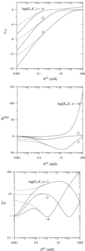
Before the evaluation of the settling velocity of the charge-regulating spheres and the sedimentation potential in the sus-pension from Eqs. [22] and [25], respectively, it is necessary to know how the equilibrium surface potentialζ, equilibrium surface charge densityσ(eq), and charge regulation coefficient L depend on the bulk electrolyte concentration n∞, surface reac-tion equilibrium constants K+ and K− (defined by Eq. [A2]), and particle volume fraction ϕ. To perform a typical calcula-tion using Eqs. [15], [A4], and [A8], we make continuous phase
an aqueous 1 : 1 electrolyte solution with relative permittivity εr = 78.54, the particle radius a = 50 nm, the ionogenic sur-face group density NS= 1 × 10¹⁸site/m2, and the system tem-perature T = 298 K. The numerical results of the dimensionless equilibrium surface potential ¯ζ, equilibrium surface-charge den-sity ¯σ(eq), and charge regulation parameter La calculated as func-tions of the variables n∞, K+K−, K−/K+, andϕ are plotted in Figs. 2 and 3. The value of K+K−is fixed at 10−4M2in Fig. 2 and the value of K−/K+is specified at 10−6in Fig. 3. It can be seen that the point of zero charge is given by n∞= (K+K−)1/2. If n∞< (K+K−)1/2, the values ofζ and σ(eq)are negative; the magnitude ofζ decreases monotonically with an increase in n∞ for an otherwise specified condition, whileσ(eq)has a maximal magnitude at some values of n∞. If n∞> (K+K−)1/2,ζ and
σ(eq)are positive and both increase with an increase in n∞until the value of n∞ is very high. The magnitudes ofζ and σ(eq) increase (so does the value of La) as K−/K+increases, because the concentration of the unionized surface group A B decreases with K−/K+, as inferred from Eq. [A2]. When the value of
K+K− increases, the concentration of negatively charged sur-face groups AZ−will increase or that of the positively charged surface group A B2Z+will decrease according to Eq. [A2]; thus, the particles become more negatively charged or less positively charged. The magnitude ofζ increases, while the magnitudes of σ(eq) and La decrease, as the volume fractionϕ increases, but these dependencies become negligible when the value of n∞or
K−/K+is relatively high.
For the limiting case of an infinitely dilute suspension of charged spheres (ϕ = 0), the dimensionless coefficients in Eqs. [22] and [25] for the sedimentation velocity and sedimen-tation potential reduce to
H = 1
12{e 2κa[5E
6(κa)−3E4(κa)]2−8eκa[E5(κa)− E3(κa)]
+ e2κa[7E
8(2κa) − 3E4(2κa) − 4E3(2κa)]}, [28]
E∗ζ = 1 − eκa[5E7(κa) − 2E5(κa)], [29]
E∗∗ζ = 0, [30] where En is a function defined by
En(x)=
Z ∞
1
t−ne−xtdt. [31] It is interesting that these reduced results, which are the same as the formulas for H and Eζ∗ obtained by Ohshima et al. (7) for a single dielectric sphere in an unbounded electrolyte, do not depend on the charge regulation parameter La. However, it is understood that the value ofζ in Eqs. [22] and [25] for a charge-regulating sphere is dependent on the regulation characteristics of the particle and ambient electrolyte solution.
The numerical results of the dimensionless coefficient H in Eqs. [22] and [23] for the sedimentation velocity of charged spheres in electrolyte solutions calculated as a function of
FIG. 2. Plots of the dimensionless equilibrium surface potential ¯ζ, equilib-rium surface-charge density ¯σ(eq), and charge regulation parameter La versus the bulk concentration n∞of an aqueous 1 : 1 electrolyte solution under the con-ditions a= 50 nm, NS= 1 × 10¹⁸site/m2, and K+K−= 10−4M2. The solid and
dashed curves represent the cases of the volume fractionϕ equal to 0.2 and 0, respectively.
FIG. 3. Plots of the dimensionless equilibrium surface potential ¯ζ , equilib-rium surface-charge density ¯σ(eq), and charge regulation parameter La versus
the bulk concentration n∞ of an aqueous 1 : 1 electrolyte solution under the condition of a= 50 nm, NS= 1 × 10¹⁸site/m2, and K−/K+= 10−6. The solid and dashed curves represent the cases of volume fractionϕ equal to 0.2 and 0, respectively.
FIG. 4. Plots of the dimensionless coefficient H in Eq. [22] for sediment-ing spheres versus parametersκa and ϕ. The solid, dotted, and dashed curves represent the cases of the charge regulation parameter La equal to 0, 5, and∞, respectively.
the parameters κa, La, and ϕ are plotted in Fig. 4 for the Happel cell model. The calculations are presented up to ϕ = 0.74, which corresponds to the maximum attainable volume fraction for a swarm of identical spheres (24). The fact that H is always positive demonstrates that the presence of the surface charges reduces the sedimentation rate for any volume fraction of particles in the suspension. It can be seen that the effect of the surface charges on the sedimentation rate decreases gently and monotonically with an increase in the charge regulation pa-rameter La for given values ofκa and ϕ. This effect becomes independent of La in the case of very dilute suspensions and
for very large and very small values of κa. For fixed values of La andϕ, the coefficient H has a maximum at some finite value of κa and vanishes in the limits κa → 0 and κa → ∞. The location of the maximum shifts to greaterκa as La or ϕ increases. For specified values ofκa and La in a broad range,
H is not a monotonic function ofϕ and has a maximal value.
The location of this maximum shifts to greaterϕ as κa increases or La decreases.
The first-order coefficient Eζ∗in Eq. [25] for the sedimentation potential in suspensions of identical charged spheres is not a function of the charge regulation parameter La, and its relation
FIG. 5. Plots of the dimensionless coefficient Eζ∗∗in Eq. [25] for the sed-imentation potential in a suspension of identical spheres versus parametersκa andϕ. The solid, dotted, and dashed curves represent the cases of the charge regulation parameter La being equal to 0, 5, and∞, respectively.
to the parameters κa and ϕ has already been discussed in a previous article (13; the termϕ−1/3(κa)3 in its Eqs. [52a] and [52b] should be omitted). Figure 5 shows plots of numerical results for the second-order coefficient E∗∗ζ as a function of the parametersκa, La, and ϕ for the Happel model. Analogous to the coefficient H illustrated in Fig. 4, Eζ∗∗is always a positive value, decreases monotonically with an increase in the charge regulation parameter La for fixed values of κa and ϕ, has a maximum at some finite value ofκa for constant values of La andϕ, and may be maximal at a value of ϕ for given values of κa and La. For the limiting casesκa → 0, κa → ∞, or ϕ → 0, the value of Eζ∗∗equals zero.
For conciseness, the numerical results of the dimensionless coefficients H and Eζ∗∗as functions of the parametersκa, La, andϕ for the Kuwabara cell model are not presented here. How-ever, it can be shown that these results are qualitatively similar and quantitatively close to those for the Happel cell model. For a given suspension of identical charge-regulating spheres, the sedimentation velocity and potential for each model can be eval-uated as functions of the regulation characteristics of the suspen-sion (such as n∞, K+, K−, NS, a, and ϕ, etc.) from Eqs. [22] and [25] incorporating Eqs. [15], [A4], and [A8]. These func-tions are quite complicated for most situafunc-tions, and cannot be predicted systematically by simple general rules.
7. SUMMARY
In this work, the steady-state sedimentation phenomena in ho-mogeneous suspensions of identical charge-regulating spheres in electrolyte solutions with arbitrary values ofκa, La, and ϕ are analyzed by employing the Happel and Kuwabara cell mod-els. Solving the linearized electrokinetic equations applicable to the system of a sphere in a unit cell by a regular perturbation method, we have obtained the ion concentration (or electrochem-ical potential energy) distributions, the electric potential profile, and the fluid flow field through the use of a linearized charge regulation model. The requirement that the total force exerted on the particle be zero leads to an explicit formula, Eq. [22], for the settling velocity of the charged spheres. The correction for the effect of the particle charges to the settling velocity begins at the second order,ζ2. Numerical results indicate that this ef-fect has a maximum at some finite values ofκa and disappears when κa approaches zero and infinity. Another explicit for-mula, Eq. [25], for the sedimentation potential is also derived to orderζ2by letting the net electric current in the suspension be zero. It is found that the effects of charge regulation at the par-ticle surface on the sedimentation velocity and potential occur in the leading order ofζ, which is dependent on the regulation characteristics of the suspension.
Equations [22]–[27] are obtained on the basis of the Debye– Huckel approximation for the equilibrium potential distribution around the charged sphere in a unit cell. The reduced formula of Eq. [23] for the sedimentation velocity of a charged sphere with low zeta potential in an unbounded electrolyte solution, Eq. [28],
was shown to give an excellent approximation for the case of reasonably high zeta potential (with an error less than 0.1% for
|ζ |e/kT ≤ 2 in a KCl solution) (7). Therefore, our results might
be used tentatively for the situation of reasonably high electric potentials.
APPENDIX A
Model for a Charge-Regulating Surface
Following the previous studies (15, 16, 22), we consider a general model for the charge-regulating surface which develops surface charges via association/dissociation equilibrium of iono-genic surface groups. The surface reactions may by expressed as
A B2Z+⇔ AB + BZ+, [A1a]
A B⇔ AZ−+ BZ+, [A1b] where A B represents the associable/dissociable functional group on the surface, BZ+denotes the ion that determines the sta-tus of charges on the surface groups (the potential-determining ion), and the positive integer Z is the valence of ionization. For the case of an amphoteric surface, BZ+is usually the hydrogen ion H+. The equilibrium constants for the reactions in Eq. [A1] are given by K+ = [AB][BZ+]S ±£ A B2Z+¤, [A2a] K− = [AZ−][BZ+]S/[AB], [A2b] where [BZ+]
Sis the concentration of BZ+next to the surface. The surface dissociation constants K+ and K− are taken to be functions of temperature only.
For NSionizable surface groups per unit area, the net surface charge density is σ = ZeNS £ A B2Z+¤− [AZ−] [ A B]+£A B2Z+¤+ [AZ−] = ZeNS [BZ+]2S− K+K− K+[BZ+] S+ [BZ+]2S+ K+K− . [A3]
By the substitution of the Boltzmann distribution for the equi-librium concentration of BZ+and the utilization of the concept of electrochemical potential energy (7), Eq. [A3] forσ can be expressed in terms of the surface potentialψSas
σ = ZeNS δ sinh{[Ze(ψN− ψS)+ δµS]/kT } 1+ δ cosh{[Ze(ψN− ψS)+ δµS]/kT } , [A4] where δ = 2(K−/K+)1/2, [A5] ψN= kT Z eln n∞ (K+K−)1/2, [A6]
δµSis the deviation in electrochemical potential of BZ+next to the surface from the equilibrium state defined by Eq. [6], and
n∞is the concentration of BZ+in the bulk solutions, where the equilibrium potential is set equal to zero. Equation [A6] is the Nernst equation relating the Nernst potentialψNto the isoelec-tric point [with n∞= (K+K−)1/2]. It can be seen from Eq. [A4], which acts as an equation of the electric state of the surface, that the sign ofσ is opposite that of ψS− ψNat equilibrium (with
δµS= 0). The equilibrium surface-charge density approaches the saturation values±ZeNSwhen the difference between the equilibrium surface potential and its Nernst value becomes large (e.g., when the value of n∞/(K+K−)1/2approaches zero or in-finity and the value ofψSis finite).
With the relationship betweenσ and ψSgiven by Eq. [A4], the charge regulation capacitance of the surface at equilibrium can be written as − Ã dσ dψS ! ψS=ζ = ε 4πL, [A7]
whereζ is the value of ψSat equilibrium and
L= 4π Z 2e2N Sδ © δ + cosh£Z e¡ψN(eq)− ζ¢±kT¤ª εkT©1+ δ cosh£Z e¡ψN(eq)− ζ¢±kT¤ª2 . [A8]
The reciprocal of the positive quantity L can be regarded as the characteristic length controlling the charge regulation condition at the surface. The limiting values of L= 0 and L → ∞ corre-spond to the cases of constant surface-charge density and con-stant surface potential, respectively. Note that L is small when the difference between the equilibrium surface potential and its Nernst value is large.
APPENDIX B
Definitions of Some Functions in Section 3
For conciseness the definitions of some functions in Section 3 are listed here. In Eq. [17],
Fir(r )= Ci 1+ Ci 2 µ a r ¶ + Ci 3 µ a r ¶3 + Ci 4 µ r a ¶2 + δi 2 εκ 2 24πη × · G1(r )− 1 rG2(r )+ 1 5r3G4(r )− r2 5G−1(r ) ¸ , [B1a] Fiθ(r )= −Ci 1− Ci 2 2 µ a r ¶ +Ci 3 2 µ a r ¶3 − 2Ci 4 µ r a ¶2 + δi 2 εκ2 12πη · −1 2G1(r )+ 1 4rG2(r ) + 1 20r3G4(r )+ r2 5G−1(r ) ¸ , [B1b] Fpi(r )= Ci 2 µ a r ¶2 + 10Ci 4 µ r a ¶ + δi 2 εκ2a 12πη × · − 1 2r2G2(r )− rG−1(r ) ¸ , [B1c]
for i = 0 and 2. In the above equations, the functions Gn(r ) are defined by Eq. [21],δi jis the Kronecker delta which equals unity if i = j but vanishes otherwise,
Ci 1 = − 1 2 £¡ 2+ 3ϕ5/3¢Ai+ 5ϕBi ¤ ω, [B2a] Ci 2 = 1 2 £¡ 3+ 2ϕ5/3¢Ai+ 5ϕ2/3Bi ¤ ω, [B2b] Ci 3 = − 1 2 £ Ai+ ¡ 3ϕ2/3− 2ϕ¢Bi ¤ ω, [B2c] Ci 4 = 1 2 £ ϕ5/3A i− ¡ 2ϕ2/3− 3ϕ¢Bi ¤ ω [B2d]
for the Happel model, and
Ci 1 = − 1 2 £ (2+ ϕ)A0i+¡2− 5ϕ + 3ϕ5/3¢Bi0¤ω0, [B3a] Ci 2 = 1 2 £ 3 A0i+¡3− 5ϕ2/3+ 2ϕ5/3¢Bi0¤ω0, [B3b] Ci 3 = − 1 10 £ (5− 2ϕ)A0i+ 5¡1− 3ϕ2/3+ 2ϕ¢Bi0¤ω0, [B3c] Ci 4 = 1 10 £ 3ϕ A0i+ 5¡2ϕ2/3− 3ϕ + ϕ5/3¢Bi0¤ω0 [B3d] for the Kuwabara model, where
Ai = δi 0+ δi 2 εκ2 24πη · G1(b)− 1 bG2(b) ¸ , [B4a] Bi = δi 2 εκ2 120πη · 1 b3G4(b)− b 2G −1(b) ¸ , [B4b] A0i = δi 0+ δi 2 εκ2 24πη · G1(b)− 1 bG2(b) + 1 5b3G4(b)− b2 5G−1(b) ¸ , [B5a] Bi0= δi 2 εκ2 120πη · −1 bG2(b)+ b 2G −1(b) ¸ , [B5b] ω = µ 1−3 2ϕ 1/3+3 2ϕ 5/3− ϕ2 ¶−1 , [B6a] ω0=µ1−9 5ϕ 1/3+ ϕ −1 5ϕ 2 ¶−1 . [B6b]
In Eqs. [18] and [19], F1±(r )= ± 1 6D±(1− ϕ)r2 ½ a3Aµ(a, b) + 2ϕBµ(a, b) + 2r3 · ϕ Aµ(a, b) + 2 b3Bµ(a, b) ¸ + 2(1 − ϕ)[Bµ(a, r) + r3Aµ(r, b)] ¾ , [B7] Fψ1(r )= e2κa[2+ La + κa(κa − La − 2)]J × {Aψ(a, b)e2κb[κb(κb − 2) + 2] + Bψ(a, b)[κb(κb + 2) + 2]} µ κr + 1 r2 ¶ e−κr
+ [κb(κb + 2) + 2]J{Aψ(a, b)e2κa[κa(κa − La − 2) + La + 2] + Bψ(a, b)[κa(κa + La + 2) + La + 2]} µκr − 1 r2 ¶ eκr + µ κr + 1 r2 ¶ e−κrBψ(a, r) + µ κr − 1 r2 ¶ eκrAψ(r, b), [B8] where Aµ(x, y) = Z y x F0r(r ) dψeq1 dr dr, [B9a] Bµ(x, y) = Z y x r3F0r(r ) dψeq1 dr dr, [B9b] Aψ(x, y) = Z y x κr + 1 4κ e −κr[F 1+(r )− F1−(r )] dr, [B10a] Bψ(x, y) = Z y x κr − 1 4κ e κr[F 1+(r )− F1−(r )] dr, [B10b] J = {e2κb[κa(κa + La + 2) + La + 2][κb(κb − 2) + 2] − e2κa[κa(κa − La − 2) + La + 2][κb(κb + 2) + 2]}−1. [B11] In the limit La→ ∞, Eq. [B8] reduces to
Fψ1(r )= −e2κa(κa − 1)J∞{Aψ(a, b)e2κb[κb(κb − 2) + 2]
+ Bψ(a, b)[κb(κb + 2) + 2]} µ κr + 1 r2 ¶ e−κr
+ [κb(κb + 2) + 2]J∞[−Aψ(a, b)e2κa(κa − 1)
+ Bψ(a, b)(κa + 1)] µ κr − 1 r2 ¶ eκr+ µ κr + 1 r2 ¶ e−κr × Bψ(a, r) + µκr − 1 r2 ¶ eκrAψ(r, b), [B12] where J∞= {(κa + 1)[κb(κb − 2) + 2]e2κb
+ (κa − 1)[κb(κb + 2) + 2]e2κa}−1. [B13] ACKNOWLEDGMENT
This research was partially supported by the National Science Council of the Republic of China.
REFERENCES
1. Booth, F., J. Chem. Phys. 22, 1956 (1954).
2. Dukhin, S. S., and Derjaguin, B. V., in “Surface and Colloid Science” (E. Matijevic, Ed.), Vol. 7. Wiley, New York, 1974.
3. Saville, D. A., Adv. Colloid Interface Sci. 16, 267 (1982). 4. Stigter, D., J. Phys. Chem. 84, 2758 (1980).
5. Wiersema, P. H., Leob, A. L., and Overbeek, J. Th. G., J. Colloid Interface
Sci. 22, 78 (1966).
6. de Groot, S. R., Mazur, P., and Overbeek, J. Th. G., J. Chem. Phys. 20, 1825 (1952).
7. Ohshima, H., Healy, T. W., White, L. R., and O’Brien, R. W., J. Chem. Soc.,
Faraday Trans. 2 80, 1299 (1984).
8. Keh, H. J., and Liu, Y. C., J. Colloid Interface Sci. 195, 169 (1997).
9. Happel, J., AIChE J. 4, 197 (1958).
10. Kuwabara, S., J. Phys. Soc. Jpn. 14, 527 (1959).
11. Levine, S., Neale, G., and Epstein, N., J. Colloid Interface Sci. 57, 424 (1976).
12. Ohshima, H., J. Colloid Interface Sci. 208, 295 (1998).
13. Keh, H. J., and Ding, J. M., J. Colloid Interface Sci. 227, 540 (2000). 14. Ninham, B. W., and Parsegian, V. A., J. Theor. Biol. 31, 405 (1971). 15. Chan, D., Perram, J. W., White, L. R., and Healy, T. W., J. Chem. Soc.
Faraday Trans. 1 71, 1046 (1975).
16. Chan, D., Healy, T. W., White, L. R., J. Chem. Soc. Faraday Trans. 1 72, 2844 (1976).
17. Prieve, D. C., and Ruckenstein, E., J Theor. Biol. 56, 205 (1976). 18. Van Riemsdijk, W. H., Bolt, G. H., Koopal, L. K., and Blaakmeer, J.,
J. Colloid Interface Sci. 109, 219 (1986).
19. Krozel, J. W., and Saville, D. A., J. Colloid Interface Sci. 150, 365 (1992).
20. Carnie, S. L., and Chan, D. Y. C., J. Colloid Interface Sci. 161, 260 (1993).
21. Pujar, N. S., and Zydney, A. L., J. Colloid Interface Sci. 192, 338 (1997).
22. Hsu, J., and Liu, B., Langmuir 15, 5219 (1999).
23. Happel, J., and Brenner, H., “Low Reynolds Number Hydrodynamics.” Nijhoff, Dordrecht, 1983.
![FIG. 5. Plots of the dimensionless coefficient E ζ ∗∗ in Eq. [25] for the sed- sed-imentation potential in a suspension of identical spheres versus parameters κa and ϕ](https://thumb-ap.123doks.com/thumbv2/9libinfo/8844166.239921/8.918.481.879.328.1093/dimensionless-coefficient-imentation-potential-suspension-identical-spheres-parameters.webp)
