a note on 15/8 & 3/2-approximation algorithms for the MRCT problem

A note on 15/8 & 3/2-approximation algorithms for

the MRCT problem

Bang Ye Wu Kun–Mao Chao

March 18, 2004

1

Approximating by a General Star

1.1 Separators and general stars

A key point to the 2-approximation in our previous note is the existence of the centroid, which separates a tree into sufficiently small components. To generalize the idea, we define the separator of a tree in Definition 1.

Definition 1 : Let T be a spanning tree of G and S be a connected subgraph of T . A branch of S is a connected component of the subgraph that results by removing S from T .

Definition 2: Let δ ≤ 1/2. A connected subgraph S is a δ-separator of T if |B| ≤ δ|V (T )| for every branch B of S.

A separator S is minimal if any proper subgraph of S is not a δ-separator of T .

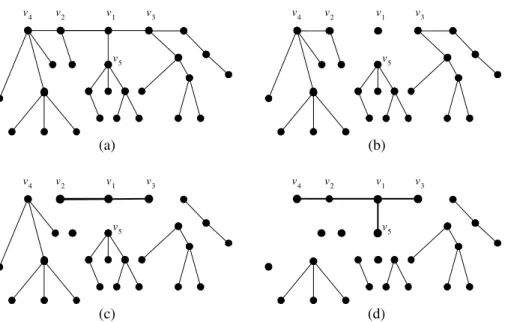
Example 1: The tree in Figure 1(a) has 26 vertices in which v1is a centroid. The vertex v1 is a minimal 1/2-separator. As shown in (b), each branch contains no more than 13 vertices. But v₁, or even the edge (v₁, v₂), is not a 1/3-separator because there exists a subtree whose number of vertices is nine, which is greater than 26/3. The path between v2 and v3 is a minimal 1/3-separator (Frame (c)), and the subgraph that consists of v₁, v₂, v₃, v₄,

and v5 is a minimal 1/4-separator (Frame (d)).

The δ-separator can be thought of as a generalization of the centroid of a tree. Obviously, a centroid is a 1/2-separator which contains only one node. Intuitively, a separator is like a routing center of the tree. Starting from

v 1 v 2 v3 v 4 v 5 v 1 v 2 v3 v 4 v 5 v 1 v 2 v3 v 4 v 5 v 1 v 2 v3 v 4 v 5 (a) (b) (d) (c)

Figure 1: An example of a minimal separator of a tree.

any node, there are sufficiently many nodes which can only be reached after reaching the separator. For two vertices i and j in different components separated by S, the path between them can be divided into three subpaths: from i to S, a path in S, and from S to j. Since each component contains no more than δn vertices, the distance dT(i, S) will be counted at least

2(1 − δ)n times as we compute the routing cost of T . For each edge e in S, since there are at least δn vertices on either side of the edge, by Fact ??, the routing load on e is at least 2δ(1 − δ)n2_{. Some notations are given below} and illustrated in Figure 2.

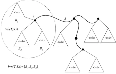
Definition 3 : Let T be a spanning tree of G and S be a connected subgraph of T . Let u be a vertex in S. The set of branches of S connected to u by an edge of T is denoted by brn(T, S, u), while brn(T, S) is for the set of all branches of S. The set of vertices in the branches connected to u is denoted by V B(T, S, u) = {u} ∪ {v|v ∈ B ∈ brn(T, S, u)}.

The next fact directly follows the definitions.

Fact 1: Let S be a minimal δ-separator of T . If v is a leaf of S, then

<=kn <=kn <=kn <=kn <=kn <=kn <=kn <=kn i S brn(T,S,i)={B₁,B₂,B₃} B₁ B₂ B₃ VB(T,S,i)

Figure 2: A δ-separator and branches of a tree. The bold line is the separator

S and each triangle is a branch of S.

A star is a tree with only one internal vertex (center). We define a

general star as follows.

Definition 4: Let R be a tree contained in the underlying graph G. A spanning tree T is a general star with core R if each vertex is connected to

R by a shortest path.

For an extreme example, a shortest-paths tree is a general star whose core contains only one vertex. By star(R), we denote the set of all general stars with core R. The intuition of using general stars to approximate an MRCT is described as follows: Assume S is a δ-separator of an optimal tree T . The separator breaks the tree into sufficiently small components (branches). The routing cost of T is the sum of the distances of the n(n − 1) pairs of vertices. If we divide the routing cost into two terms, the total distance of vertices in different branches and the total distance of vertices in a same branch, then the inter-branch distance is the larger fraction of the total routing cost. Furthermore, the fraction gets larger and larger when a smaller δ is chosen. If we construct a general star with core S, the routing cost will be very close to the optimal.

Given a core, to construct a general star is just to find a shortest-paths forest, which can be done in O(n log n + m) time. However, it can be done

more efficiently if the all-pairs shortest paths are given.

Lemma 1: Let G be a graph, and let S be a tree contained in G. A spanning tree T ∈ star(S) can be found in O(n) time if a shortest path

SPG(v, S) is given for every v ∈ V (G).

Proof: A constructive proof is given below. Starting from T = S, we show a procedure which inserts all other vertices into T one by one. At each iteration, the following equality is kept:

dT(v, S) = dG(v, S) ∀v ∈ V (T ). (1)

It is easy to see that (1) is true initially. Consider the step of inserting a ver-tex. Let SP_G(v, S) = (v = v₁, v₂, ..., v_k∈ S) be a shortest path from v to S,

and let vjbe the first vertex which is already in T . Set T ← T ∪(v1, v2, ..., vj).

Since (v1, v2, ..., vk) is a shortest path from v to S, (va, va+1, ..., vj) is also a

shortest path from v_a to v_j for any a = 1, . . . j, and (1) is true. It is easy to see that the time complexity is O(n), if a shortest path from v to S is given for every v ∈ V .

Let S be a connected subgraph of a spanning tree T . The path between two vertices v and u in different branches can be divided into three subpaths: the path from v to S, the path contained in S, and the path from u to S. For convenience, we define dS_T(u, v) = w(SPT(u, v) ∩ S). Obviously

dT(u, v) ≤ dT(v, S) + dST(u, v) + dT(u, S), (2)

and the equality holds if v and u are in different branches. Summing up (2) for all pairs of vertices, we have

C(T ) ≤ 2nX v∈V dT(v, S) + X u,v∈V dS_T(u, v).

By the definition of routing load,

X

u,v∈V

dS_T(u, v) = X

e∈E(S)

l(T, e)w(e).

Suppose that T is a general star with core S. We can establish an upper bound of the routing cost by observing that dT(v, S) = dG(v, S) for any

vertex v and l(T, e) ≤ n₂2 for any edge e (Fact ??).

Lemma 2: Let G be a graph and S be a tree contained in G. If T ∈ star(S), C(T ) ≤ 2nP_{v∈V (G)}dG(v, S) + (n2/2)w(S).

Now we establish a lower bound of the minimum routing cost. Let S be a minimal δ-separator of a spanning tree T and X denote the set of the ordered pairs of the vertices not in a same branch of S. For any vertex pair (u, v) ∈ X ,

d_T(u, v) = d_T(u, S) + dS_T(u, v) + d_T(v, S). (3) Summing up (3) for all pairs in X , we have a lower bound of C(T ).

C(T ) ≥ X (u,v)∈X d_T(u, v) = X (u,v)∈X (d_T(u, S) + d_T(v, S)) + X (u,v)∈X dS_T(u, v). (4)

Since S is a δ-separator, there are at least (1 − δ)n vertices not in the same branch of any vertex v, and we have

X (u,v)∈X (dT(u, S) + dT(v, S)) ≥ 2(1 − δ)n X v∈V dT(v, S). (5) Since dS

T(u, v) = 0 if v and u are in the same branch,

X (u,v)∈X dS_T(u, v) =X v X u dS_T(u, v).

By definition, this is the total routing cost on the edges of S. Rewriting this in terms of routing loads, we have

X v X u dS_T(u, v) = X e∈E(S) l(T, e)w(e). (6)

Substituting (5) and (6) in (4), we have

C(T ) ≥ 2(1 − δ)nX v∈V dT(v, S) + X e∈E(S) l(T, e)w(e). (7)

Since S is a minimal δ-separator, for any edge of S there are at least δn vertices on either side of the edge. Therefore, l(T, e) ≥ 2δ(1 − δ)n2 _{for any}

e ∈ E(S). Consequently, X e∈E(S) l(T, e)w(e) ≥ 2δ(1 − δ)n2 X e∈E(S) w(e) = 2δ(1 − δ)n2w(S). (8)

Combining (7) and (8), we obtain

C(T ) ≥ 2(1 − δ)nX

v∈V

d_T(v, S) + 2δ(1 − δ)n2w(S). (9)

Lemma 3: If S is a minimal δ-separator ofT , thenb C(T ) ≥ 2(1 − δ)nb X

v∈V

d_Tb(v, S) + 2δ(1 − δ)n2w(S).

1.2 A 15/8-approximation algorithm

In our previous note, a 1/2-separator is used to derive a 2-approximation algorithm. The idea is now generalized to show that a better approximation ratio can be obtained by using a 1/3-separator. The following lemma shows the existence of a 1/3-separator. Note that a path may contain only one vertex.

Lemma 4 : For any tree T , there is a path P ⊂ T , such that P is a 1/3-separator of T .

Proof: Let n be the number of vertices of T and r be a centroid of T . There are at most 2 branches of r, in which the number of vertices exceed

n/3. If there is no such branch, then r is itself a 1/3-separator. Let A be a

branch of r with |V (A)| > n/3. Since A itself is a tree with no more than

n/2 vertices, a centroid ra of A is a 1/2-separator of A, and each branch of

ra contains no more than n/4 vertices of A. If there is another branch B of

r such that |V (B)| > n/3, a centroid r_b of B can be found such that each branch of rb contains no more than n/4 vertices of B. Consider the path

P = SPT(ra, r) ∪ SPT(r, rb). Since each branch of P contains no more than

n/3 vertices, P is a 1/3-separator of T . Note that if B does not exist, then SPT(ra, r) is a 1/3-separator.

In the following paragraphs, a path separator of a tree T is a path and meanwhile a minimal 1/3-separator of T . Substituting δ = 1/3 in Lemma 3, we obtain a lower bound of the minimum routing cost.

Corollary 5: If P is a path separator ofT , thenb

C(T ) ≥b 4n 3 X v∈V d_Tb(v, P ) +4n2 9 w(P ).

Lemma 6: There exist r1, r2 ∈ V such that if R = SPG(r1, r2) and T ∈ star(R), C(T ) ≤ (15/8)C(T ).b

Proof: Let P be a path separator of T with endpoints rb 1 and r2. Since

T is a general star with core R, by Lemma 2, C(T ) ≤ 2n X

v∈V (G)

d_G(v, R) + n2

2 w(R). (10)

Let S = V B(T , P, rb ₁)∪V B(T , P, rb ₂) denote the set of vertices in the branches incident to the two endpoints of P . For any v ∈ S,

d_G(v, R) ≤ min{d_G(v, r₁), d_G(v, r₂)} ≤ d_Tb(v, P ). For v /∈ S, dG(v, R) ≤ min{dG(v, r1), dG(v, r2)} ≤ (d_G(v, r₁) + d_G(v, r₂)) /2 ≤ d_Tb(v, P ) + w(P )/2. Then, by Fact 1, |S| ≥ 2n₃ , and therefore

X v∈V dG(v, R) ≤ X v∈V d_Tb(v, P ) + (n/6)w(P ). (11)

Substituting this in (10) and recalling that w(R) ≤ w(P ) since R is a shortest path between r1 and r2, we have

C(T ) ≤ 2nX

v∈V

d_Tb(v, P ) + (5n2/6)w(P ). (12)

Comparing with the lower bound in Corollary 5, we obtain

C(T ) ≤ max{3/2, 15/8}C(T ) = (15/8)C(b T ).b

By Lemma 6 we can have a 15/8-approximation algorithm for the MRCT problem. For every r1 and r2 in V , we construct a shortest path R =

SPG(r1, r2) and a general star T ∈ star(R) including the degenerated cases

r1 = r2. The one with the minimum routing cost must be a 15/8-approximation of the MRCT. All-pairs shortest paths can be found in O(n3_{) time. A direct} method takes O(n log n + m) time for each pair r1 and r2, and therefore

O(n3log n + n2m) time in total. In the next lemma, it is shown that this

Lemma 7: Let G = (V, E, w). There is an algorithm which constructs a general star T ∈ star(SPG(r1, r2)) for every vertex pair r1 and r2 in O(n3) time.

Proof: For any r ∈ V , if a general star T ∈ star(SPG(r, v)) for each v ∈ V

can be constructed with total time complexity O(n2_{), then all the stars can} be constructed in O(n3) time by applying the algorithm n times for each

r ∈ V . By Lemma 1, a star T ∈ star(SPG(r, v)) can be constructed in O(n)

time if, for every u ∈ V , a shortest path from u to SP_G(r, v) is given. Define

A(u, v) = dG(u, SPG(r, v)) and B(u, v) to be the vertex k ∈ SPG(r, v) such

that SPG(u, k) = SPG(u, SPG(r, v)). Since the all-pairs shortest paths can

be constructed in O(n2_{log n + mn) time at the preprocessing stage, we need} to compute A(u, v), as well as B(u, v), in O(n2) time for all u, v ∈ V .

First, construct a shortest-paths tree S rooted at r. Let parent(v) denote the parent of v in S. It is not hard to see that

A(u, v) = min{A(parent(v), u), dG(u, v)}

for u, v ∈ V −{r}, and A(r, u) = d_G(r, u). Therefore by a top-down traversal of S, we can compute A(u, v) and B(u, v) for all u, v ∈ V in O(n2_{) time.}

The next theorem can be derived directly from Lemmas 6 and 7. Theorem 8 : There is a 15/8-approximation algorithm for the MRCT problem with time complexity O(n3_).

1.3 A 3/2-approximation algorithm

Let P be a path separator of an optimal tree. By Lemma 2, if X ∈ star(P ), then

C(X) ≤ 2nX

v∈V

d_G(v, P ) + (n2/2)w(P ).

Since dG(v, P ) ≤ d_Tb(v, P ) for any v, it can be shown that X is a

3/2-approximation solution by Corollary 5. However, it costs exponential time to try all possible paths. In the following we show that a 3/2-approximation solution can be found if, in addition to the two endpoints of P , we know a centroid of an optimal tree.

Let P = (p1, p2, ..., pk) be a path separator of T , Vb i = V B(T, P, pi), and

ni= |Vi| for 1 ≤ i ≤ k. It is easy to see that a centroid must be in V (P ). Let

pqbe a centroid ofT . Construct R = SPb G(p1, pq) ∪ SPG(pq, pk). We assume

that R has no cycle. Otherwise, we arbitrarily remove edges to break the cycles. Obviously w(R) ≤ w(P ). Let T ∈ star(R). The next lemma shows the approximation ratio.

Lemma 9: C(T ) ≤ (3/2)C(T ).b

Proof: First, for any v ∈ V1∪ Vq∪ Vk,

dG(v, R) ≤ min{dG(v, p1), dG(v, pq), dG(v, pk)} ≤ d_Tb(v, P ). For v ∈S_1<i<qV_i, dG(v, R) ≤ min{dG(v, p1), dG(v, pq)} ≤ (dG(v, p1) + dG(v, pq)) /2 ≤ d_Tb(v, P ) + d_Tb(p1, pq)/2.

Similarly, for v ∈S_q<i<kVi,

dG(v, S) ≤ d_Tb(v, P ) + d_Tb(pq, pk)/2.

By Fact 1 and the property of a centroid, we have P 1<i<q n_i ≤ n/6 and P q<i<k ni ≤ n/6. Thus, X v∈V dG(v, R) ≤ X v∈V d_Tb(v, P ) + (n/12)w(P ).

By Lemma 2 and Corollary 5,

C(T ) ≤ 2nX v∈V dG(v, R) + (n2/2)w(R) ≤ 2nX v∈V d_Tb(v, P ) + (2n2/3)w(P ) ≤ (3/2)C(T ).b

Theorem 10: There is a 3/2-approximation algorithm with time com-plexity O(n4_{) for the MRCT problem.}

Proof: First, the all-pairs shortest paths can be found in O(n2log n +

mn). For every triple (r1, r0, r2) of vertices, we construct R = SPG(r1, r0) ∪

SPG(r0, r2) and T ∈ star(R) including the degenerated cases ri = rj. By

Lemma 9, at least one of these stars is a 3/2-approximation solution of the MRCT problem, and we can choose the one with the minimum routing

cost. For the time complexity, we show that each star can be constructed in O(n) time. By Lemma 1, a T ∈ star(R) can be constructed in O(n) time if for every v ∈ V , a shortest path from v to R is given. Define

A(i, j, k) = dG(i, SPG(j, k)) and B(i, j, k) to be the vertex in SPG(j, k)

which is closest to i. It is easy to see that A(i, j, k) and B(i, j, k) can be computed in O(n4_{) time.}1 _{For any R = SP}

G(r1, r0) ∪ SPG(r0, r2), since

dG(v, R) = min{A(v, r1, r0), A(v, r0, r2)},

d_G(v, R) as well as the vertex in R closest to v can be computed in total

O(n4) time for all v ∈ V and for all such R at a preprocessing step. Finally, for any spanning tree T , we can compute C(T ) in O(n) time. So the total time complexity is O(n4_).

1_{Remark: It can be computed in O(n}3_{) time by dynamic programming. However the}