On the Reduction of Numerical Dissipation in Central-Upwind Schemes

Central-Upwind Schemes

Alexander Kurganov

_{and Chi-Tien Lin}

Abstract

We study central-upwind schemes for systems of hyperbolic conservation laws, recently introduced in [A. Kurganov, S. Noelle and G. Petrova, SIAM J. Sci. Comput., 23 (2001), pp. 707–740]. Similarly to the staggered central schemes, these schemes are central Godunov-type projection-evolution methods that enjoy the advantages of high resolution, simplicity, universality, and robustness. At the same time, the central-upwind framework allows one to decrease a relatively large amount of numerical dissipation present at the staggered central schemes.

In this paper, we present a modification of the one-dimensional fully- and semi-discrete central-upwind schemes, in which the numerical dissipation is reduced even further. The goal is achieved by a more accurate projection of the evolved quan-tities onto the original grid. In the semi-discrete case, the reduction of dissipation procedure leads to a new, less dissipative numerical flux. We also extend the new semi-discrete scheme to the two-dimensional case via the rigorous, genuinely multi-dimensional derivation.

The new semi-discrete schemes are tested on a number of numerical examples, where one can observe an improved resolution, especially of the contact waves.

1

Introduction

Consider the systems of hyperbolic conservation laws, ∂

∂tu(x, t) + ∇x·f (u(x, t)) = 0, (1.1)

where u(x, t) = (u1(x, t), . . . , uN(x, t))T is an N-dimensional vector and f is a nonlinear

con-vection flux. In the general multidimensional case, u is a vector function of a time variable

t and d-spatial variables x = (x1, . . . , xd) with the corresponding fluxes f = (f1, . . . , fd).

†_{Department of Mathematics, Tulane University, New Orleans, LA 70118; [email protected]} ‡_{Department of Applied Mathematics, Providence University, Shalu, Taiwan 43301; [email protected]}

Such systems arise in many different applications, for instance, in fluid mechanics, geo-physics, meteorology, astrogeo-physics, financial and biological modelling, multi-component flows, groundwater flow, semiconductors, reactive flows, geometric optics, traffic flow, and other areas.

We study numerical methods for system (1.1). In particular, we are interested in Godunov-type finite-volume central schemes, which are simple, robust, and universal Riemann-problem-solver-free methods for general systems of conservation laws. The key idea in their construction is the integration over the shifted control volumes that contain the entire Rie-mann fans. Such a setting allows one to evolve a piecewise polynomial projections of the computed solution to the next time level without (approximately) solving (generalized) Riemann problems, arising at cell interfaces.

The prototype central scheme is the celebrated (staggered) Lax-Friedrichs scheme [4]. This is a very dissipative first-order scheme, which typically cannot provide a satisfac-tory resolution of discontinuities and rarefaction corners unless a very large number of grid points is used. Its higher-order (and also higher resolution) generalization was pro-posed by Nessyahu and Tadmor in [23]. Later the one-dimensional (1-D) second-order Nessyahu-Tadmor scheme was extended to higher orders [21, 18] and to more than one spatial dimensions [1, 2, 8, 19]. Its nonstaggered version was proposed in [7].

The major drawback of staggered central schemes is their relatively large numerical dissipation. This makes them inappropriate for large time integrations, steady-state com-putations, and for the cases where small time steps are enforced, for example, due to the presence of source or diffusion terms on the right-hand side (RHS) of (1.1). They also do not admit a semi-discrete form, which may be particularly advantageous in the latter case (see, e.g., [15, 11, 9]).

In order to eliminate the aforementioned disadvantages, a new class of high-resolution central schemes has been recently proposed in [15]. The main idea in the construction of the new central schemes is to utilize the local propagation speeds to obtain a more precise estimate on the width of Riemann fans. The solution is then evolved separately in “nonsmooth” (those that include Riemann fans) and “smooth” control volumes, and the resulting nonuniformly distributed data are projected back onto the original, non-staggered grid. The higher-order extensions of this scheme were proposed in [10, 13], and its genuinely multidimensional generalization was obtained in [13].

The numerical dissipation present at central schemes can be further reduced by utilizing one-sided local propagation speeds. This leads to the so-called central-upwind schemes, re-cently introduced in [12]. This class of schemes enjoys all the major advantages of Riemann-problem-solver-free central schemes — high efficiency, simplicity and universality. At the same time, it has a certain upwind nature (more information on the directions of wave prop-agation is used since the control volumes over the Riemann fans are no longer symmetric), which leads to a higher resolution.

In this paper, we implement an idea of less dissipative projection step, suggested in the context of partial characteristic decomposition in [14]. This leads to new 1-D fully- and

semi-discrete central-upwind schemes with even smaller numerical viscosity and, as a result, to a further improvement in the resolution of nonsmooth parts of the solution, especially of contact waves. Finally, this approach is generalized for two-dimensional (2-D) systems, and a new multidimensional semi-discrete central-upwind scheme is introduced.

The rest of the paper is organized as follows. In §2, we derive our new fully discrete scheme, while in §3, the new semi-discrete scheme. In §4, we give a 2D construction of fully discrete version. §5, we present some numerical results to show sharper resolution near a contact discontinuities.

2

One-Dimensional Fully-Discrete Scheme

In this section, we describle briefly the construction of the second-order fully-discrete central-upwind scheme in [14] for the 1-D system of hyperbolic conservation laws,

ut+ f (u)x= 0, (2.1)

subject to compactly supported or periodic initial data,

u(x, 0) = u0(x). (2.2)

The scheme is based on the integration of (2.1) over the control volumes, and consists of three consecutive steps — reconstruction, evolution, and projection.

For simplicity, we consider only uniform grids, xα := α∆x. We also assume that at

the current time level, t = tn_{, the computed cell averages of the solution, ¯u}n

j, are available.

Then, the evolution of the computed solution to the next time level, t = tn+1_{, can be}

presented as follows. Step 1: Reconstruction

Using the computed cell averages, {¯un

j}, we reconstruct the second-order piecewise linear

interpolant: e u(x, tn) = X j [¯un_j + sn_j(x − xj)]

χ

j denotes the numerical slope and

χ

cell, (x_j−1

2, xj+ 1

2). Such an interpolant will be second-order accurate provided every slope

sn

j is (at least) first-order approximation of the spatial derivative ux(xj, tn). To avoid

oscillations that may appear at cell interfaces {x_j+1

2}, a nonlinear limiter should be used in

the evaluation of the slopes. A typical example is the minmod limiter. For choice of other nonlinear limiters, consult [17, 23, 26, 6, 20] and the reference therein.

t tn+1 tn x x j xj+1 x j−1 x j−1/2,l xj−1/2,r xj+1/2,l xj+1/2,r x j−1/2 xj+1/2 wn+1 j−1/2 w n+1 j+1/2 wn+1 j

Figure 2.1: Rectangular control volumes in the original central-upwind scheme in [12]. Step 2: Evolution

We first note that the possible discontinuity at the interface points {x_j+1

2} propagate at

only finite speeds. Upper bounds on the right- and left-sided local speeds can be computed by a+_j+1 2 :=_ω∈C(umax− j+ 1₂,u + j+ 1₂) n λN(A(ω)) , 0 o ≥ 0, a−_j+1 2 :=_ω∈C(umin− j+ 1₂,u + j+ 1₂) n λ1(A(ω)) , 0 o ≤ 0, (2.4)

respectively. Here, λ1 < λ2 < . . . < λN are the N eigenvalues of the Jacobian A := ∂f_∂u, and

C(u−

j+1₂, u

+

j+1₂) is the Riemann admissible curve in the phase space that connects the left,

u−

j+1 2

, and the right, u+

j+1 2 , states, u− j+1₂ :=_x→xlim j+ 1₂− e u(x, tn_{), u}+ j+1₂ :=_x→xlim j+ 1₂+ e u(x, tn_{). (2.5)}

Next, we split the strip S = X ×[tn_{, t}n+1_{], where X is the spatial computational domain,}

into nonsmooth areas, [x_j+1

2,l, xj+ 1 2,r]×[t

n_{, t}n+1_{] and smooth areas, [x}

j−1₂,r, xj+1₂,l]×[tn, tn+1]. Here, x_j+1 2,l := xj+ 1 2 + a − j+1₂∆t, xj+12,r := xj+ 1 2 + a + j+1₂∆t. See Figure 2.1.

Finally, we evolve the solution from time level t = tn _{to t}n+1 _{by integrating (2.1) over}

the aforementioned smooth and nonsmooth areas. Using the midpoint quadrature for the temporal integrals under the CFL restriction

∆t max j |a ± j+1 2 | < 1 2∆x, (2.6)

we obtain the following intermediate cell averages at time t = tn+1_{, over nonsmooth area} ¯ wn+1 j+1₂= 1 a+ j+1 2 − a− j+1 2 h un j+1₂,ra + j+1₂ − u n j+1₂,la − j+1₂ − f (u n+1₂ j+1₂,r) + f (u n+1₂ j+1₂,l) i , (2.7)

and, over smooth area ¯ wn+1 j = ¯unj + sn j 2(a + j+1 2 + a− j+1 2 )∆t + ∆t ∆x − (a+_j−1 2 − a − j+1 2)∆t h −f (un+12 j+1 2,l ) + f (un+12 j−1 2,r ) i . (2.8) Here, un_j+1 2,l := ¯u n j + sn j 2(∆x + a − j+1 2∆t); u n j+1₂,r := ¯u n j+1− sn j+1 2 (∆x − a + j+1 2∆t). (2.9)

Finally, the midpoint values, un+12

j+1₂,l := u(xj+12,l, t

n+1_{2) and u}n+12

j+1₂,r := u(xj+12,r, t

n+1_{2), can be}

obtained, using Taylor expansions about the corresponding points (x_j+1

2,l, t n_{) and (x} j+1₂,r, tn), which results in un+12 j+1 2,l = un j+1 2,l− ∆t 2 f (u n j+1 2,l)x, u n+1 2 j+1 2,r = un j+1 2,r− ∆t 2 f (u n j+1 2,r)x. (2.10)

Note that one can avoid the computation of the Jacobians in (2.10) by using a

component-wise evaluation of fx, consult [23] for details.

Step 3: Projection

At the final step, a piecewise linear interpolant, e w(x, tn+1) :=X j ½h ¯ w_j+n+11 2 + s n+1 j+1 2 ³ x − xj+12,l+ xj+12,r 2 ´i

χ

χ

reconstructed from the evolved intermediate cell averages { ¯wn+1

j } and { ¯wn+1_j+1

2

}, is projected

back onto the original grid by averaging it over the intervals [x_j−1

2, xj+ 1

2]. This results in

the new projected cell averages: ¯ un+1_j = λa+_j−1 2w¯ n+1 j−1 2 + h 1 + λ(a−_j+1 2 − a + j+1 2) i ¯ w_jn+1− λa−_j+1 2w¯ n+1 j+1 2 + λ∆t 2 h sn+1 j+1₂a + j+1₂a − j+1₂ − s n+1 j−1₂a + j−1₂a − j−1₂ i . (2.12)

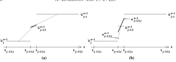
To compute the numerical slopes {sn+1_j+1

2}, one can do this in several different ways. For

example, in [15, 12], the most straightforward component-wise approach has been imple-mented, namely, the slopes have been evaluated by

sn+1_j+1 2 = 2 · minmod à θ w¯ n+1 j+1 2 − ¯w n+1 j x_j+1 2,r− xj− 1 2,r , w¯ n+1 j+1 − ¯wn+1j x_j+3 2,l+ xj+ 1 2,r− xj+ 1 2,l− xj− 1 2,r , θ w¯ n+1 j+1 − ¯wn+1_j+1 2 x_j+3 2,l− xj+ 1 2,l ! , (2.13)

x x x j−1/2,r x j−1/2,r xj+1/2,l xj+1/2,r xj+3/2,l xj+1/2,l xj+1/2,r xj+3/2,l j+1/2 w w j+1/2 n+1 n+1 j+1 n+1 w w j+1 n+1 u_j+1/2,rn+1 j+1/2,l un+1 wn+1_j w_jn+1 (a) (b)

Figure 2.2: Computing the numerical slope sn+1_j+1

2: (a) the approach from [15, 12] with θ = 1

vs. (b) the new, less dissipative approach. see Figure 2.2(a). Here, the distances

x_j+1 2,r− xj− 1 2,r = ∆x + ∆t(a + j+1 2 − a + j−1 2) and xj+ 3 2,l− xj+ 1 2,l = ∆x + ∆t(a − j+3 2 − a − j+1 2)

are of order ∆x for small ∆t, and thus the slopes sn+1

j+1 2

are proportional to ∆w/∆x as ∆t ∼ 0, which may lead to a scheme with a relatively large numerical dissipation. This can be understood if one looks at the last term on the RHS of (2.12). If we assume that ∆x is

fixed, then this term is of order (∆t)2_{, and hence when time-steps are small, the contribution}

of the nonzero slopes in the linear reconstruction (2.11) may become negligible, which would make the projection step to be as diffusive as a first-order projection typically is.

Here, we propose an alternative, less dissipative way of computing sn+1_j+1

2. First, we

approximate the values of the solution at the points x_j+1

2,l and xj+12,r at time level t = t

n+1_,

which will be denoted by un+1

j+1₂,l and u

n+1

j+1₂,r, respectively. Since the solution of the

initial-value problem (2.1),(2.3) is smooth there, we may use the corresponding Taylor expansions, which, similarly to (2.10), give

un+1_j+1 2,l = u n j+1 2,l− ∆tf (u n j+1 2,l)x, u n+1 j+1 2,r = u n j+1 2,r− ∆tf (u n j+1 2,r)x. (2.14)

To prevent the reconstruction (2.11) from being oscillatory, we need to enforce the

mono-tonicity of these values. Namely, if un+1

j+1₂,l (u n+1

j+1₂,r), computed in (2.14), is not between ¯w

n+1 j and ¯wn+1 j+1, we set un+1j+1 2,l := ¯wn+1 j (un+1j+1 2,r := ¯wn+1 j+1).

We then apply the MinMod limiter to these point values and to the cell average ¯

wn+1_j+1

2, which is, obviously, equal to the point value at the center of the nonsmooth area

[x_j+1 2,l, xj+12,r]. This results in sn+1_j+1 2 = minmod à ¯ w_j+n+11 2 − u n+1 j+1 2,l δ , un+1_j+1 2,r− ¯w n+1 j+1 2 δ ! , (2.15)

where δ = ∆t

2 (a

+

j+1₂ − a −

j+1₂) is equal to the length of [xj+12,l, xj+12,r].

Remarks. The advantage of the new projection — reduced numerical dissipation — is further amplified when one passes to a semi-discrete limit as ∆t → 0, because unlike the case, studied in [12], the last term on the RHS of (2.12) will have a nonzero contribution into the semi-discrete numerical flux. The derivation of the new semi-discrete central-upwind scheme is presented in the next section.

3

One-Dimensional Semi-Discrete Scheme

In this section, we reduce the fully-discrete scheme, derived in §2, to its much simpler, semi-discrete version.

We proceed along the lines of [15, 12, 14]. First, from (2.12) we obtain d dtu¯j(t n_{) = lim} ∆t→0 ¯ un+1_j − ¯un j ∆t = a+ j−1 2 ∆x ∆t→0lim w¯ n+1 j−1 2 + lim ∆t→0    h 1 + λ(a− j+1 2 − a+ j+1 2 )iw¯n+1 j − ¯unj ∆t    − a − j+1 2 ∆x ∆t→0lim w¯ n+1 j+1 2 + 1 2∆x∆t→0lim h ∆t ³ sn+1 j+1 2 a+ j+1 2 a− j+1 2 − sn+1 j−1 2 a+ j−1 2 a− j−1 2 ´i . (3.1)

We then substitute (2.7) and (2.8) into (3.1) to obtain the 1-D semi-discrete central-upwind scheme: d dtu¯j(t) = − H_j+1 2(t) − Hj− 1 2(t) ∆x , (3.2)

with the numerical flux H_j+1

2, given by H_j+1 2(t) := a+_j+1 2f (u − j+1 2) − a − j+1 2f (u + j+1 2) a+ j+1₂ − a − j+1₂ + a+_j+1 2a − j+1 2 " u+_j+1 2 − u − j+1 2 a+ j+1₂ − a − j+1₂ − q_j+1 2 # . (3.3)

Here, the one-sided local speeds, a±

j+1 2

, are given in (2.4), and u±

j+1 2

are the corresponding

left- and right-sided values of the piecewise linear reconstruction at x = x_j+1

2, (2.5). Finally,

the “correction” term (which corresponds to the reduced, compared with the original semi-discrete central-upwind scheme from [12] numerical dissipation) is

q_j+1 2 = 1 2∆t→0lim n ∆tsn+1_j+1 2 o = minmod à u+_j+1 2 − w int j+1 2 a+ j+1 2 − a− j+1 2 ,w int j+1 2 − u − j+1 2 a+ j+1 2 − a− j+1 2 ! , (3.4)

where the intermediate value, wint

j+1

2, is obtained as we pass to the limit in (2.7):

wint j+1 2 = lim∆t→0w¯ n+1 j+1₂ = a+ j+1₂u + j+1₂ − a − j+1₂u − j+1₂ − n f (u+ j+1₂) − f (u − j+1₂) o a+ j+1 2 − a− j+1 2 . (3.5)

Remarks.

1. The only difference between the scheme (3.2)–(3.5) and the original semi-discrete

central-upwind scheme in [12] is in the nonzero “correction” term q_j+1

2 in the

numer-ical flux (3.3). The source of this term is a more accurate projection step, described in §2, which is reflected in the semi-discrete version of our scheme as well. Being able to carry the “correction” term from the fully-discrete scheme to its semi-discrete version allows one to minimize the loss of resolution, which is unavoidable when a more accurate, but rather complicated fully-discrete scheme is replaced with a less accurate, but much simpler semi-discrete one.

2. As it has been recently proved in [3], that in the scalar case, the numerical flux (3.3)– (3.5) is monotone, provided f is convex. More precisely, this result can be formulated as a theorem (see [3] for its detailed proof).

Theorem 3.1 Consider the scalar hyperbolic conservation law (2.1). Let the flux

function f ∈ C2 _{be convex and satisfy the following two assumptions:}

(A1) The function

G(u, v) := 2f00(u) [(u − v)f0(v) − (f (u) − f (v))] + [f0(u) − f0(v)]2 ≤ 0 (3.6)

for all u and v in the set S−_{(u, v) ∪ S}+_{(u, v), where}

S−_{(u, v) :=} ½ (u, v) : f (u) − f (v) u − v ≤ f0_{(u) + f}0_(v) 2 , u ≥ u ∗ _{≥ v} ¾ , S+_{(u, v) :=} ½ (u, v) : f (u) − f (v) u − v ≥ f0_{(u) + f}0_(v) 2 , u ≤ u ∗ _{≤ v} ¾ , (3.7)

and u∗ _{is the only point such that f}0_(u∗_{) = 0;}

(A2) For any v and for an arbitrary interval [a, b], the sets S−_{(u, v) ∩ [a, b] and}

S+_{(u, v) ∩ [a, b] are either the empty set or finite unions of closed intervals and/or}

points.

Then the numerical flux (3.3)–(3.5) is monotone, that is, H_j+1

2 ≡ Hj+ 1 2(u + j+1 2 , u− j+1 2 ) is a non-increasing function of u+

j+1₂ and a non-decreasing function of u

− j+1₂.

3. The semi-discretization (3.2)–(3.5) results in a system of ODEs, which should be solved numerically by a stable ODE solver of an appropriate order. In the numerical examples, we have used the third-order strong stability preserving (SSP) Runge-Kutta method from [5].

4. One may add an another degree of freedom by introducing a parameter, responsible for the sharpness of the piecewise linear reconstruction (2.11), in the computation of

q_j+1 2, namely, by setting q_j+1 2 = α · minmod à u+ j+1₂ − w int j+1 2 a+ j+1 2 − a− j+1 2 ,w int j+1 2 − u− j+1₂ a+ j+1 2 − a− j+1 2 ! , α ∈ [0, 1]. (3.8)

Then, (3.2)–(3.3),(3.5),(3.8) is, in fact, a one-parameter family of semi-discrete central-upwind schemes, in which larger the α smaller the amount of numerical dissipation. For example, the least dissipative choice (α = 0) corresponds to the original central-upwind scheme from [12]. In the numerical experiments, presented in §5, we have taken α = 1, but since high-order Godunov-type schemes are only essentially non-oscillatory, one may ocasionally decrease α in order to increase the dissipation and reduce the amplitude of the so-called ENO-type oscillations. At the same time, the (formal) order of the scheme is independent of α and is determined only by the order

of the piecewise polynomial reconstruction eu, used to compute the values u±_j+1

2, and

the order of the ODE solver.

4

Two-Dimensional Semi-Discrete Scheme

In this section, we extend the semi-discrete central-upwind scheme from §3 to two space dimensions. Let us consider the 2-D system of hyperbolic conservation laws:

ut+ f (u)x+ g(u)y = 0. (4.1)

In the case of more than one space dimensions, the fully-discrete central-upwind scheme seems to be too complicated. Therefore, we proceed directly with the derivation of the semi-discrete scheme along the lines of [12].

Similarly to the 1-D case, we consider a uniform grid xj := j∆x, yk := k∆y, and

∆t := tn+1_{− t}n _{with λ := ∆t/∆x, µ := ∆t/∆y, and denote by}

¯ un_j,k := 1 ∆x∆y x_{j+ 1} 2 Z x_{j− 1} 2 y_{k+ 1} 2 Z y_{k− 1} 2 u(x, y, tn) dx dy,

the computed cell averages at time t = tn_.

Prior to evolving the computed solution in time, we reconstruct a piecewise linear interpolant

e

u(x, y, tn) =X

j,k

Here,

χ

j,k and (uy)n_j,k stand for an (at least first-order) approximation to the

x- and y-derivatives of u at the cell centers (xj, yk). In order to avoid oscillations, these

partial derivatives must be computed with the help of a nonlinear limiter, for example, the minmod limiter (??): (ux)nj,k = minmod µ θu¯ n j+1,k− ¯unj,k ∆x , ¯ un j+1,k− ¯unj−1,k 2∆x , θ ¯ un j,k− ¯unj−1,k ∆x ¶ , (uy)n_j,k = minmod µ θu¯ n j,k+1− ¯unj,k ∆y , ¯ un j,k+1− ¯unj,k−1 2∆y , θ ¯ un j,k − ¯unj,k−1 ∆y ¶ . (4.3)

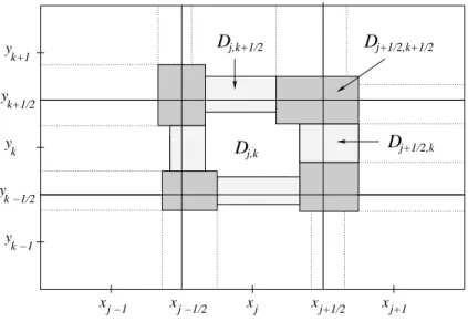
The evolution is then performed by integrating equation (4.1) over the nonuniform

control volumes Dj,k, Dj+1 2,k, Dj,k+ 1 2, and Dj+ 1 2,k+ 1

2, outlined in Figure 4.1. These domains

are determined based on the one-sided local speeds of propagation, which can be estimated, for example, by a+ j+1 2,k := maxnλN ¡ A(uW j+1,k) ¢ , λN ¡ A(uE j,k) ¢ , 0o, b+ j,k+1₂ := max n λN ¡ B(uS j,k+1) ¢ , λN ¡ B(uN j,k) ¢ , 0 o , a−_j+1 2,k := min n λ1 ¡ A(uW_j+1,k)¢, λ1 ¡ A(uE_j,k)¢, 0 o , b− j,k+1₂ := min n λ1 ¡ B(uS j,k+1) ¢ , λ1 ¡ B(uN j,k) ¢ , 0 o . (4.4)

Here, λ1 < λ2 < . . . < λN are the N eigenvalues of the corresponding Jacobians, A := ∂f_∂u

and B := _∂u∂g, and the point values of the piecewise linear reconstruction (4.2) are given by

uE(W)_j,k := ¯un j,k ± ∆x 2 (ux) n j,k, u N(S) j,k := ¯unj,k± ∆y 2 (uy) n j,k.

We refer the reader to [12, 16] for the details.

After the evolution step, the solution at time t = tn+1_{will be realized by the intermediate}

cell averages, { ¯wn+1 j,k }, { ¯wj+n+11 2,k }, { ¯wn+1 j,k+1 2 }, and { ¯wn+1 j+1 2,k+12

}, over the corresponding domains D. To complete the step of a fully-discrete scheme, one will then need to project these data back onto the original grid. This will require another piecewise linear reconstruction,

e wn+1_{(x, y) :=}X j,k h e wn+1 j,k (x, y)

χ

χ

χ

χ

2,k+12(x, y)} are the linear pieces, and

x_{j −1} x_{j −1/2} x_j+1/2 x_j+1 k+1/2 y y y k+1 y k Dj,k Dj+1/2,k D_j+1/2,k+1/2 D_j,k+1/2 x_j y k −1 k −1/2

Figure 4.1: Nonuniform control volumes in the 2-D set-up.

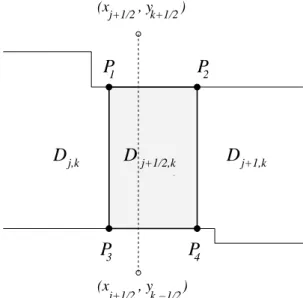
The linear pieces over the side domains, D_j+1

2,k and Dj,k+12, should be carefully chosen in

order to reduce numerical dissipation (compared with the schemes in [12, 16]). For instance,

let us consider D_j+1

2,k, see Figure 4.2. Since the length of its x-side is proportional to ∆t,

namely, |P2− P1| = |P4− P3| = (a+_j+1

2,k− a − j+1

2,k)∆t, the x-slope of the correspoding linear

piece, (wx)n+1_j+1

2,k, should be proportional to ∆w/∆t rather than to ∆w/∆x. This can be

achieved by a complete analogy with the 1-D case. We first use the Taylor expansions to

predict the values of the solution at the corners of D_j+1

2,k:

un+1(Pi) = eu(Pi, tn) − ∆t

h

f (eu(Pi, tn))_x+ g(eu(Pi, tn))_y

i

, i = 1, 2, 3, 4. (4.5)

If any of these values, say un+1_(P

i0) is not between the cell averages ¯wn+1j,k and ¯wn+1j+1,k, we

would prevent oscillation by setting

un+1_(P i0) :=    ¯ wn+1 j,k , if i0 = 1 or 3, ¯ wn+1_j+1,k, if i0 = 2 or 4.

Using the evolved values at the corners, we construct a piecewise linear interpolant over

the domain D_j+1 2,k, ¯ wn+1 j+1₂,k+ (ux) n+1 j+1 2,k(x − x n+1 j+1₂,k) + (uy) n+1 j+1 2,k(y − y n+1 j+1₂,k), (4.6) where xn+1_j+1 2,k := xj+ 1 2 + a−_j+1 2,k+ a + j+1 2,k 2 ∆t

P P P P 1 2 3 4 , y ) , y ) D_j+1,k D_j,k D_j+1/2,k (x j+1/2 k −1/2 (x_{j+1/2 k+1/2}

Figure 4.2: The side domain D_j+1

2,k. and yn+1 j+1₂,k := yk+ min(b− j,k+1₂, b − j+1,k+1₂) + max(b −_{+ j, k −} 1 2, b + j+1,k−1₂) 2 ∆t

are the coordinates of the center of D_j+1

2,k, and (ux) n+1 j+1 2,k and (uy) n+1 j+1

2,k are the x- and

y-slopes that are to be computed with the help of nonlinear limiters.

In fact, only the x-slope, (ux)n+1_j+1

2,k, should be carefully selected since in the y-direction

the size of D_j+1

2,k is proportional to ∆y and therefore, after passing to the semi-diescrete

limit, {∆t (uy)n+1_j+1

2,k} → 0 as ∆t → 0. A sharp nonoscillatory reconstruction is obtained by

taking (ux)n+1_j+1 2,k = minmod à un+1_(P 2) − ¯w_j+n+11 2,k δ , ¯ wn+1 j+1 2,k − un+1_(P 1) δ , un+1_(P 4) − ¯w_j+n+11 2,k δ , ¯ wn+1 j+1 2,k − un+1_(P 3) δ ! , δ = |P2− P1| 2 = ∆t 2 (a + j+1₂,k − a − j+1₂,k).

This slope selection helps to prevent oscillations at the corners of D_j+1

2,k, which is enough

to make the piecewise linear reconstruction non-oscillatory.

A piecewise linear reconstruction over D_j,k+1

2 is obtained similarly, a piecewise linear

reconstruction over Dj,k will always be averaged out, and no particulars of the piecewise

linear reconstruction over the corner domains, D_j+1

2,k+ 1

2, will affect the resulting

As we have mentioned in the beginning of this section, we are only interested in the 2-D semi-discrete scheme. So, we now pass to the semi-discrete limit (∆t → 0) along the lines of [12]. The resulting 2-D semi-discrete central-upwind scheme will then be obtained in the following flux form:

d dtu¯j,k(t) = − Hx j+1 2,k (t) − Hx j−1 2,k (t) ∆x − H_j,k+y 1 2 (t) − H_j,k−y 1 2 (t) ∆y , (4.7)

where the second-order numerical fluxes are

Hx j+1₂,k(t) := a+ j+1 2,k f (uE j,k) − a−_j+1 2,k f (uW j+1,k) a+ j+1₂,k− a − j+1₂,k + a+ j+1 2,k a− j+1 2,k " uW j+1,k− uEj,k a+ j+1₂,k− a − j+1₂,k − qx j+1₂,k # , (4.8) and H_j,k+y 1 2 (t) := b + j,k+1 2 g(uN j,k) − b−j,k+1 2 g(uS j,k+1) b+_j,k+1 2 − b − j,k+1 2 + b+ j,k+1 2 b− j,k+1 2 " uS j,k+1− uNj,k b+_j,k+1 2 − b − j,k+1 2 − qy_j,k+1 2 # . (4.9)

Similarly to the 1-D case, we would call qx

j+1

2,kand q

y j,k+1

2

the dissipation “correction” terms. They are given by

qx_j+1 2,k = 1 2∆t→0lim n ∆t(ux)n+1_j+1 2,k o = (4.10) = minmod à uNW j+1,k− wintj+1 2,k a+_j+1 2,k− a − j+1 2,k , w int j+1 2,k− u NE j,k a+_j+1 2,k − a − j+1 2,k ,u SW j+1,k− wintj+1 2,k a+_j+1 2,k− a − j+1 2,k , w int j+1 2,k− u SE j,k a+_j+1 2,k− a − j+1 2,k ! , q_j,k+y 1 2 = 1 2∆t→0lim n ∆t(uy)n+1_j,k+1 2 o = (4.11) = minmod à uSW j,k+1− wj,k+int 1 2 b+ j,k+1₂ − b − j,k+1₂ , w int j,k+1 2 − u NW j,k b+ j,k+1₂ − b − j,k+1₂ ,u SE j,k+1− wintj,k+1 2 b+ j,k+1₂ − b − j,k+1₂ , w int j,k+1 2 − u NE j,k b+ j,k+1₂ − a − j,k+1₂ ! , where wint j+1₂,k = _∆t→0lim w¯ n+1 j+1₂,k = a+ j+1₂,ku W j+1,k− a−_j+1 2,k uE j,k− n f (uW j+1,k) − f (uEj,k) o a+ j+1₂,k− a − j+1₂,k , wint_j,k+1 2 = ∆t→0lim w¯ n+1 j,k+1 2 = b+_j,k+1 2u S j,k+1− b−_j,k+1 2u N j,k− n g(uS j,k+1) − g(uNj,k) o b+ j,k+1 2 − b− j,k+1 2 , (4.12) and uNE

j,k, uNWj,k , uSEj,k, and uSWj,k are the corresponding corner point values of the piecewise

linear reconstruction (4.2) in the (j, k)th cell: uNE(NW)_j,k := ¯un_j,k± ∆x 2 (ux) n j,k+ ∆y 2 (uy) n j,k, u SE(SW) j,k := ¯unj,k± ∆x 2 (ux) n j,k− ∆y 2 (uy) n j,k.

Remarks.

1. Note that we are interested in the second-order scheme, and thus Simpson’s rule, used in the evaluation of the spatial integrals in [12], can be replaced with the second-order midpoint rule (see also [16]). However, our 2-D scheme (4.7)–(4.12) is still genuinely multidimensional since the computation of the “correction” terms cannot be carried out in the “dimension-by-dimension” manner.

2. As in the 1-D case, the only difference between the new 2-D central-upwind scheme

and the 2-D second-order scheme from [12] is in the “correction” terms qx

j+1 2,k and

qy_j,k+1

2

in (4.8) and (4.9), respectively. These terms help to reduce dissipation without risking big oscillations. Yet, when multidimensional systems are solved, one cannot completely avoid oscillations, and if their size gets larger than it would be acceptable,

one may increase the dissipation a little bit by multiplying qx

j+1 2,k and q_j,k+y 1 2 by a constant α < 1.

3. The system of ODEs (4.7) should be solved by a stable ODE solver. In our numerical experiments, we have used the third-ordr SSP Runge-Kutta method.

5

Numerical Experiments

In §5.1 and §5.2 below, we present numerical solutions for the gas dynamics equations for ideal gases, ∂ ∂t     ρ ρu ρv E     +_∂x∂     ρu ρu2_{+ p} ρuv u(E + p)     +_∂y∂     ρv ρuv ρv2_{+ p} v(E + p)     = 0, p = (γ − 1) h E −ρ 2(u 2_{+ v}2₎i_. (5.1) Here ρ, u, v, p and E are the density, the x- and y-velocities, the pressure and the total energy, respectively.

5.1

One-Dimensional Euler Equations of Gas Dynamics

In this subsection, we test our new semi-discrete central-upwind scheme with 1-D Euler system, where

u = (ρ, ρu, E)T_,

f (u) = (ρu, P + ρu2_{, u(E + P ))}T_{, (5.2)}

augmented with the state equation P = (γ − 1)(E − 1

2ρu2). Here ρ, u, P and E are

Several test problems have been checked. We report here three examples with significant difference.

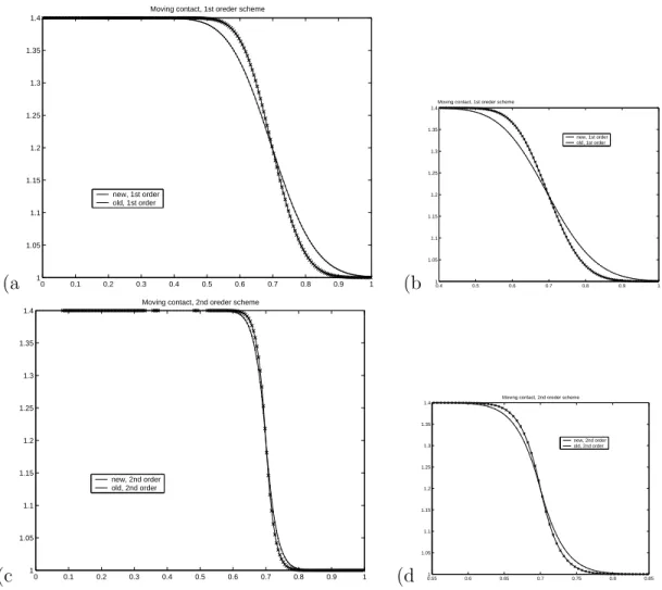
Example 1: Moving Contact Wave

In this example, we apply the schemes to the 1D Euler system (5.2) with Riemann initial data

(ρ, u, p)(x, 0) = ½

(1.4, 0.1, 1), x < 0.5,

(1, 0.1, 1), x > 0.5,

which is an example of a single contact discontinuity. We compute the approximate solution up to time T = 2, using 200 grid points on the domain [0, 1]. In Figure 5.1, we show the density plots obtained by both NEW and OLD schemes at time T = 2. Near the location of discontinuity, the graph by our new scheme clearly illustrates sharper result.

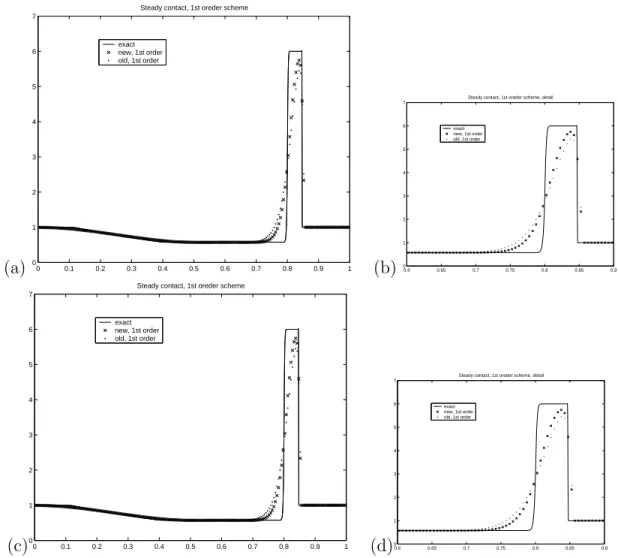
Example 2: A Stationary Contact Wave and a Travelling Shock and Rarefaction In this example, we solve 1D Euler system (5.2) with another Riemann initial data

(ρ, u, p)(x, 0) = ½

(1, −19.59745, 1000), x < 0.8,

(1, −19.59745, 0.01), x > 0.8,

which consists of a stationary contact wave, a travelling shock and a travelling rarefaction wave. We use 200 grid points and compute the solution at a final time T = 0.012 on the domain [0, 1]. The graph of density is presented in Figure 5.2, and it shows, again, sharper result obtained by our new scheme near the location of contact wave. Note that there is no significant difference near the rarefaction wave.

(a 10 0.1 0.2 0.3 0.4 0.5 0.6 0.7 0.8 0.9 1 1.05 1.1 1.15 1.2 1.25 1.3 1.35 1.4

Moving contact, 1st oreder scheme

new, 1st order old, 1st order (b 10.4 0.5 0.6 0.7 0.8 0.9 1 1.05 1.1 1.15 1.2 1.25 1.3 1.35 1.4

Moving contact, 1st oreder scheme

new, 1st order old, 1st order (c 10 0.1 0.2 0.3 0.4 0.5 0.6 0.7 0.8 0.9 1 1.05 1.1 1.15 1.2 1.25 1.3 1.35 1.4

Moving contact, 2nd oreder scheme

new, 2nd order old, 2nd order (d 0.551 0.6 0.65 0.7 0.75 0.8 0.85 1.05 1.1 1.15 1.2 1.25 1.3 1.35 1.4

Moving contact, 2nd oreder scheme

new, 2nd order old, 2nd order

Figure 5.1: Example 1: Moving Contact Wave. (a,b) by 1st order schemes; (c,d) by 2nd order schemes. (b) and (d) are zoom-in figures of (a) and (c) respectively. Final time = 2 with 200 grid points

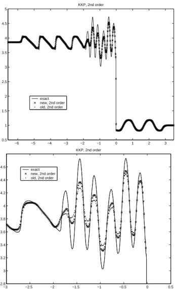
Example 3:

In this example, we compute the solution of 1D Euler system (5.2) with the initial data

(ρ, u, p)(x, 0) =    (3.857143, −0.920279, 10.33333), x < 0, (1 + ε sin(5x), −3.549648, 1.00000), 0 < x < 10, (1.000000, −3.549648, 1.00000), x ≥ 10,

corresponding to a density perturbation running leftwards into a stationary shock of Mach

number Ms = 3. This calculation has the numerical ‘flavor’ of an acoustic wave, propagating

through a steady discontinuous flow field. We take ε = 0.2 and present the solution at time T = 2.

(a) 00 0.1 0.2 0.3 0.4 0.5 0.6 0.7 0.8 0.9 1 1 2 3 4 5 6 7

Steady contact, 1st oreder scheme

exact new, 1st order old, 1st order (b) 00.6 0.65 0.7 0.75 0.8 0.85 0.9 1 2 3 4 5 6 7

Steady contact, 1st oreder scheme, detail

exact new, 1st order old, 1st order (c)00 0.1 0.2 0.3 0.4 0.5 0.6 0.7 0.8 0.9 1 1 2 3 4 5 6 7

Steady contact, 1st oreder scheme

exact new, 1st order old, 1st order (d)00.6 0.65 0.7 0.75 0.8 0.85 0.9 1 2 3 4 5 6 7

Steady contact, 1st oreder scheme, detail

exact new, 1st order old, 1st order

Figure 5.2: Example 2: Steady Contact Wave. (a,b) by 1st order schemes; (c,d) by 2nd order schemes. Final time = 0.012 with 200 grid points

Both solutions are obtained on a 1600 point mesh on domain [−9, 11], and compared with a fine grid reference solution using 20000 points.

−6 −5 −4 −3 −2 −1 0 1 2 3 0.5 1 1.5 2 2.5 3 3.5 4 4.5 5 KKP, 2nd order exact new, 2nd order old, 2nd order −3 −2.5 −2 −1.5 −1 −0.5 0 0.5 2.8 3 3.2 3.4 3.6 3.8 4 4.2 4.4 4.6 KKP, 2nd order exact new, 2nd order old, 2nd order

Figure 5.3: Example 3: at final time 2, ε = 0.2 with grid points 1600

5.2

2-D Euler Equations of Gas Dynamics

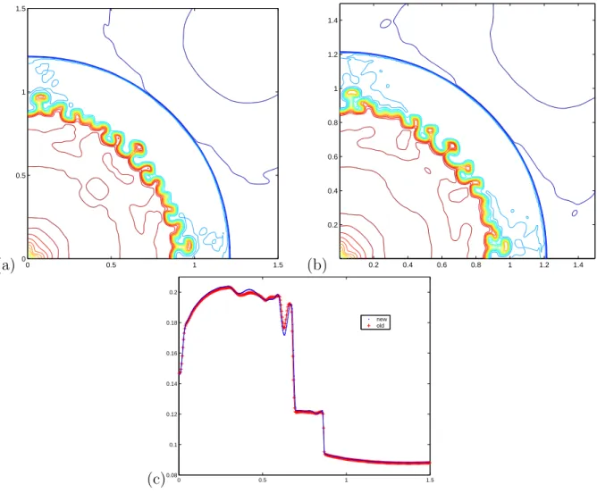
Example 2: Explosion

In this example, we compute the so-called explosion problem proposed in [27, 22], which is a radial symmetric 2D problem with higher density and higher pressure inside the initial circular region. Indeed, the physical domain [−1.5, 1.5] × [−1.5, 1.5] is separated by a circle of radius r = 0.4 centered at the origin (0, 0). Inside the circle, density and pressure are

ρin = 1, pin = 1 and ρout = 0.1, pout = 0.1 outside. The gas is initially at rest. In practice,

(a) 00 0.5 1 1.5 0.5 1 1.5 (b) 0.2 0.4 0.6 0.8 1 1.2 1.4 0.2 0.4 0.6 0.8 1 1.2 1.4 (c)0.080 0.5 1 1.5 0.1 0.12 0.14 0.16 0.18 0.2 new old

Figure 5.4: Example 5: explosion. Contours (a)and (b) are by new and old schemes respectively. (c) comparison of new and old scheme along the 45 degree radial line. Mesh size is 400×400. Final time is 3.2

Acknowledgment: The work of A. Kurganov was supported in part by the NSF Grant DMS-0310585. The work of C.T. Lin was supported in part by the NSC grants NSC 90-2115-M-126-003 & 91-2115-M-126-001. Part of the work was done when the authors visited the National Center for Theoretical Sciences at the National Tsing Hua University, Hsinchu, Taiwan and when CT visited Tulane University. We would like to thank the Center for the provided support.

References

Nessyahu-Tadmor pour une ´equation hyperbolique `a deux dimensions d’espace, C.R. Acad. Sci. Paris, t. 320, s´erie I (1995), pp. 85–88.

[2] P. Arminjon, M.-C. Viallon and A. Madrane, A finite volume extension of the Lax-Friedrichs and Nessyahu-Tadmor schemes for conservation laws on unstructured grids, Int. J. Comput. Fluid Dyn., 9 (1997), pp. 1–22.

[3] S. Bryson, A. Kurganov, D. Levy and G. Petrova, Compressed semi-discrete central-upwind schemes for Hamilton-Jacobi equations, submitted to SIAM J. Nu-mer. Anal.

[4] K.O. Friedrichs and P.D. Lax, Systems of conservation equations with a convex extension, Proc. Nat. Acad. Sci., 68 (1971), pp. 1686–1688.

[5] S. Gottlieb, C.-W. Shu and E. Tadmor, Strong stability-preserving high order time discretization methods, SIAM Review, 43 (2001), pp. 89–112.

[6] A. Harten and S. Osher, Uniformly high-order accurate nonoscillatory schemes, I, SIAM J. Numer. Anal., 24 (1987), pp. 279–309.

[7] G.-S. Jiang, D. Levy, C.-T. Lin, S. Osher and E. Tadmor, High-resolution nonoscillatory central schemes with nonstaggered grids for hyperbolic conservation laws, SIAM J. Numer. Anal., 35 (1998), pp. 2147–2168.

[8] G.-S. Jiang and E. Tadmor, Non-oscillatory central schemes for multidimen-sional hyperbolic conservation laws, SIAM J. Sci. Comput., 19 (1998), pp. 1892–1917. [9] S. Karni, E. Kirr, A. Kurganov and G. Petrova, Compressible two-phase flows by central and upwind schemes, submitted to M2AN Math. Model. Numer. Anal.

[10] A. Kurganov and D. Levy, Third-order semi-discrete central scheme for con-servation laws and convection-diffusion equations, SIAM J. Sci. Comput., 22 (2000), pp. 1461–1488.

[11] A. Kurganov and D. Levy, Central-upwind schemes for the Saint-Venant system, M2AN Math. Model. Numer. Anal., 36 (2002), pp. 397–425.

[12] A. Kurganov, S. Noelle and G. Petrova, Semi-discrete central-upwind scheme for hyperbolic conservation laws and Hamilton-Jacobi equations, SIAM J. Sci. Comput., 23 (2001), pp. 707–740.

[13] A. Kurganov and G. Petrova, A third-order semi-discrete genuinely multi-dimensional central scheme for hyperbolic conservation laws and related problems, Numer. Math., 88 (2001), pp. 683–729.

[14] A. Kurganov and G. Petrova, Central schemes and contact discontinuities, M2AN Math. Model. Numer. Anal., 34 (2000), pp. 1259–1275.

[15] A. Kurganov and E. Tadmor, New high-resolution central schemes for nonlin-ear conservation laws and convection-diffusion equations, J. of Comput. Phys., 160 (2000), pp. 241–282.

[16] A. Kurganov and E. Tadmor, Solution of two-dimensional Riemann problems for gas dynamics without Riemann problem solvers, Numer. Methods Partial Differ-ential Equations, to appear.

[17] B. van Leer, Towards the ultimate conservative difference scheme, V. A second order sequel to Godunov’s method, J. of Comput. Phys., 32 (1979), pp. 101–136. [18] D. Levy, G. Puppo and G. Russo, Central WENO schemes for hyperbolic

sys-tems of conservation laws, M2AN Math. Model. Numer. Anal., 33 (1999), pp. 547– 571.

[19] D. Levy, G. Puppo and G. Russo, Compact central WENO schemes for multi-dimensional conservation laws, SIAM J. Sci. Comput., 22 (2000), pp. 656–672. [20] K.-A. Lie and S.Noelle, On the artificial compression method for second-order

nonoscillatory central difference schemes for systems of conservation laws, SIAM J. Sci. Comput., 24 (2003), pp. 1157–1174.

[21] X.-D. Liu and E. Tadmor, Third order nonoscillatory central scheme for hyper-bolic conservation laws, Numerische Mathematik, 79 (1998), pp. 397–425.

[22] R. Liska and B. Wendroff, Comparison of Several Difference Schemes on 1D and 2D Test Problems for the Euler Equations, SIAM J. Sci. Comput., 25 (2004), pp. 995–1017.

[23] H. Nessyahu and E. Tadmor, Non-oscillatory central differencing for hyperbolic conservation laws, J. Comput. Phys., 87 (1990), pp. 408–463.

[24] C. W. Schulz-Rinne, Classification of the Riemann problem for two-dimensional gas dynamics, SIAM J. Math. Anal., 24 (1993), pp. 76–88.

[25] C. W. Schulz-Rinne, J. P. Collins and H. M. Glaz, Numerical solution of the Riemann problem for two-dimensional gas dynamics, SIAM J. Sci. Comput., 14 (1993), pp. 1394–1414.

[26] P.K. Sweby, High resolution schemes using flux limiters for hyperbolic conservation laws, SIAM J. Numer. Anal., 21 (1984), pp. 995–1011.

[27] E.F. Toro, Riemann Solvers and Numerical Methods for Fluid Dynamics: A Prac-tical Introduction, 2nd edition, Springer,(1999).