What Are the Important Factors for NBA Player Salaries in 2017?

What Are the Important Factors for NBA Player Salaries in 2017?

Author(s): 鄭哲睿(Zhe-Rui Zheng)、朱天婕(Tian-Jie Zhu)、林翰博(Han-Bo Lin)、薛藝湛(Yi-Zhan Xue)、周佳玉(Jia-Yu Zhou)

Class: 2nd year of SJSU-FCU 2+2 Bachelor's Program in Business Analytics Student ID: D0571987、D0571926、D0571960、D0571930、D0572026 Course: Introduction to Data Analytics

Instructor: Dr. Cathy W. S. Chen

Department: International School of Technolog y and Management Academic Year: Semester 1, 2017-2018

Abstract

It is of great interest to identify the factors that influence the salaries of National

Basketball Association (NBA) players. This study examines the 2017-2018 wages of

100 NBA players which are randomly selected by the SAS software based on their

career performance variables using a multiple linear regression. There are 28

explanatory variables which include age, 3-point field goals per game and free throws

per game. The multiple regression analysis is conducted to determine the explanatory

variables which are helpful in predicting the salaries of NBA players. Five methods

for model selection are used, these include forward selection, backward elimination,

stepwise selection, adjusted R-square selection method and C(p) method. All five

methods demonstrated similar results. Results indicated that variables such as games

started, field goals per game, total rebounds per game, personal fouls per game, also

the terms of contract used, have a significant correlation with salary.

Keyword：

Table of Content

I. Introduction... 5

II. Method... 6

i. Data Description ... 6

ii. Scatter Plot and Basic Statistics ... 7

iii. Variable Explanation ... 9

iv. Variable Selection ... 11

v. Model Representation ... 14

III. Model Analysis ... 16

i. Outliers Analysis ... 16

ii. Influential Point Analysis ... 16

iii. Four Assumption Verification ... 18

III. Findings and Discussion ... 21

IV. Appendix ... 22

i. Data Resources ... 22

ii. References ... 22

iii. Outlier and Influential Point Analysis ... 22

List of Figures

Figure 1: Scatter Plot Between Salary and Age ... 25

Figure 2: Scatter Plot Between Salary and G ... 25

Figure 3: Scatter Plot Between Salary and GS ... 25

Figure 4: Scatter Plot Between Salary and MP ... 25

Figure 5: Scatter Plot Between Salary and FG ... 25

Figure 6: Scatter Plot Between Salary and FGA... 25

Figure 7: Scatter Plot Between Salary and THP ... 26

Figure 8: Scatter Plot Between Salary and THPA... 26

Figure 9: Scatter Plot Between Salary and THPPer ... 26

Figure 10: Scatter Plot Between Salary and TWP ... 26

Figure 11: Scatter Plot Between Salary and TWPA ... 26

Figure 12: Scatter Plot Between Salary and TWPPer ... 26

Figure 13: Scatter Plot Between Salary and eFGPer ... 27

Figure 14: Scatter Plot Between Salary and FTA ... 27

Figure 15: Scatter Plot Between Salary and FTPer ... 27

Figure 16: Scatter Plot Between Salary and ORB ... 27

Figure 17: Scatter Plot Between Salary and DRB ... 27

Figure 18: Scatter Plot Between Salary and FGPer ... 27

Figure 19: Scatter Plot Between Salary and TRB ... 28

Figure 20: Scatter Plot Between Salary and FT ... 28

Figure 21: Scatter Plot Between Salary and STL ... 28

Figure 22: Scatter Plot Between Salary and AST ... 28

Figure 23: Scatter Plot Between Salary and BLK ... 28

Figure 24: Scatter Plot Between Salary and TOV ... 28

Figure 25: Scatter Plot Between Salary and PFA... 29

List of Tables

Table 1: Descriptive statistics for the 100 NBA players in the 2016-2017 season ... 8

Table 2: Variance inflation factor for the variables ... 14

Table 3: Influential points for the variables ... 17

Table 4: Test for Location Mu0=0 ... 19

Table 5: Heteroscedasticity Test ... 19

Table 6: Durbin-Watson Test ... 20

Chapter 1

Introduction

With more companies sponsoring the NBA and a higher salary cap, an increasing

number of players are asking for a higher salary. Furthermore, there is already a huge

salary gap between NBA players. In the 2017-2018 season, the lowest salary drawn is

25,000 dollars. However, Stephen Curry earned the highest salary in the NBA at

34,682,550 dollars, which is almost one thousand four hundred times that of the

lowest.

Moreover, aside from the huge salary gap, overpaid players exist in every team.

Forbes magazine listed Carmelo Anthony as the most overpaid player of 2018. As his

pace to produce wins stands at negative 1.3, this means that the team is more likely to

lose the game if he is playing. In addition to that, his field goal percentage, rebounds

and assists are all below career average. With such lousy performances, his salary

remains very high by NBA standards at 26,243,760 dollars, making it the twelfth

highest in the NBA. This financial arrangement undoubtedly influences the balance of

the team. With an overpaid player on the books, the team manager would find it

difficult to trade for better players with the limit on the salary cap. As a fan of the

NBA, I am constantly curious whether it is worthwhile to pay such a high salary and whether the players’ performance out on the basketball court influences their salary?

Kaggle to find a regression line in the data to predict the players’ salaries.

Furthermore, I will also focus on unexpected factors which may influence players’

salaries.

Regarding the methodology, due to the large number of variables in the data set, We

first selected several variables that might be useful. Then by using a scatter plot, we

would have a brief idea of the relationship between the response variable and the

explanatory variables. Later on, We use the five methods entirely which includes

stepwise selection, forward selection, backward elimination, adjusted R-square

selection method and C(p) selection method to choose the variables for the final

model. Lastly, we made sure that no multicollinearity exists in the final model and

verified all four assumptions.

Chapter 2

Method

2.1 Data Description

The data set we selected was based on the 2016-2017 season. The website named

Basketball Reference provided the entire data set. For players included in the data set,

this study will only analyse those whose number of games played is more than 25.

Due to the amount of games played being too small, the statistics does not clearly

reflect the players’ ability, so the regression model cannot accurately predict their

used. According to the rules, the rookies’ salaries are constrained by the rookie salary

cap. Hence if their performance is better as compared to the latter season, their

salaries remain stagnant rather than indicating an increase in wages. Lastly, 100

players will be randomly selected from the entire data set.

2.2 Scatter Plot and Basic Statistics

Figures 4, 5, 6, 10, 11, 14, 17, 20, 24, 26 in the appendix present the MP (minutes

played per game), FG (field goals per game), FGA (field goal attempts per game),

TWP (2-point field goals per game), TWPA (2-point field goal attempts per game),

FTA (free throw attempts per game), DRB (defensive rebounds per game), FT (free

throws per game), TOV (turnovers per game) and PSG (points per game), all of which

have a positive correlation with salary. For other variables, the scatter plot does not

indicate a clear relationship with salary levels. Moreover, the scatter plot did not

exhibit any significant outliers and it was not necessary to delete any data points in

this step.

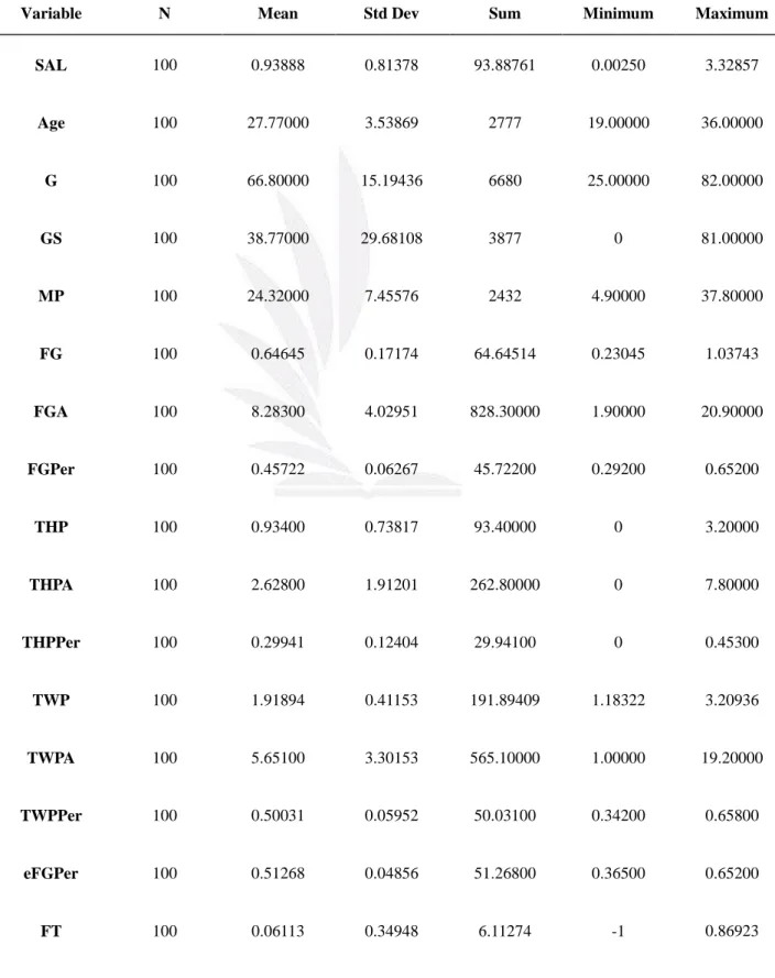
Table 1 illustrates the basic statistics which include the mean, average, standard

deviation, minimum and maximum for each variable. Several of the minima variable

are equal to zero; for example, in the case of the GS (games started) variable, it means

step, a detailed explanation will be outlined along with the processing method for each

variable.

Table 1 Descriptive statistics for the 100 NBA players in the 2016-2017 season

Variable N Mean Std Dev Sum Minimum Maximum

SAL 100 0.93888 0.81378 93.88761 0.00250 3.32857 Age 100 27.77000 3.53869 2777 19.00000 36.00000 G 100 66.80000 15.19436 6680 25.00000 82.00000 GS 100 38.77000 29.68108 3877 0 81.00000 MP 100 24.32000 7.45576 2432 4.90000 37.80000 FG 100 0.64645 0.17174 64.64514 0.23045 1.03743 FGA 100 8.28300 4.02951 828.30000 1.90000 20.90000 FGPer 100 0.45722 0.06267 45.72200 0.29200 0.65200 THP 100 0.93400 0.73817 93.40000 0 3.20000 THPA 100 2.62800 1.91201 262.80000 0 7.80000 THPPer 100 0.29941 0.12404 29.94100 0 0.45300 TWP 100 1.91894 0.41153 191.89409 1.18322 3.20936 TWPA 100 5.65100 3.30153 565.10000 1.00000 19.20000 TWPPer 100 0.50031 0.05952 50.03100 0.34200 0.65800 eFGPer 100 0.51268 0.04856 51.26800 0.36500 0.65200 FT 100 0.06113 0.34948 6.11274 -1 0.86923

FTA 100 2.06700 1.65682 206.70000 0.10000 8.70000 FTPer 100 0.74915 0.12232 74.91500 0.27300 1.00000 ORB 100 0.99400 0.86676 99.40000 0 4.30000 DRB 100 0.44702 0.26002 44.70178 -0.69897 1.01284 TRB 100 4.26800 2.58167 426.80000 0.20000 14.10000 AST 100 1.39256 0.57188 139.25616 0.44721 3.27109 STL 100 0.78600 0.39467 78.60000 0 2.00000 BLK 100 0.44300 0.38462 44.30000 0 2.10000 TOV 100 0.03666 0.24264 3.66553 -0.69897 0.61278 PFA 100 1.89200 0.61162 189.20000 0.20000 3.30000 PSG 100 10.07000 5.39999 1007 2.20000 27.30000

2.3 Variable Explanation

This section will explain one response variable and twenty-eight explanatory variables

which are of interest along with the methodology through which the variables are

processed.

Response Variable

SAL is considered the response variable. SAL is represents the NBA players’

annual salary in the denomination of ten million.

1. Age: Age of Player at the start of the season, February 1st

2. G: Games

3. GS: Games Started

4. MP: Minutes Played Per Game

5. FG: Field Goals Per Game

6. FGA: Field Goal Attempts Per Game

7. FGPer: Field Goal Percentage

8. THP: 3-Point Field Goals Per Game

9. THPA: 3-Point Field Goal Attempts Per Game

10. THPPer: FG% on 3-pt FGAs

11. TWP: 2-Point Field Goals Per Game

12. TWPA: 2-Point Field Goal Attempts Per Game

13. TWPPer: FG% on 2-pt FGAs

14. eFGPer: Effective Field Goal Percentage, this statistic adjusts for the fact

that a 3-point field goal is worth one point more than a 2-point field goal.

15. FT: Free Throws Per Game

16. FTA: Free Throw Attempts Per Game

17. FTPer: Free Throw Percentage

19. DRB: Defensive Rebounds Per Game

20. TRB: Total Rebounds Per Game

21. AST: Assists Per Game

22. STL: Steals Per Game

23. BLK: Blocks Per Game

24. TOV: Turnovers Per Game

25. PFA: Personal Fouls Per Game

26. PSG: Points Per Game

27. Pos : Position, this is a dummy variable where six positions are included,

they are PG, SG, SF, PF, C, PF-C.

28. Signed Using: this is a dummy variable where six signs are included, they

are FRP (first round pick), BR (Bird Right), CS (Cap Space), MS (Minimum

Salary), Others (Signed like MLE, Bi-annual Exception are included) and None.

However as aforementioned, players with the FRP sign will not be used.

2.4 Variable Selection

Five methods were utilised in the selection of variables; stepwise selection, backward

elimination, forward selection, adjusted R-square selection method and C(p) selection

method. However, for the adjusted R-square selection method and C(p) selection

selection, backward elimination and forward selection to choose the variable. To

obtain a highly adjusted R-square and to avoid multicollinearity at the same time, it

was decided that the variables would be selected through stepwise selection.

Backward Elimination

Backward Elimination begins with a regression on all variables. Following that,

every independent variable will be examined, thereby removing the variables

with the smallest p-value. This process is repeated until no variables can be

removed.

Thirteen variables are chosen through this method. They are Signed Using, GS,

MP, FGPer, THPPer, TWPA, eFGPer, FTA, FT, STL, BLK, PFA, PSG. The

is set at 0.15

Forward Selection

Forward Selection begins with no variables. This method examines every

variable and those with the most significant contribution will be added to the

model. Following that, a new regression is run with a lesser variable. The step

will be repeated until no variables can be selected.

Six variables are chosen through this method. They are Signed Using, GS, THP,

FTA, TRB, PFA. The is set at 0.15

In Stepwise Selection, a variable can be added or deleted from the model several

times before the final model is attained, and is also dependent on the other

variables in the model.

Six variables are chosen through this method. They are Signed Using, GS, THP,

FTA, TRB, PFA. The is set at 0.15 for both sides.

Adjusted R-square Selection Method

Adjusted R-square Selection Method lists all possible models and calculates the

adjusted R-square for each model. The model with the largest adjusted R-square

will be considered the best model.

PG, SG, CS, MS, GS, MP, FGA, FGPer, THP, THPPer, eFGPer, FTA, FT, STL,

BLK, PFA, PSG are the variables chosen through this method. However, in the

adjusted R-Square Selection Method, grouping information is not considered.

Thus, the models selected by this method will not be used.

C(p) Selection Method

Similar to the Adjusted R-square Selection model, the C(p) Selection Method

also lists all possible models as the C(p) value is calculated for each model. The

model with the smallest C(p) value will be considered the best model.

CS, MS, GS, FGA, eFGPer, TRB, PFA, PSG are the variables chosen by this

selected by this method will not be used.

2.5 Model Representation

The final model was selected through stepwise selection. The final model is shown

below.

= 0.1302 + 0.0074 GS + 0.109 THP + 0.2581 FTA + 0.6653 TRB - 0.2319 PFA + 0.0572 BR + 0.1909 CS - 0.3384 MS.

As the regression model shows, players’ salary increased along with an increase in the

variables such as GS, THP, FTA, and TRB. However, a higher number of personal

fouls in a game actually corresponds with a decrease in salary. Furthermore, players

with the sign Cap Space are more likely to earn a higher salary.

VIF

Multicollinearity exists if there is a substantial correlation between independent

variables. To diagnose multicollinearity in this model, the variance inflation

factor is used. If the factor is larger than 10, it can be assumed that

multicollinearity exists in the model. As shown in table 2, there is no

multicollinearity in the final model.

Table 2 Variance inflation factor for the variables

Parameter Estimates

Variable

Parameter Estimate

Standard Error t Value Pr > |t|

Variance Inflation

Intercept _{0.13020 0.16386 0.79 0.4290} 0 GS 0.00735 0.00194 3.80 0.0003 2.03018 THP 0.10898 0.06611 1.65 0.1028 1.46239 FTA 0.25810 0.03178 8.12 <.0001 _1.70243 TRB 0.06526 0.02450 2.66 0.0092 2.45638 PFA -0.23193 0.08840 -2.62 0.0102 1.79504 BR 0.05715 0.15625 0.37 0.7154 2.51203 CS 0.19087 0.13227 1.44 0.1525 2.67373 MS -0.33838 0.16005 -2.11 0.0373 1.67774 Others -0.08458 0.18564 -0.46 0.6498 1.57305 Adjusted R-square

The adjusted R-square is a modified version of R-square for the number of

predictors in the model. The adjusted R-square can be calculated with the

following formula:

The adjusted R-square for the final model is 0.7565. In other words, 75.65% of

Chapter 3

Model Analysis

This section mainly carries out the outliers analysis, the influential point analysis and

the verification of four assumptions.

3.1 Outliers Analysis

An observation that is markedly different from, or atypical of, the rest of the

observations in a data set is known as an outlier. In the outlier analysis, the RStudent

and student residual variables are primarily used in the study. If the RStudent and

student residual are in excess of three, it confirms that the point is an outlier. The ninth

data point is the only outlier in the data set.

3.2 Influential Point Analysis

An observation that causes the regression estimates to be substantially different from

what they would be if the observation was removed from the data set is called an

influential observation. Besides that, influential observations are typically outliers that

have high leverage. To judge the influential point, four entire methods are used; they are Cook’s Distance, COVRATIO, DFFITS and DFBETAS respectively. The table is

shown in the appendix. Cook’s Distance

If the Cook’s Distance is larger than 0.5, the data might be influential. However,

conclude that the , , 52nd_{, , , , are influential points.}

DFFITS

If , it can be concluded that the data is influential. Within

the data set, if DFFITS is larger than 0.63or smaller than -0.63, the data can be

considered as an influential point. In this data set, we can conclude that the ,

, , , , are influential points.

COVRATIO

If or , then the point is

considered influential. In the data set, if the COVRATIO value is not between

1.3 and 0.7, the data point can be defined as an influential point. Finally, it can

be concluded that , , 51st, , , are influential points

DFBETAS

For these data sets, an observation is deemed influential if .

In the data set, if the absolute value of DFBETAS is larger than 0.164, the data

point can be concluded as an influential point.

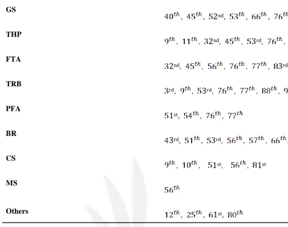
Table 3 Influential points for the variables

Variable Influential Point

GS , , 2nd_{, , ,} THP , , 2nd_{, , 3}rd_{, , 3}rd_{, ,} FTA 2nd_{, , , , , 3}rd_{, ,} TRB rd_{, , 3}rd_{, , , ,} PFA 1st_{, , ,} BR 3rd_{, , 3}rd_{, , , ,} CS , , 1st_{, , 1}st MS Others _{, , 1}st_,

In conclusion, the 9th _{point is the most likely to become the influential point. The}

player on the ninth point is Chandler Parsons. He is a very outstanding player,

especially in the 2014 season. He even set the record for the number of 3-pointers

scored in one half. NBA teams offered him a high salary package at that point in time.

However, in recent years and due to an injury, his performance has worsened and

deteriorated. Hence it is reasonable for this data point to become an influential point

and an outlier.

3.3 Four Assumption Verification

First Assumption:

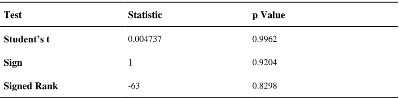
Test for Location: Mu0=0

Test Statistic p Value

Student’s t 0.004737 0.9962

Sign 1 0.9204

Signed Rank -63 0.8298

From the Student's t, Sign and Signed Rank test, all the p-values are larger than

0.05, so H0 cannot be rejected. This assumption is confirmed.

Second Assumption:

Table 5 Heteroscedasticity Test

Heteroscedasticity Test

Equation Test Statistic DF Pr > ChiSq Variable

SAL White’s Test 21.80 44 0.9980 Cross of all vars

Breusch-Pagan 9.69 9 0.3759 1, GS, THP, FTA, TRB, PFA, BR, CS, MS, Others

Shown as the table of the Heteroscedasticity test in the appendix, the p-value is

larger than 0.05. Hence we can verify this assumption. Third Assumption:

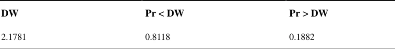
Table 6 Durbin-Watson Statistics

Durbin-Watson Statistics

DW Pr < DW Pr > DW

2.1781 0.8118 0.1882

According to Durbin-Watson Statistics, both the p-values are larger than 0.05.

Hence there is no positive or negative autocorrelation between the variables.

Fourth Assumption:

Table 7 Test for Normality

Test for Normality

Test Statistic p Value

Shapiro-Wilk 0.977189 0.0801

Kolmogorov-Smirnov 0.052831 >0.1500

Cramer-von Mises 0.041146 >0.2500

Anderson_Darling 0.335538 >0.2500

In order to verify that the residuals follow a normal distribution, four tests are

used; Shapiro-Wilk, Kolmogorov-Smirnov, Cramer-von Mises and

larger than 0.05. Hence H0 cannot be rejected and the assumption can be

verified.

In conclusion, all four assumptions can be verified. This confirms that the model can

be used to make an inference or a prediction.

Chapter 4

Findings and Discussion

This study primarily highlights the findings through a rigorous analysis of the data set

and discusses unexpected discoveries in the following step.

As the regression line is drawn, the salary is mainly related to six variables; they are

Games Started (GS), 3-Point Field Goals Per Game (THP), Free Throw Attempts Per

Game (FTA), Total Rebounds Per Game (TRB), Personal Fouls Per Game (PFA) and

Signed Use. All the variables except for Signed Use and Personal Fouls Per Game

have a positive correlation with salary, which means that a higher number for Games

Started, 3-Point Field Goals Per Game, Free Throw Attempts Per Game and Total

Rebounds Per Game, the higher the salary. Meanwhile, a higher number of Personal

Fouls Per Game will correspond with a decrease in salary. Furthermore, Signed Use is

a crucial variable in the regression model. As the model shows, players with the sign

The research also considered if the players’ performance on social media scored a

higher R-square. Every players’ Twitter account was tracked and an API provided by

Twitter allowed revealed the number of followers for each player. Following that, the

variable was added into the final model, leading to an increase in the R-square value

to 0.7621. It can be concluded that their performance on social media actually

increases the accuracy of the model whereby more data can be explained.

The variable for the number of Twitter followers also gives an idea about the players'

performance outside the basketball count and plays an essential roll in determining

salary levels. Variables such as time spent in the fitness room may also be collected in

the future to predict salary.

Chapter 5

Appendix

5.1 Data Resources

1. https://www.basketball-reference.com/leagues/NBA_2017_per_game.html (data

resource)

2. https://www.basketball-reference.com/contracts/players.html (data resource)

3. https://www.basketball-reference.com/friv/twitter.html (NBA players’ Twitter

5.2 References

1. Freund. R. J., Wilson. J. W., & Sa. P. (2006) Regression Analysis, 2nd ed 2. Knight. B. (2018) The NBA’s Most Overpaid Players 2018

3. Mason. L. J. (2004) Salaries of NBA Players: A Regression Analysis 4. Gain. C. (2017) The Most Overpaid Players and NBA Salaries