具有學習效果的流程式生產排程之最大完工時間與總完工時間最小化之研究

國 立 交 通 大 學

工業工程與管理學系

博 士 論 文

具有學習效果的流程式生產排程之最大完工時間與總

完工時間最小化之研究

Scheduling Problems to Minimize Makespan and Total

Completion Time in Flowshop Environment with

Learning Effects

研 究 生：鐘愉翔

指導教授：唐麗英 教授

洪瑞雲 教授

具有學習效果的流程式生產排程之最大完工時間與總

完工時間最小化之研究

Scheduling Problems to Minimize Makespan and Total

Completion Time in Flowshop Environment with

Learning Effects

研 究 生：鐘愉翔

Student： Yu-Hsiang Chung

指導教授：唐麗英 教授

Advisor： Dr. Lee-Ing Tong

指導教授：

洪瑞雲 教授

Advisor：

Dr. Ruey-Yun Horng

國 立 交 通 大 學

工 業 工 程 與 管 理 學 系

博 士 論 文

A Dissertation

Submitted to Department of Industrial Engineering and Management College of Management

National Chiao Tung University in partial Fulfillment of the Requirements

for the Degree of Doctor of Philosophy

in

Industrial Engineering and Management November 2011

Hsinchu, Taiwan, Republic of China

具有學習效果的流程式生產排程之最大完工時間與總完工

時間最小化之研究

研究生：鐘愉翔

指導教授：唐麗英 博士

洪瑞雲 博士

國 立 交 通 大 學

工業工程與管理學系

摘

要

在傳統的排程問題中，工作件的加工時間皆設定為固定常數，且不會因工作件在機 台上的加工順序而改變，然而當執行加工的人員因重複處理類似工作件而獲得經驗時， 工作件的加工時間會因此縮減，此現象為近年來在排程領域被廣泛討論的「學習效果 (Learning effect)」。學習效果可分類為兩種型式，分別為「依加工順序改變之學習效果

(Position-based learning effect) 」 與 「 依 已 加 工 時 間 改 變 之 學 習 效 果 (Sum-of-processing-time-based learning effect)」，在一個排程問題中，此兩種型式之學習 效果可以單獨考慮或同時考慮，由於依加工順序改變之學習效果模型為理論上的理想學 習模型，因此本論文將探討依加工順序改變之學習效果。再者，目前關於具有學習效果 的排程問題大多針對單機做探討，然而在實際製程上，許多生產環境的排程屬於多機流 程式生產排程，其問題之求解的複雜性亦高於單機生產排程問題。此外，大多數排程問 題之目的是求得最佳的工作件排序使其目標函數最小化，而最常被探討的目標函數為最 大完工時間與總完工時間。因此本論文針對依加工順序改變之學習效果探討兩個多機流 程式生產排程問題，第一個問題設定所有機台有相同的學習效果，其目標為最大完工時 間最小化；第二個問題則是依不同機台有不同的學習效果，其目標為加權整合之總完工 時間與最大完工時間最小化。 本論文對於工作件數少的問題，使用分枝界限演算法求得最佳排序，接著推導凌越 性質與下界值以增進分枝界限演算法的求解效率；對於工作件數多的問題，本論文將利

用兩個知名的啟發式演算法、模擬退火法與基因演算法來求得近似解。最後，本論文將 針對所有提出的演算法進行電腦模擬，以探討學習效果對於分枝界限演算法的求解效率 與啟發式演算法的精準性之影響。針對本論文探討之問題的電腦模擬結果，我們發現將 傳統環境中求得之最佳排序應用在具有學習效果的環境中，得到的目標函數值將比實際 的最佳目標函數值大，此現象指出學習效果對本論文提出的排程問題有顯著的影響。而 在求最佳排序時，分枝界限演算法求解的效率與學習效果的強度成正比。此外，基因演 算法為本論文提出之求近似解的演算法中最精準的。基於分枝界限演算法求解時間的分 佈變異大且呈右偏，因此本論文建議在求解時先施以分枝界限演算法，若在合理的時間 內無法求得最佳排序，則施以基因演算法求近似排序。最後，若流程式生產環境中的機 台上能指派不同的操作員，則將學習能力強的操作員指派至工作量較大的機台上能得到 較佳的目標函數值。 關鍵字：流程式生產排程、學習效果、最大完工時間、總完工時間

Scheduling Problems to Minimize Makespan and Total

Completion Time in Flowshop Environment with Learning

Effects

Students: Yu-Hsiang Chung Advisor: Dr. Lee-Ing Tong

Dr. Ruey-Yun Horng

Department of Industrial Engineering and Management,

National Chiao Tung University

ABSTRACT

In traditional scheduling problems, the processing time for a given job is assumed to be a fixed constant no matter the scheduling order of the job. However, it is noticeable that the job processing time declines as workers gain more experience. This phenomenon is called the “learning effect”. The learning effect is extensively studied in scheduling field recently, and it can be classified into two types: “the position-based learning” and “the sum-of-processing- time-based learning”. The two types of learning effect can be considered alone or simultaneously in a scheduling problem. The position-based learning is studied in this dissertation because of its model is the pure learning model in theory. In addition, most of the studies on the learning effect are focused only on single-machine setting. However, numerous real-world industrial problems belong to flowshop scheduling problems, and dealing with the flowshop scheduling problems is more complex than dealing with the single-machine problems. Most scheduling problems aim at determining an optimal sequence to minimize the objective function. The makespan and total completion time are the objective functions that are often studied. As a result, this dissertation discusses two flowshop scheduling problems with position-based learning effect. The learning effects are identical on all machines, and the purpose is to minimize the makespan in the first problem. The learning effects are distinct for different machines, and the purpose is to minimize the weighted sum of total completion time

and makespan in the second problem.

In this dissertation, the branch-and-bound algorithm is proposed to seek the optimal sequence for the small job-sized problem. Then the dominance properties and lower bounds are proposed to accelerate the procedure of the branch-and-bound algorithm. For the large job-sized problem, two well-known heuristic algorithms, simulated annealing and genetic algorithm are utilized to yield the near-optimal sequence. In the end, the simulated experiments are examined to assess the performance of the algorithms proposed in this dissertation. The computational results of the proposed problems reveal that the objective value calculated from the optimal sequence under the traditional environment is larger than the optimal objective value in the environment with learning considerations. It implies the influence of the learning effect is notable for the problems proposed in this dissertation. Furthermore, the efficiency of the branch-and-bound algorithm ascends as the learning effect enhances while seeking the optimal sequence. The proposed genetic algorithm has the best performance among all heuristic and meta-heuristic algorithms in terms of the accuracy. In addition, due to the large variance and the right skewness for the distribution of the execution time, the branch-and-bound algorithm is recommended to obtain the optimal sequence in a reasonable amount of time, or to derive the near-optimal sequence from the proposed genetic algorithm. Eventually, assigning the operator with stronger learning effect to the machine with heavier workload might derive smaller objective value while the operators are allocated in the flowshop environment.

誌

謝

經歷四年的博士研究階段，愉翔首先要感謝 唐麗英 教授與 洪瑞雲 教授兩位老師 無私的指導駑鈍的我作研究，有了兩位博學多聞的恩師寢囊相授，使本論文的內容更加 嚴謹與充實。愉翔也從兩恩師身上學到了圓融的待人處事方法，對於老師四年中的照顧 與教誨，愉翔將永遠銘記在心。 愉翔感謝論文口試委員 黎正中 教授、李榮貴 教授與 王春和 教授在本論文審查 及口試其間的辛勞，並給予寶貴的建議及鼓勵，使愉翔能在未來的研究及生涯規劃上注 入新的想法。 愉翔感謝祖父 鐘坤湖 先生、先祖母 鐘黃金女 居士、父親 鐘健倉 先生、母親 林 嫣嫣 女士及妹妹 鐘樂珊 小姐對我不變的支持與鼓勵，讓我能無後顧之憂的專心作研 究。另外也要感謝一直對愉翔抱持信心的親戚，大家的期許讓我更有努力向上的動力。 愉翔感謝碩士班的恩師 李文烱 教授與 吳進家 教授，兩位老師激發我對研究的熱 誠，讓我有機會突破自我。最後要感謝 佳煌、元銘、凱斌學長、榮弘學長與一平學長， 有了各位的陪伴與指導，使我四年的求學過程多采多姿。感謝所有幫助過我的人，愉翔 會竭盡所能的努力，不辜負大家對我的期望。

鐘愉翔

謹誌 中華民國 一百 年 十一 月于交通大學

Contents

Abstract (in Chinese) i

Abstract (in English) iii

Acknowledgements (in Chinese) v

List of Tables viii

List of Figures ix

Chapter 1 Introduction

1

1.1 Research motivation 1

1.2 Literature review 3

1.3 Research objectives and methodologies 9

Chapter 2 Algorithms

12

2.1 Branch-and-bound algorithms 12

2.2 Heuristic algorithms 15

2.3 Meta-heuristic algorithms 17

Chapter 3 Makespan minimization for m-machine flowshop scheduling

problem with position-based learning effects

22

3.1 Notations and problem statement 22

3.2 Dominance property 23

3.3 Lower bound 25

3.4 Computational results 28

Chapter 4 Bi-criteria minimization for m-machine flowshop scheduling

problem with machine- and position-based learning effects

39

4.1 Notations and problem statement 39

4.2 Dominance property 40

4.3 Lower bound 42

4.4 Computational results 44

4.5 Summary 63

Chapter 5 Concluding remarks

64

5.1. Conclusion 64

5.2 Suggestions for further studies 65

List of Tables

Table 3.1. The influence of the learning effect on optimal solution 28

Table 3.2. The performance of the property and the lower bound for the branch-and-bound algorithm 29

Table 3.3. The performance of branch-and-bound algorithm and heuristic algorithms of different parameters 31

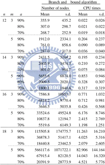
Table 3.4. The performance of branch-and-bound algorithm of different parameters after outliers elimination 34

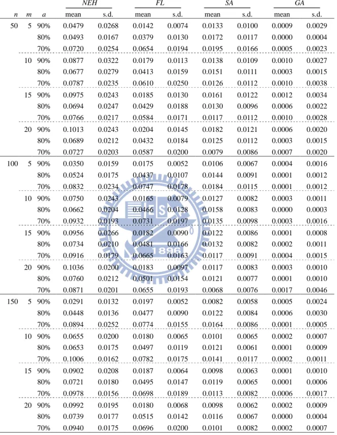
Table 3.5. The relative percentage deviation of heuristic algorithms 36

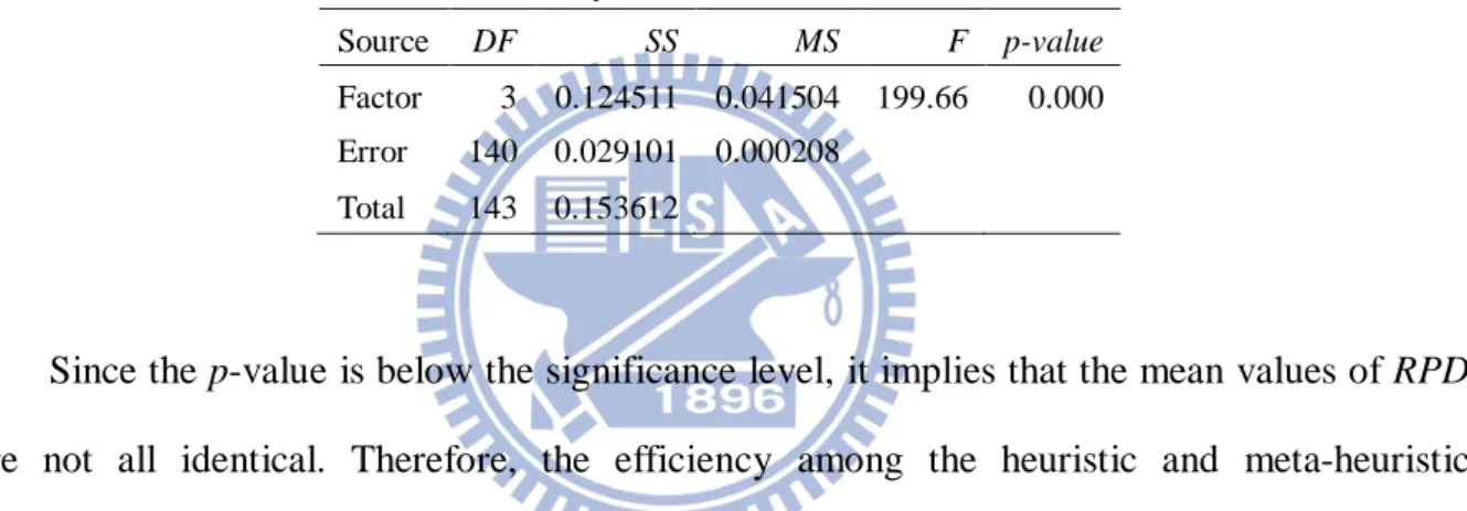
Table 3.6. One-way ANOVA for RPD of four heuristics 37

Table 3.7. Tukey-test results of four heuristics 38

Table 4.1. The index set of the learning effects 46

Table 4.2. The performance of the branch-and-bound algorithm 49

Table 4.3. The comparison among five learning patterns for the optimal objective value 52

Table 4.4. The performance of the heuristic algorithms (α =0.25) 54

Table 4.5. The performance of the heuristic algorithms (α =0.50) 55

Table 4.6. The performance of the heuristic algorithms (α =0.75) 57

Table 4.7. Two-way ANOVA of the error percentages for all heuristic algorithms 59

List of Figures

Fig 2.1. The flowchart of the proposed branch-and-bound algorithm 14

Fig 2.2. The flowchart of the proposed genetic algorithm 21

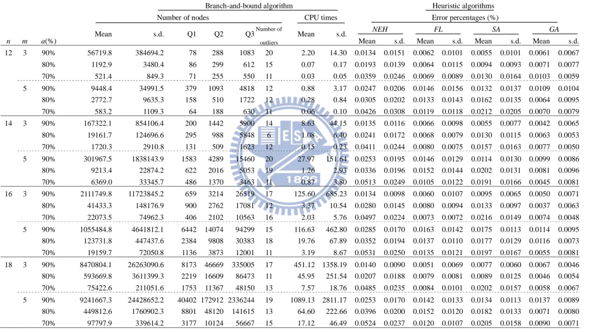
Fig 3.1. Box-plot for logarithm scale with learning effect as 70% 32

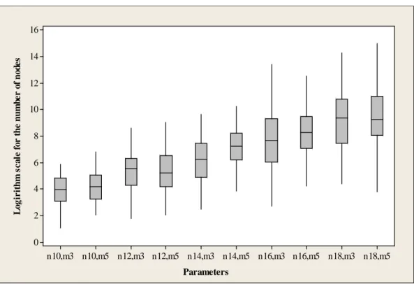
Fig 3.2. Box-plot for logarithm scale with learning effect as 80% 33

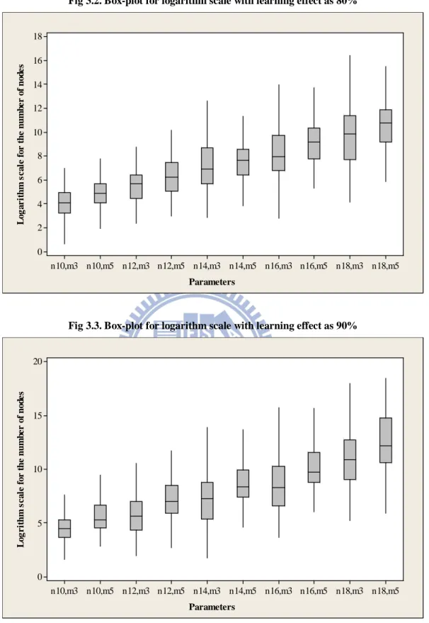
Fig 3.3. Box-plot for logarithm scale with learning effect as 90% 33

Fig 4.1. The number of nodes for branch-and-bound algorithm under different α 47

Fig 4.2. The relative percentage deviation of the learning patterns for the optimal objective value under different α 48

Chapter 1

Introduction

In manufacturing and service industries, the scheduling problem is an important field of decision-making. In a narrow sense, the meaning of scheduling is to set the priorities of tasks for optimizing certain objectives. Due to the arising of global industrialization, many researchers and practitioners devote to study the scheduling problems, and the meaning of scheduling is extended to assign limited resources to the tasks for optimizing certain objectives. The resources of scheduling problems are manpower, raw materials, and facilities and so on. In fact, an inaccurate scheduling policy may lead to crucial loss of capacity or goodwill. Since the competition of marketplace grows rapidly, an effective scheduling policy plays a critical role for making profit for an enterprise.

1.1 Research motivation

In traditional scheduling problems, it is assumed that all the job processing times are fixed and known (Pinedo [29]; Smith [32]). However, job processing times frequently decline as workers gather working knowledge and experience. For example, processing similar tasks continuously improves worker’s skills and helps them perform their jobs efficiently (Biskup [1]). This phenomenon is known as the “learning effect.” The influence of learning on productivity for aircraft industry manufacturing was first observed by Wright [44], in which the processing time of a unit declines by 20% with every redoubling output and this phenomenon is called as 80% hypothesis. Afterward, the learning effect was affirmed in numerous industries such as the manufacturing and service industries (Yelle [48]).

The phenomenon of learning in Wright [44] is presented as _{{ }} a k

p = pk ,where p{ }k denotes the actual processing time for each unit when the output requires k units, in which the

actual processing times of all units are identical; p denotes the normal processing time of a unit which is given before starting the process; and a denotes the learning index which is equal or less than zero and depended on the learning rate R. For the 80% hypothesis (i.e.

0.8

R= ), it is shown that p_{{2 }k} =0.8p_{{ }k} , and it implies that p k(2 )a =0.8pka, and then the

learning index a is derived as log 0.8₂ = −0.322. Therefore, the learning index a is set as

2

log R when the processing time of a unit decreases by 100(1−R)% with redoubling output. Subsequently, Biskup [1] applied the concept of Wright [44] and created a famous learning model by assuming every job is a unit even when the processing times are different among all jobs. Therefore, the actual processing time is based on the scheduled position of the job in the model proposed in Biskup [1].

In terms of the occurrence for the learning effect in the production activities, Biskup [2] stated that an inherent characteristic of the production environments with the learning effect is a high level of human activities, and these activities are presented as follows,

 All kinds of handicraft,

 Operating and controlling the machines,  Setting up the machines,

 Maintaining the machine,  Cleaning the machines,

 Removing the failure of the machines.

Hence, the learning effect occurs when the production activity belongs to the short-term planning. In addition, the learning effect also takes place if the production environments alter and some examples are presented as follows,

 Dealing with the jobs that have never been produced before,  Hiring new employees,

 Operating the equipments which are replaced or updated.

However, the influence of the learning should decline after a certain period of time because of the improvement for operator’s skill is limited.

The learning effect has received significant attention in scheduling field recently. In the literature with regard to the learning effect, most studies focus on single-machine setting. The discussion of flowshop scheduling problems is rarely seen. Practically, in many manufacturing and assembly facilities, numbers of operations have to be done on every job and this production environment is modeled as flowshop. Therefore, in this dissertation, we intend to study the flowshop scheduling problems with learning effects.

1.2 Literature review

Biskup [1] is a pioneer to introduce a learning model into scheduling problems in which the actual processing time of a job decreases when the job is late scheduled. He examined the problems associated with minimizing the deviation from a common due date and the sum of flow times in a single-machine environment, and demonstrated that the problems are polynomially solvable. Subsequently, numerous studies have considered this novel and extended region. Cheng et al. [6] developed a model with learning effect in which actual job processing time is based on the total normal job processing time and the position of schedule on a single machine. They then demonstrated that the makespan and total completion time problems are polynomially solvable, and demonstrated that the problems for minimizing weighted completion time and maximum lateness are polynomially solvable with certain agreeable conditions. Janiak and Rudek [16] introduced a multi-ability learning effect into a makespan single-machine scheduling problem. They established polynomial time algorithms to optimize the special cases of the problem they proposed. Furthermore, Biskup [2] presented a detailed review of scheduling problems with learning effect. Particularly, he classified the

existing models into two distinct groups: the position-based learning and the sum-of-processing-time-based learning. The position-based learning is influenced by the number of jobs processed. Meanwhile, the sum-of-processing-time-based learning considers the processing time of the jobs processed to date.

In the position-based learning model, Lee et al. [23] studied a single-machine scheduling problem with release times under learning consideration. They proposed a branch-and-bound and a heuristic algorithm to obtain the optimal and near-optimal solution for minimizing the makespan. Zhu et al. [51] studied two single-machine group scheduling problems. The job processing time is a function of job position, group position and the amount of resources assigned to the group. They verified that minimizing the weighted sum of the makespan and the total resource cost remains polynomial solvable. Furthermore, Wang et al. [39] investigated a single machine scheduling problem in which the setup time and learning effect are considered, and the setup times are past-sequence-dependent. They showed that the problems to minimize the sum of quadratic job completion time, the total waiting time, the total absolute differences in waiting time, and the sum of earliness penalties subject to no tardy jobs, are polynomially solvable. Wang et al. [37] studied a single-machine problem with learning effect and discounted cost. They showed that the shortest processing time first (SPT) rule is the optimal policy for minimizing the discounted total completion time. They then illustrated an example to demonstrate that the discounted weighted shortest processing time first (WDSPT) rule is not the optimal policy for minimizing the discounted total weighted completion time. In addition, Mosheiov and Sidney [28] developed a learning model in which the learning effects are different depend on the jobs. They formulated the makespan scheduling problem with the job-dependent learning effects as an assignment problem and conducted a Hungarian method to solve the problem. And then Koulamas [18] proved that the problem proposed by Mosheiov and Sidney [28] can be solved in O(nlogn) times under certain agreeable condition. Furthermore, Janiak and Rudek [14] proposed a new learning

effect model in which the rigorous constraints of the position-dependent approach are relaxed by assuming that each job creates a different experience for the processor. They also described the shape of the learning curve using a k-stepwise function. Hence, the diversified learning functions can be fitted by a mathematical model. Janiak and Rudek [15] proposed a new experience-based learning model where the job processing times are described by “S”-shaped functions and are dependent on the experience of the processor. They demonstrated that the makespan problem on a single processor is NP-hard or strongly NP-hard, and then provided a number of polynomially solvable cases. In addition, Huang et al. [13] investigated two resources constrained single-machine group scheduling problems in which the learning effect and deteriorating jobs are considered simultaneously. They proposed polynomial solutions under certain constraints to minimize the makespan and the resource consumption, respectively. Lee and Lai [20] considered both the effect of learning and deterioration in a scheduling model. The actual job processing time is a function on the processing times of scheduled jobs and its position in the schedule. They showed that some single-machine scheduling problems remain polynomial solvable. Toksari [33] addressed a single-machine scheduling problem with unequal release times for minimizing the makespan, in which the learning effect and the deteriorating jobs are concurrently considered. Several dominance criteria and the lower bounds are established to facilitate the branch-and-bound algorithm for deriving the optimal solution. Furthermore, Eren and Guner [9] studied a bi-criteria scheduling problem with a learning effect in an m-identical parallel machine environment, and the objective function is to minimize the weighted sum of the total completion time and total tardiness. They constructed a mathematical programming model to solve the problem. Toksari and Guner [34] considered a parallel machine earliness/tardiness scheduling problem involving different penalties under the effect of position-based learning and deterioration, and demonstrated that the optimal sequence is a V-shaped schedule under

As for the sum-of-processing-time-based learning model, Koulamas and Kyparisis [17] pointed out that employees learn more when executing jobs with a longer processing time. They introduced a sum-of-job-processing-time-based learning effect scheduling model and demonstrated that the makespan and the total completion time problems for the single machine and two-machine flowshop with ordered job processing times are polynomially solvable. Wu et al. [45] studied a total weighted completion time problem on a single machine with learning effect and ready times. A branch-and-bound algorithm was proposed to derive the optimal sequence, and the simulated annealing algorithm was implemented to obtain the near-optimal sequence. Furthermore, Cheng et al. [5] introduced a learning effect model on a single machine in which the actual job processing time is derived from the sum of the logarithm of the processing times of jobs already processed, and they show that the makespan and total completion time problems are polynomially solvable. Cheng et al. [4] proposed a two-agent scheduling problem with a truncated sum-of-processing-time-based learning effect on a single machine. A branch-and-bound algorithm was utilized to obtain the optimal solution for minimizing the total weighted completion time for the jobs of the first agent subject to no tardy job of the second agent. Wang [38] introduced an exponential sum-of-actual-processing-time-based learning effect into a single-machine scheduling problem. The special cases of the total weighted completion time problem and the maximum lateness problem are proved to be polynomial solvable under an adequate condition. Additionally, Wang et al. [41] demonstrated that, even with the effects of learning and deterioration on job processing times, the single-machine makespan problem remains polynomially solvable. Wang et al. [40] considered the weighted sum of completion times and the maximum lateness problem with the effect of learning and deterioration on a single machine where job processing times are defined as functions of their starting times and sequential positions.

have been discussed simultaneously. Yin et al. [49] examined some single-machine and m-machine flowhop problems with learning considerations where the learning effect is not only a function of the total normal processing times of jobs already processed, but also of the scheduled job position. Lee and Wu [22] presented a learning model that simultaneously combines the position-based learning and sum-of-processing-time-based learning models. They then demonstrated that the single-machine makespan and the total completion time problems are polynomially solvable, and provided polynomial-time optimal sequences for minimizing the makespan and total completion time under certain conditions in a flowshop environment. Furthermore, Wang and Li [35] studied a single machine scheduling problem with past-sequence dependent setup times in which the position-based and time-dependent learning effects are simultaneously considered. They proved that the makespan, total completion time and total lateness problems can be solved by the smallest processing time first (SPT) rule. Lai and Lee [19] addressed a general scheduling model in which the position-based and the sum-of-processing-time-based learning effects are concurrently considered. They showed that most of the models in the literatures are special cases of the model they proposed.

The concept of learning effect in a flowshop environment has been relatively neglected. However, Wu et al. [47] studied the maximum tardiness problem with the position-based learning effect in a two-machine flowshop environment. They implemented a branch-and-bound algorithm to obtain the optimal sequence, and a simulated annealing algorithm to obtain the near-optimal sequence. Li et al. [25] discussed a two-machine flowshop scheduling problem with a truncated learning effect which considers the position of the job in a schedule and the control parameter. Then the branch-and-bound and three simulated annealing algorithms were conducted to seek the optimal and near-optimal solutions. In addition, Lee and Wu [21] considered a two-machine flowshop problem with

several dominance properties to construct a branch-and-bound algorithm to obtain the optimal sequence, and established a heuristic algorithm to obtain the near-optimal sequence. Chen et al. [3] considered a bi-criteria two-machine flowshop scheduling problem with the position-based learning effect when the goal is to minimize both the total completion time and the maximum tardiness. They proposed a branch-and-bound algorithm and two heuristic algorithms to obtain the optimal and near-optimal sequences. Furthermore, Wang and Xia [42] studied flowshop problems with learning effect. They gave the worst-case bound of the shortest processing time first (SPT) algorithm for the makespan and the total flow time problems, then illustrated examples to show that the Johnson’s rule is not optimal for the makespan problem in a two-machine environment with learning consideration. Eventually, they demonstrated that two special cases remained polynomially solvable for the makespan and total completion time problems. Additionally, Wu and Lee [46] investigated a flowshop problem with learning considerations to minimize the total completion time. They implemented a branch-and-bound algorithm and heuristic algorithms to seek the optimal and near-optimal sequences, respectively.

Because of obtaining optimal sequences in scheduling problems within a flowshop environment is usually complicated, numerous works have focused on identifying efficient near-optimal sequences. Nawaz et al. [27] considered an m-machine flowshop problem for minimizing the makespan, and claimed that jobs with larger total normal processing time should be prioritized over jobs with smaller total normal processing times. They demonstrated that their proposed algorithm performs particularly well on large job-sized problems. Afterward, Liu and Ong [26] and Ruiz and Maroto [31] claimed that the algorithm developed by Nawaz et al. [27] is superior to other existing polynomial algorithms for the m-machine flowshop makespan problem. Furthermore, Rajendran and Ziegler [30] developed an algorithm for solving the weighted total completion time minimization problem in an m-machines flowshop environment. Their algorithm first generates m sequences by assigning

different weights to each machine. The sequence with the minimal total weighted completion time is then selected as the seed sequence, and an improvement scheme is employed. Woo and Yim [43] provided an algorithm for minimizing the mean flow time in an m-machine flowshop environment. Their algorithm selects a job among excluded jobs for insertion into the current partial sequence. Whenever a new partial schedule is constructed, their algorithm assesses all the possible sequences by inserting an unscheduled job into one of all slots in the current sequence at a time. The partial sequence with the least mean flow time is selected. In addition, Framinan and Leisten [11] considered an m-machine flowshop problem to minimize the mean flow time. They proposed an efficient constructive heuristic algorithm based on the concept of the algorithm of Nawaz et al. [27]. They further performed a general pairwise interchange movement to boost the quality of the partial sequences in all the iterations. Framinan et al. [10] presented a review and classification for the heuristic algorithms with a makespan objective. They distinguished a given constructive heuristic algorithm into three phases, which are index development, solution construction and solution improvement. Furthermore, Wang et al. [36] proposed a modified global-best harmony search algorithm to obtain the near-optimal solution for dealing with a makespan scheduling problem in a blocking permutation flowshop environment. The algorithm they proposed was demonstrated to outperform certain existing meta-heuristics. Zhang and Li [50] addressed an estimation of distribution algorithm for a flowshop scheduling problem with the objective of minimizing the total flowtime. They showed that the proposed algorithm could improve some current best solutions for Taillard benchmark instances.

1.3 Research objectives and methodologies

Two m-machine flowshop scheduling problems are proposed in this dissertation in which the models are based on Biskup [1]. The model proposed in Biskup [1] is presented as

,

a

j r j

p = p r where p_{j r,} denotes the actual processing time of job j at rth scheduled position,

j

p denotes the normal processing time of job j, and a≤0 denotes the learning index. The

decreasing level for the curve of r descends as r increases, and it conforms to the a phenomenon that the improvement of the worker’s skill is unobvious after the worker is proficient at the jobs. Therefore, the learning model proposed in Biskup [1] is reasonable and regarded as a theoretical learning model in many studies. In addition, the production environment for the model proposed in Biskup [1] could be regarded as the handicraft because of the learning effect is occurred in whole process when dealing with a job. Meanwhile, the learning model proposed in Biskup [1] might be considered as the reduced learning model for the industrial manufacturing.

In this dissertation, the types of learning effect of the two problems belong to position-based learning. Furthermore, the learning effects are identical on all machines in the first problem, and are varied on different machines in the second problem. Since the makespan and the total completion time are the objective functions that are widely used performance measures in the scheduling literature, the objective in this dissertation of the first problem is to minimize the makespan, and of the second problem is to minimize the bi-criteria function which is modeled as the weighted sum of the total completion time and the makespan.

While the number of the machines is more or equal than three, Garey et al. [12] demonstrated that the flowshop scheduling problem for minimizing the makespan without the learning effect is an NP-hard problem. In addition, the total completion time minimization problem is proved to be an NP-hard problem without considering the learning effect when the number of the machines is more or equal than two (Lenstra et al. [24]). Therefore, the makespan and the bi-criteria minimization problems in this dissertation are both NP-hard problems. Then the branch-and-bound algorithm is a feasible approach for deriving the

optimal sequence. In the literature with respect to the flowshop scheduling problems without learning effect, Chung et al. [7] studied an m-machine flowshop scheduling problem to minimize the total completion time. They proposed a brand-and-bound algorithm that incorporates a dominance property and an innovative lower bound to seek the optimal sequence. Thereafter, Chung et al. [8] modified the efficient property in Chung et al. [7] to deal with the flowshop scheduling problem for minimizing the total tardiness. Therefore, in this dissertation, a branch-and-bound algorithm is conducted to obtain the optimal sequence, in which the dominance properties are established based on the concept of Chung et al. [7].

Seeking for the optimal sequence of scheduling problems generally requires considerable computational time and memory for larger job-sized problems. Thus this dissertation also focuses on assessing the performances of efficiency when applying economical heuristic algorithms with the learning effect to solve the proposed problem. And then two well-known heuristic algorithms proposed form Nawaz et al. [27] and Framinan and Leisten [11] are adapted for obtaining the near-optimal sequence. Additionally, two meta-heuristic algorithms are also utilized to yield the near-optimal solutions which are simulated annealing and genetic algorithms. Eventually, the accuracy and the comparison for the priorities among proposed heuristic and meta-heuristic algorithms are discussed in this dissertation.

Chapter 2

Algorithms

2.1 Branch-and-bound algorithms

In this dissertation, two NP-hard problems are studied. In order to seek the optimal sequence, we conduct a branch-and-bound algorithm incorporated with a dominance property and a lower bound. In branch-and-bound algorithm, a given node indicates a sequence with scheduled jobs, and the nodes can be eliminated by verifying the dominance property or evaluating the lower bound. The dominance property is utilized to prove that the given node is dominated by another node. Furthermore, the lower bound is the underestimated value of the objective function based on the given node. Therefore, when the given node is dominated or its lower bound is larger than a known objective value, the given node and its offspring are eliminated in the branching tree. In addition, the branching procedure proposed in this dissertation adopts the depth-first search, and assigns jobs in a forward manner starting from the first position. The advantages of the depth-first search are less number of dynamic nodes and seeking the bottom node rapider to derive the feasible sequence. The detailed procedure of the proposed branch-and-bound algorithm is described as follows.

Step 1: Generate a near-optimal sequence and solution as the initial incumbent sequence

and solution by implementing the heuristic and meta-heuristic algorithms.

Step 2: Expand the branching tree from node ( , ,− −, )− to node (1, ,−, )− , then to node (1, 2, ,−, )− , and finally to node ( ,n n− 1, ,1).

Step 3: If the current node is a complete sequence, go to Step 6. Otherwise, go to Step 4. Step 4: Apply the dominance property to identify the current node. If it is a dominated node,

eliminate the node and its offspring in the branching tree, then go to Step 2. Otherwise, go to Step5.

Step 5: Evaluate the lower bound of the objective value for the current node. If the lower

bound for the current node is larger than the incumbent solution, eliminate the node and its offspring in the branching tree, then go to Step 2. Otherwise, go to Step 7.

Step 6: If the objective value of the complete sequence is smaller than the incumbent

solution, replace the incumbent sequence and solution with the sequence and solution of the current node. Otherwise, eliminate it.

Step 7: If there is no more node can be expanded, the final incumbent sequence is set as the

optimal sequence. Otherwise, go to Step 2.

Eventually, a flowchart is drawn in Fig 2.1. to illustrate the detailed procedure of the proposed branch-and-bound algorithm.

2.2 Heuristic algorithms

While the number of jobs increases, obtaining the optimal solution of an NP-hard scheduling problem is time-consuming. Therefore, many studies are devoted to develop efficient heuristic algorithms to derive the near-optimal solution. In addition, the objective functions in this dissertation consist of the makespan and the total completion time. Therefore,

NEH and FL denote the heuristic algorithms which is respectively adapted from the heuristic algorithm proposed in Nawaz et al. [27] and Framinan and Leisten [11], by considering the learning effect and adjusting the objective function. Eventually, the procedures of NEH and FL are detailed as follows.

NEH algorithm:

Step 1: Set sequence PS and US with empty set.

Step 2: Arranging the jobs in descending order of the total normal processing times (i.e.

, 1 m i j i p =

∑

for j=1, 2,,n. See subsection 3.1), and schedule the jobs into US.

Step 3: Set k =1.

Step 4: Select the first job from US into PS, and remove the job from US.

Step 5: If k =1, go to Step 4. Otherwise, generate k sequence by respectively inserting the job into each slot of PS.

Step 6: Select the sequence with the least objective value among k candidate sequences and update the sequence as PS.

Step 7: Set k= +k 1. If k≤n, go to Step 4. Otherwise, the near-optimal sequence is set as PS.

FL algorithm:

Step 1: Set sequence PS and US with empty set.

Step 2: Arranging the jobs in ascending order of the total normal processing times, and

schedule the jobs into US.

Step 3: Set k =1.

Step 4: Select the first job from US into PS, and remove the job from US.

Step 5: If k =1, go to Step 4. Otherwise, generate k sequence by respectively inserting the job into each slot of PS.

Step 6: Select the sequence with the least objective value among k candidate sequences and update the sequence as PS.

Step 7: If k<3, go to Step 8. Otherwise, generate ( 1) 2

k k−

sequences based on PS by performing pairwise interchange procedure. Then select the sequence with the least objective value and set as sequence PS′. If PS can be dominated by PS′ in terms of the objective value, replace PS with PS’.

Step 8: Set k= +k 1. If k≤n, go to Step 4. Otherwise, the near-optimal sequence is set as PS.

2.3 Meta-heuristic algorithms

Pinedo [29] stated that the heuristic algorithms of the constructive type start without a sequence and gradually construct a sequence by adding one job at a time. They usually can obtain a solution in a moment. However, the quality of the solutions obtained by the heuristic algorithms of the constructive type is improvable, especially when the priority of the jobs is difficult to estimate. The reason is that the solutions space for the heuristic algorithms of the constructive type is relatively narrow. Therefore, two meta-heuristic algorithms are implemented to obtain the near-optimal solutions because of their larger solutions spaces, which are simulated annealing and genetic algorithms. The procedure of seeking the solution by meta-heuristic algorithms is iteratively trying to improve a candidate solution in terms of a given measure of quality. The advantages of the meta-heuristic algorithms are few or no assumptions in searching process, and a larger space of candidate solutions. Eventually, two meta-heuristic algorithms proposed in this dissertation are detailed below.

Simulated Annealing (SA)

A description of the procedure in proposed simulated annealing is presented as follows. An incumbent sequence is generated at first, and then a new sequence is created based on the incumbent one by the neighborhood generation. The incumbent sequence is replaced with the new sequence when each one of two conditions occurred, that is (1) the objective value of the new sequence is smaller than that of the incumbent sequence, and (2) the acceptance probability is larger than a given value. Eventually, the process of proposed simulated annealing is stopped by the terminating condition, and then the final incumbent sequence is set as the near-optimal sequence. The elaboration of the simulated annealing proposed in this dissertation includes:

(1) Incumbent sequence: The incumbent sequence is generated randomly.

(2) Neighborhood generation: Two jobs of incumbent sequence are randomly selected and

exchanged to yield the new sequence.

(3) Acceptance probability: The probability of acceptance is yielded from an exponential

distribution, that is P accept

(

)

=exp

(

− × ∆α

)

, where α denotes the control parameter and ∆ denotes the increment of the objective value from the incumbent to the new sequence. Furthermore, the control parameter is set as k

β , where k is the number of

cumulated iterations to date and β is an experimental factor. And then we chose

65000

β =

a

fter some pretests

.

If the new sequence is larger than the incumbent one, the

new sequence is accepted when P(accept)>r, where r is a uniform random number between 0 and 1.

(4) Terminating condition: The seeking process is terminated after 500n iterations because

of the preliminary tests reveal that the objective value is steady after 500n iterations, where n is the number of jobs.

The advantage of SA is to avoid getting trapped in a local optimum. The value of β is initially set to a high level so that a neighborhood exchange happens frequently in early iterations, and the acceptance probability is gradually lowered when the k increases so that it becomes more difficult to exchange in later iterations unless a better sequence is yielded.

Genetic algorithm (GA)

In this dissertation, a genetic algorithm is utilized to yield the near-optimal solution. The basic idea of the genetic algorithm is to generate a population with some chromosomes as the parents, then implement the crossover and mutation operations to produce a new population as the offspring, and choose the chromosome with the best performance with regard to the objective value after some generations. The segments of proposed genetic algorithm are listed as follows.

(1) Encoding: The encoding method is to generate n uniform random numbers from (0, 1) as

the genes in a chromosome, in which the job order is set as the non-decreasing order of the genes. For example, the chromosome (0.23, 0.78, 0.32, 0.14) denotes a job sequence of (4, 1, 3, 2) with four jobs.

(2) Population size: The population size indicates the number of the chromosomes in a

generation. For a large population size, it is easier to obtain a better solution, but time-consuming. The population size N is set as 150 after some preliminary tests.

(3) Fitness value: The fitness values are evaluated to indicate the probabilities of selecting

the chromosomes. Since the problem is to minimize the objective value, the fitness value of a given chromosome should be a decreasing function of its objective value. Therefore, the fitness value of the chromosome is calculated as

1 N k j j f f =

∑

for k =1, 2,,N, where the f denotes the reciprocal of the objective value of the kth chromosome. _k

(4) Selection: A roulette wheel method is used in which the chromosomes with larger fitness

values have larger areas in the roulette wheel and have higher chances to be selected. The selection process is executed by spinning the roulette wheel, and only a chromosome is selected in each spin.

(5) Crossover: Crossover operation is to produce the chromosomes of offspring from the

generate two new chromosomes in offspring by utilizing one-point crossover, in which a cut point are randomly selected and the parts of these two chromosomes in parents are exchanged to generate new chromosomes. For example, two chromosomes in parents are presented as (0.53, 0.26, 0.72, 0.44, 0.69) and (0.91, 0.08, 0.37, 0.29, 0.55), and the new chromosomes are (0.53, 0.26, 0.37, 0.29, 0.55) and (0.91, 0.08, 0.72, 0.44, 0.69) if the randomly selected cut point is the second position. Furthermore, the crossover rate is chosen as 0.85 in this dissertation after some pretests.

(6) Mutation: Mutation operation is used to prevent getting trip in a local optimum. In this

dissertation, the procedure of mutation is to randomly select a gene in a given chromosome, and replace it with a random uniform number from 0 to 1. The mutation rate is set as 0.3 in this dissertation to determine whether the chromosome is mutated.

(7) Evolution: In order to maintain the superiority of the chromosomes, a part of

chromosomes with larger fitness values in parents are retained in the next generation. Meanwhile, the chromosomes with smaller fitness values in the offspring are eliminated as a consequence. Furthermore, the evolution rate is set as 0.5, which means 50% of the chromosomes in the parents are retained to the next generation.

(8) Termination: The proposed genetic algorithm is terminated after 50 generations after

some pretests.

Encode N chromosomes in parents and evaluate their

fitness values

Select two chromosomes in parents by roulette wheel

method

Crossover Retain these two

chromosomes as the offspring

Produce two chromosomes as offspring

Mutation

Modify these two chromosomes in offspring

Produce chromosomes

for N/2 times

Evaluate the fitness values of all chromosomes of the

offspring

Evolution Termination

Decode the chromosome with the largest fitness value

as the final solution Set the chromosomes of the

offspring as the parents

Yes Yes No Yes No Yes No No

Chapter 3

Makespan minimization for m-machine flowshop

scheduling problem with position-based learning effects

3.1 Notations and problem statement

The notations used throughout this chapter are summarized as follows. n : Number of jobs.

m : Number of machines.

N: Set of jobs, i.e., N ={1, 2,, }n .

i

M : ith machine, i=1, 2,,m.

,

i j

p : Normal processing time of job j on M . _i

, ,

i j r

p : Actual processing time of job j on M if placed at rth position in a sequence. _i a : Learning index with a<0.

S: Subset of N with s scheduled jobs.

U: Subset of N with n s− unscheduled jobs. σ : A partial sequence of set S.

[ ]: The symbol which signify the order of jobs in a sequence.

,[ ]( )

i r

C σ : Completion time of the job scheduled in the rth position on M in sequence _i σ .

( , ) j

G u v : Total normal processing time of job j from M to _u M , where _v u≤v, i.e.,

, ( , ) v j l j l u G u v p = =

∑

. ,[ ] i r

B : Earliest starting time at rth position on M . _i

,[ ]

i r

LB : The lower bound for a given node.

The problem formulation of the m-machine flowshop environment with learning effects is described as follows. Suppose that there are n jobs in set N, to be processed on m machines. Each job j comprises m operations O_{1 ,j},O_{2 ,j},,O_{m j,} , where O_{i j,} has to be

processed on Mi for i=1, 2,,m and j=1, 2,,n. Processing of operation Oi+1,j must

start only after the completion of O_{i j,} . Furthermore, the flowshop environment considers a

schedule in which the job sequence is identical on all the machines. The actual processing time p_{i j r, ,} of job j on M is a function that depends on its position r in the sequence, i.e., _i

, , ,

a

i j r i j

p = p r ,

where i=1, 2,...,m, j r, =1, 2,...,n.

This chapter attempts to identify a sequence for minimizing the makespan. Given n jobs in Set N, and τ denotes one complete sequence of all permutations. The objective of this chapter is to derive a sequence τ∗ such that C_{m n[ ]}(τ∗)≤C_{m n[ ]}( )τ for any sequence τ .

3.2 Dominance property

The following theorem provides a criterion for discriminating dominance relationships between two different sequences which are made up of the same job set.

Theorem 3.1: Let σ₁ and σ₂ denote two partial sequences with s jobs of set S . If

{

,[ ] 1 ,[ ] 2

}

1

max _{i s}( ) _{i s}( ) 0

i m C σ C σ

≤ ≤ − < , then σ1 dominates σ2.

Proof: Let π denote a partial sequence with n− jobs of set U, and sequence s π is

2 ( 2, )

S = σ π , respectively. Then for 1≤u≤m, we have the completion time of the job

scheduled in the nth position on M in _u S and is ₁

{

}

,[ ] 1 ,[ 1] 1 [ ] 1 ( ) max ( ) ( , ) a u n v n n v u C S C ₋ S G v u n ≤ ≤ = + × 1,[ 1]( 1) [ ]( , )1 a v n n C ₋ S G v u n

= + × for some v where ₁ 1 v≤ ≤ . ₁ u

Similarly, the completion time of the job scheduled in the nth position on M in _u S is ₂

{

}

,[ ] 2 ,[ 1] 2 [ ] 1 ( ) max ( ) ( , ) a u n v n n v u C S C ₋ S G v u n ≤ ≤ = + × 2,[ 1]( 2) [ ]( , )2 a v n n C ₋ S G v u n

= + × for some v where ₂ 1 v≤ ≤ . ₂ u

Then we have 1 ,[ ]( 2) ,[ 1]( 2) [ ]( , )1 a u n v n n C S ≥C ₋ S +G v u ×n for v₁ ≠ . v₂ Therefore, we have 1 1 ,[ ]( )1 ,[ ]( 2) ,[ 1]( )1 [ ]( , )1 ,[ 1]( 2) [ ]( , )1 a a u n u n v n n v n n C S −C S ≤_C ₋ S +G v u ×n _{ } − C ₋ S +G v u ×n _

{

,[ 1] 1 ,[ 1] 2

}

1 max _{i n} ( ) _{i n} ( ) i m C − S C − S ≤ ≤ ≤ − .

An induction argument is conducted. Then we have

{

}

,[ ]( 1) ,[ ]( 2) ₁max ,[ ]( 1) ,[ ]( 2) u n u n _{i m} i s i s C S C S C S C S ≤ ≤ − ≤ − . If

{

_{,[ ] 1 ,[ ] 2}

}

1 max _{i s} ( ) _{i s} ( ) 0 i m C S C S ≤ ≤ − < , then S dominates 1 S . 2

The proof is completed.

In order to apply the above theorem in the proposed branch-and-bound algorithm, the following property requires considering two consecutive jobs, as presented below.

Property 3.1: Let J and _x Jy denote two jobs of set S, and σs−2 denote a sequence with

2

s− jobs excluding J and _x J_y of set S. If

{

_{,[ ] 2 ,[ ] 2}

}

1

max _{i s} ( _s , _x, _y) _{i s} ( _s , _y, _x) 0 i m C σ − J J C σ − J J

≤ ≤ − <

3.3 Lower bound

For a given node in the branch-and-bound algorithm, the lower bound is designed to underestimate the objective function by utilizing the information of its unscheduled jobs, and the lower bound is less than or equal to the objective value of the optimal sequence based on the node. Consequently, when the lower bound of a given node is larger than the objective value of a known sequence, the optimal sequence based on the node is dominated by the known sequence, and the given node and its offspring are not the candidates for the optimal sequence.

In this subsection, we propose a lower bound for eliminating nodes in the branching tree, and the lower bound is evaluated using the concept developed by Chung et al. [7]. The lower bound for Chung et al. [7] is a machine-based lower bound. The main idea of their lower bound is assuming that the given machine has unit capacity and the machines behind it have infinite capacity. Hence, the procedure in Chung et al. [7] for estimating the marginal lower bound based on the given machine is to compute the earliest starting times for all remaining positions on the machine at first, and to sum up these starting times, and all the processing times of the machine, and that behind the machine for unscheduled jobs. Finally, the lower bound is determined as the maximal marginal lower bound. Instead of the total completion time, we adapt the procedure in Chung et al. [7] which estimates the earliest starting time with learning effect, when the objective is to minimize the makespan. The proposed lower bound is summarized as follows. Let pi,( )j represent the normal processing times on M , which are i

based on non-descending order of all p_{i j,} from set U for j =1, 2,n−s . i.e.,

,(1) ,(2) ,( )

i i i n s

p ≤ p ≤≤ p ₋ , where i=1, 2,,m. G₍₁₎( , )u v denotes the smallest total normal

processing time between M and _u M from set _v U. Let Ei s,[+1] denote the actual starting

1,[s 1] 1,[ ]s ( ) E ₊ =C σ and

{

}

{

}

,[ 1] ,[ 1] [ 1] ,[ ] 1 1 max max ( , 1) ( 1)a , ( ) i s u s s i s u i E ₊ E ₊ G ₊ u i s C σ ≤ ≤ − = + − × + , where i=2, 3,m.

For the first machine, the earliest starting time is the same as the actual starting time of s+1

th job (i.e. B_1,[s+1] =E_1,[s+1]). Then

{

}

2,[ 1] max 1,[ 1] 1,[ 1] ( 1) , 2,[ ]( ) a s s s s E ₊ = B ₊ + p ₊ × +s C σ

{

1,[ 1] 1,(1) 2,[ ]

}

max B _s+ p (s 1) ,a C _s ( )σ ≤ + × + .

Therefore, B_2,[s+1] is evaluated as max

{

B_1,[s+1]+p_1,(1)× +(s 1) ,a C_{2,[ ]s} ( )σ

}

. By induction, we have

{

}

{

}

,[ 1] ,[ 1] (1) ,[ ] 1 1 max max ( , 1) ( 1)a , ( ) i s u s i s u i B ₊ B ₊ G u i s C σ ≤ ≤ − = + − × + for i=2, 3,m.

Since the learning effect is considered, we have _{,[ ] ,[ 1] ,( )}

1 ( ) j a i s j i s i l l F ₊ B ₊ p s l =

= +

∑

+ . For the first

machine, the earliest starting time of nth job is the earliest completion time of (n−1)th job (i.e. B_{1,[ ]n} =F_1,[n−1]). In the context of Chung et al. [7] for unscheduled jobs, besides (s+1)th

job on the second to the final machine, the procedure of computing the earliest starting time only considers the earliest completion time on the current machine, and that immediately ahead of the machine (i.e. E_{i s j,[ + ]} =max

{

F_{i s j,[+ −1]},F_{i−1,[s j+ ]}

}

). However, it may have the contradiction that the earliest starting time on the current machine is smaller than that on the preceding machines for the third and late machine. Therefore, to overcome the contradiction, we have

{

}

{

}

,[ 1] 1,[ ] ,[ ] ,[ 1] 1,[ ] 1,[ ] 1,(1) max , , where 2 max , , , where 3, 4, , i n i n i n _a i n i n i n i F F i B F F B p n i m − − − − − −  ₌  =  + × =   .

bound in this chapter is represented as

{

{

_{,[ ] (1)}

}

_{,[ ]}

}

1

max max _{i n} ( , ) a , _{m n}

i m B G i m n F

≤ ≤ + × , and the

detailed procedure for estimating the lower bound is presented as follows.

Step 1: Set i=1, B1,[s+1] =C1,[ ]s ( )σ , and go to Step 3.

Step 2: Compute _{,[ 1]}

{

{

_{,[ 1] (1)}

}

_{,[ ]}

}

1 1 max max ( , 1) ( 1)a , ( ) i s u s i s u i B ₊ B ₊ G u i s C σ ≤ ≤ − = + − × + Step 3: Compute _{,[ ] ,[ 1] ,( )} 1 ( ) j a i s j i s i l l F ₊ B ₊ p s l = = +

∑

+ for j= − −n s 1 and n− . s

Step 4: If i=1, set B1,[ ]n =F1,[n−1] and go to Step 6. Otherwise, go to Step 5.

Step 5: If i=2, set B_{i n,[ ]} =max

{

F_{i n,[ −1]},F_{i−1,[ ]n}

}

. Otherwise, set

{

}

,[ ] max ,[ 1], 1,[ ], 1,[ ] 1,(1)

a i n i n i n i n i

B = F ₋ F₋ B₋ + p₋ ×n .

Step 6: If i<m, set i= +i 1and go to Step 2. Otherwise, go to Step 7.

Step 7: Set

{

{

_{,[ ] (1)}

}

_{,[ ]}

}

1 max max _{i n} ( , ) a , _{m n} i m LB B G i m n F ≤ ≤ = + × .

3.4 Computational results

In this section, several computational experiments are conducted to assess the performance of the branch-and-bound, the heuristic and meta-heuristic algorithms proposed in this chapter. All the algorithms are coded in Fortran 90 and run on a personal computer with 2.89 GHz AMD Athlon ™ II X4 635 Processor and 3.25GB RAM with Windows XP. The normal processing time of all operations are randomly generated from a discrete uniform distribution over 1 to 100. First of all, the influence of the learning effect is examined in Table 3.1, in which the number of jobs is fixed at 10, three different levels of the learning effect are set as 90%, 80% and 70% (which corresponds to a= −0.152 , a= −0.322 , and

0.515

a= − .), and 100 replications are randomly generated of each experimental condition. Therefore, a total of 600 instances are tested and the mean optimal makespans are recorded in Table 3.1. Furthermore, the optimal sequence derived from the proposed problem without learning effect under each instance, is used to calculate the makespan of the proposed problem and the mean makespans and the mean and maximum error percentages are listed in Table 3.1. For each instance, the error percentage of is calculated as O O 100%

O

∗ ∗

− _×

, where O denotes the value of the makespan calculated by the sequence derived without the learning effect and

O∗ denotes the optimal makespan. As shown in Table 3.1, it reveals that the influence of the learning effect is notable with regard to the mean error percentages. Additionally, the influence of the learning effect is higher with the stronger learning effect.

Table 3.1. The influence of the learning effect on optimal solution (n=10)

Use the optimal sequence which is derived without the learning effect mean optimal mean Error percentage

m a(%) makespan makespan mean max 3 90% 487.1 563.4 15.799 31.804

80% 375.1 531.0 42.506 75.273 70% 285.0 528.5 86.911 144.845

5 90% 580.5 634.5 9.447 26.843

In order to test the efficiency of the proposed property and the lower bound, a computational experiment is implemented with fixed job size at 10, two different machine sizes at 3 and 5, 100 replications, and three levels of the learning effect at 90%, 80% and 70%. The results are listed in Table 3.2, in which B_P denotes the branch-and-bound algorithm with only the property, B_L denotes the branch-and-bound algorithm with only the lower bound, and B_P+L denotes the branch-and-bound algorithm with both the property and the lower bound. In addition, the mean number of nodes and the mean execution time are recorded. Meanwhile, the mean execution time for the enumeration method is also recorded. As shown in Table 3.2, the efficiency of the property and the lower bound in the branch-and-bound algorithm are significant in terms of the mean execution time by comparison with the enumeration method. Furthermore, the lower bound is more effective than the property in terms of the mean number of nodes and the mean execution time, and the phenomenon is notable when the learning effect is stronger. However, the most efficient performance is exhibited when B_P+L is implemented in terms of the mean number of nodes and the mean execution time. Therefore, the branch-and-bound algorithm with both the property and the lower bound is recommended for the succeeding computational experiment in this chapter.

Table 3.2. The performance of the property and the lower bound for the branch-and-bound algorithm (n=10)

Number of mean nodes Mean CPU times

m a(%) B_P B_L B_P+L B_P B_L B_P+L Enumeration 3 90% 257236.9 917.7 450.4 4.234 0.031 0.017 15.504 80% 183932.9 162.6 129.6 3.083 0.007 0.006 15.421 70% 111829.0 92.7 78.2 1.949 0.005 0.004 15.379 5 90% 368537.7 945.1 771.2 10.067 0.067 0.056 25.148 80% 250310.5 350.0 310.5 6.892 0.027 0.027 25.051 70% 146816.5 134.3 122.3 4.031 0.012 0.012 24.806

We use four job sizes (n=12, 14, 16 and 18) and two different machine sizes (m＝3 and 5) to yield the optimal solution and test the accuracy of all the proposed heuristic and meta-heuristic algorithms. Furthermore, to examine the influence of the learning effect, the three levels of the learning effect are taken to be 90%, 80%, and 70%. Consequently, 24 experimental conditions are examined, and 100 replications are randomly generated for each condition. A total of 2,400 instances are generated and the results are listed in Table 3.3. The mean and the standard deviation of the number of nodes and of the execution time for the proposed branch-and-bound algorithm are recorded. In addition, the mean and standard deviation of the error percentages for the heuristic and meta-heuristic algorithms are also recorded. For each instance, the error percentage of the given heuristic algorithm is calculated as 100% V V V ∗ ∗ − _× ,

where V denotes the value of the makespan generated by the heuristic or meta-heuristic algorithm and V∗ denotes the optimal makespan obtained by the branch-and-bound algorithm.