Pergamon
Pattern Recognition, Vol. 30, No. 2, pp, 245-252, 1997 Copyright © 1997 Pattern Recognition Society. Published by Elsevier Science Ltd Printed in Great Britain. All rights reserved 0031-3203/97 $17.00+.00
P I I : S - 0 0 3 1 - 3 2 0 3 ( 9 6 ) 0 0 0 8 0 - 5
A
M A C H I N E L E A R N I N G A P P R O A C H F O R A C Q U I R I N G
D E S C R I P T I V E C L A S S I F I C A T I O N R U L E S OF S H A P E C O N T O U R S 1
JUI-CHI HSU and S H U - Y U E N HWANG*
Department of Computer Science and Information Engineering, National Chiao-Tung University, Hsinchu, Taiwan, R.O.C.
(Received 28 September 1995)
Abstract--We devise a method to generate descriptive classification rules of shape contours by using inductive learning. The classification rules are represented in the form of logic programs. We first transform input objects from pixel representation into predicate representation. The transformation consists of preprocessing, feature extraction and symbolic transformation. We then use FOIL which is an indictive logic programming system to produce classification rules. Experiments on two sets of data were performed to justify our proposed method. Copyright © 1997 Pattern Recognition Society. Published by Elsevier Science Ltd.
Shape representation Classification Inductive logic programming
Machine learning FOIL
1. INTRODUCTION
Shapes are important information for acquiring the notion of objects. M u c h research that utilizes shape information to perform tasks in computer vision has been done. For example, Hogg expressed that shapes can evoke a wide range of visual concepts relevant to describing object geometric properties. (1~ Jovanovid (2~ used shape information to classify model tanks, air- planes, helicopters, trucks and armored cars. Katzir et al. (3) utilized shape information to recognize spoons. Ueda and Suzuki (4) made use of shape information to classify sedan, hatchback and wagon cars. Ansari (5> adopted a landmark-based approach using shape in- formation to recognize wrenches, needle-nose pliers, wire cutters, and wire strippers. Medioni e t a / . (6'7) designed a system to find features hidden in shapes for pattern recognition.
One c o m m o n requirement in these works, as in most o t h e r o b j e c t r e c o g n i t i o n systems, is to construct classification rules or models that can be used to classify or compare with an input object. Without the help of domain experts, machine learning techniques have to be used to achieve this goal. In addition to works mentioned above, Comlell and Brady (s) designed a system that combines recognition and learning. The system utilizes shape information and generates a semantic network representation for an object. Hfittich and Wandres (9) devised a system to construct 2D models based on "learning by showing". Jovanovid (2) proposed a learning algorithm based on/-classifier to generate and
* Author to whom correspondence should be addressed. Tel.: 886-35-781366; fax: 886-35-724176; e-mail: syhwang@ci- se.nctu.edu.tw.
1Research supported by National Science Council, R.O.C., under grant number NSC 84-0408-E-009-014.
modify the structure of a pattern class. Fichera et al. (1°) used fuzzy logic and the I N D U C E system to learn the organs of h u m a n brains. Ueda and Suzuki (4) retained perceptually relevant features in shapes to learn shape models. These results show that machine learning techniques really help the task of recognition patterns well.
However, one drawback in existing research is that the characteristics extracted and learned by these systems are not easily understandable to humans. This is also the gap that exists between machine vision and h u m a n perception. Consider how people recognize simple objects such as screws or spoons. Features in these objects perceived by h u m a n are something like that screws always have a hat and a rectangle, and spoons have a long ladle. These characteristics can help us easily to determine what an object is, but will be missed if method in most previous research were to be used. For this reason, we devise a method that discovers knowledge from shape contours by using inductive learning techniques. The discovered knowledge is s y m b o l i c c l a s s i f i c a t i o n rules of two classes and represented in the form of logic programs. Our goal is to have the classification rules as descriptive as possible. The structure of this paper is as follows. Section 2 describes the transformation of shape contours from pixel level to symbolic representation. Section 3 de- scribes the learning procedure. Experimental results are shown in Section 4. Section 5 is the conclusion.
2. FROM PIXELS TO PREDICATES
This section describes how to transform the repre- sentation of input objects from pixel level into predicate level. We skip the image acquisition and boundary extraction steps, and assume that the input are in the 245
246 JUI-CHI HSU and SHU-YUEN HWANG
form of boundary pixels, with possible noises. The transformation consists of three steps: processing, feature extraction, and symbolic transformation. 2.1. P r e p r o c e s s i n g
The goal of preprocessing is to eliminate the effect of noises and geometric transformations, such as transla- tion and rotation, on the results of later processings. In our system, the step of preprocessing includes smooth- ing and the Hotelling transform.
The goal of smoothing is to reduce the influence of noises on contours. We employed a modified Ganssian kernel to smooth a contour. 01) The goal of the Hotelling transform (12) is to align all objects along their principal axes, so that the rotation of an object will not affect later processings. The X and Y axes in the experimental data (see Figs 4-10) are the principal axes found by the Hotelling transform.
2.2. Feature extraction
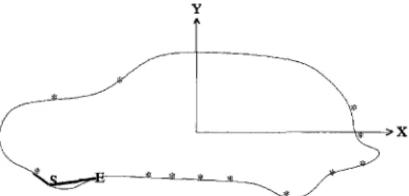
Feature extraction plays a key role in our system because it decides the information that an object can provide to the learning algorithm, and thus decides the classification rules. The first step of feature extraction is to divide the contour of a shape into segments. We employ a modified k-curvature algorithm (13) in this process. The algorithm can divide a contour by finding some segmentation points based on local curvature of segments. An " * " mark represents a segmentation point in the experimental data (see Figs 4-10).
Once the segments of a shape contour have been obtained, properties of segments are computed. The properties need to include all important characteristics of the shape, based on the segmented components. (~4) The output of this step includes three sets S i for each segment, and several AJs and P~s for entire contour, as described below. We will omit the superscripts of these sets.
S is the set that contains the information of individual segments. S = (id, loc, ht, len, con, sym). The compo- nents of S are defined below:
• id is the identification of the segment.
• Ioc indicates the location of the segment. We divide an image into four quadrants based on the axes found in the Hotelling transform. The assign numbers 0-7 indicate the different start points and end points of the segment.
• ht is the height of the segment, which the largest distance from the segment to the straight line formed by connecting the start point and the end point of the segment.
• len is the length of the segment.
• con is the number used to indicate the segment is convex or concave or straight.
• sym represents whether the segment is symmetric. A is a set which represents the interrelations between two adjacent segments. A = (id, idc, O}, as described below:
• id is the identification number of a segment. • idc is the identification number of the segment that
is clockwise adjacent to id.
• 0 is the angle between segments id and idc. P is the set which represents the possible parallelity of some segments, P = ( i d l , i d 2 , ~ ) , as described below
• idl is the identification number of a certain segment.
• id2 is the identification number of another segment. • ~b is the angle between segments idl and id2, and is
close to 0 ° or 180 °.
The set P is a d hoc compared to general information provided by S and A, which are usually referred to in literature of shape representation.
2.3. S y m b o l i c transformation
Eight types of predicates are used to represent information extracted. Type 1 links a segment with a contour. Type 2-6 correspond to S, type 6 is related to A, and type 8 is for P.
1. H a v e ( i , n ) : This means that segment n
belongs to contour i .
2. T o k e n l ( i d , l o c ): The first two elements of A are extracted to become the parameters of the predicate T o k e n 1. This predicate represents the location of segment i d . C a r 1 C a r 2 C a r 3 C a r 4 C a r 5 C a r 6 C a r 7 C a r 8 C a r N C a r 18 C m r II C a r 12
f-/f~
O a r 13 C a r 14 C a r 15 C a r 16 C a r 17 C a r 18 C a r 19 C a r 20 Car 21 Car 22A machine learning approach to acquiring descriptive classification rule 247
3.
T o k e n 2 (id. HT): T o k e n 2
is used to show whether segment i d is sharp or smooth, the parameter HT is a digitized result of ht. We assign 13 to HT if the corresponding h t is greater than the medium of the set of allhts
in S, otherwise 12 is assigned.4. T o k e n 3 ( i d , L E N ) : T o k e n 3 can deter- mine whether segment i d is narrow or wide. Similar to HT, the parameter L E N is set to 9 if the corresponding
fen
is greater than the medium of the set of alllens
in S, otherwise it is set to 8.5. T o k e n 4 ( i d , C O N ) : T o k e n 4 can show what shape of the segment i d is. CON is 15 if segment i d is concave, 16 if i d is nearly a straight line, and 17 if segment i d is convex.
6. T o k e n 5 ( i d , SYM) : T o k e n 5 can identify whether segment i d is symmetric or not. If segment i d is not symmetric, SYM is equal to 32 else SYM is equal to 33.
7.
A d j (nl ,n2, agl):
This predicate is used to represent the relationships of adjacent segments. The parameters n 1 andn 2
are formed by concatenating the digit i withid
andidc,
respectively. Whereas thethird parameter a g l is a symbolic term that is formed by first clustering all 0s into 64 groups and then for each group assigning a symbolic term. 8. P a r ( p l , p 2 , p a l ): This predicate is a sym-
bolic counterpart of P. The parameters p 1 and p 2 are formed by concatenating the digit i with
idl and
id2,
respectively. The third parameter is set to " a " if ¢ < c , and " - a " if ¢ _> 1 8 0 - e .Because we use a complete description on a shape contour, it is not surprising that a shape contour may result in a long list of predicates. For example, Fig. 2 is a symbolic representation of a car 2 in Fig. 1.
3. LEARNING SYMBOLIC CLASSIFICATION RULES As reviewed in Section l, machine techniques have been used in learning various aspects of image shapes. A theoretical analysis on learning visual concepts shows the high computational complexity in learning visual concepts in pixel level. (15) This is another reason that we intend to perform learning on symbolic level (e.g. see Fig. 2). H a v e ( 2 a , 2 a 0 ) , H a v e ( 2 a , 2 a l ) , H a v e ( 2 a , 2 a 2 ) , H a v e ( 2 a , 2 a 3 ) , H a v e ( 2 a , 2 a 4 ) , H a v e ( 2 a , 2 a 5 ) , H a v e ( 2 a , 2 a 6 ) , H a v e ( 2 a , 2 a 7 ) , H a v e ( 2 a , 2 a 8 ) , H a v e ( 2 a , 2 a 9 ) , H a v e ( 2 a , 2 a l 0 ) , H a v e ( 2 a , 2 a l l ) , H a v e ( 2 a , 2 a l 2 ) , H a v e ( 2 a , 2 a l 3 ) , H a v e ( 2 a , 2 a l 4 ) , H a v e ( 2 a , 2 a l 5 ) , H a v e ( 2 a , 2 a l 6 ) , H a v e ( 2 a , 2 a l 7 ) , T o k e n l ( 2 a 0 , 1 ) , T o k e n l ( 2 a l , 1 ) , T o k e n l ( 2 a 2 , 1 ) , T o k e n l ( 2 a 3 , 0 ) ,
Tokenl(2a4,7),
Tokenl(2a5,7),
T o k e n l ( 2 a 6 , 7 ) ,Tokenl(2a7,Y),
T o k e n l ( 2 a 8 , 6 ) , T o k e n l ( 2 a 9 , 5 ) , T o k e n l ( 2 a l 0 , 5 ) , T o k e n l ( 2 a l l , 5 ) , T o k e n l ( 2 a l 2 , 5 ) , T o k e n l ( 2 a l 3 , 4 ) ,Tokenl(2al4,3),Tokenl(2al5,3),
T o k e n l ( 2 a l t , 3 ) ,Tokenl(2al7,2),
T o k e n 2 ( 2 a 0 , 1 2 ) , T o k e n 2 ( 2 a l , 1 2 ) , T o k e n 2 ( 2 a 2 , 1 3 ) , T o k e n 2 ( 2 a 3 , 1 3 ) , T o k e n 2 ( 2 a 4 , 1 3 ) , T o k e n 2 ( 2 a 5 , 1 3 ) , T o k e n 2 ( 2 a 6 , 1 3 ) ,Token2(2a7,12),
T o k e n 2 ( 2 a 8 , 1 2 ) , T o k e n 2 ( 2 a g , 1 2 ) , T o k e n 2 ( 2 a l 0 , 1 2 ) , T o k e n 2 ( 2 a l l , 1 3 ) , T o k e n 2 ( 2 a l 2 , 1 2 ) , T o k e n 2 ( 2 a 1 3 , 1 3 ) , T o k e n 2 ( 2 a 1 4 , 1 3 ) , T o k e n 2 ( 2 a 1 5 , 1 2 ) , T o k e n 2 ( 2 a 1 6 , 1 2 ) ,Token2(2a17,12),
Token3(2a0.8). Token3(2al.8). Token3(2a2.9). Token3(2a3.9). Token3(2a4.9).
Token3(2a5.9). Token3(2a6.9). Token3(2aY.8). Token3(2a8.8). Token3(2a9.8).
Token3(2al0.9). Token3(2a11.9). Token3(2al2.8). Token3(2a13.9). Token3(2a14.9)
TokenS(2al5.8). Token3(2al6.8). Token3(2ai7.8).
Token4(2a0.1Y). Token4(2al.17). Token4(2a2.15). Token4(2a3.1Y).
Token4(2a4.15). Token4(2a5.17). Token4(2a6.15). Token4(2a7.17).
Token4(2a8.15). Token4(2ag. I7). Token4(2al0.15). Token4(2all.i7).
Token4(2a12.15). Token4(2a13.17). Token4(2al4.15). Token4(2al5.17).
Token4(2a16.17). Token4(2al7.17).
T o k e n 5 ( 2 a 0 , 3 2 ) , T o k e n 5 ( 2 a l , 3 2 ) , T o k e n S ( 2 a 2 , 3 2 ) , T o k e n 5 ( 2 a 3 , 3 2 ) , T o k e n 5 ( 2 a 4 , 3 2 ) , T o k e n 5 ( 2 a 5 , 3 2 ) , T o k e n 5 ( 2 a 6 , 3 2 ) , T o k e n 5 ( 2 a 7 , 3 3 ) , T o k e n 5 ( 2 a 8 , 3 3 ) , T o k e n 5 ( 2 a 9 , 3 3 ) , T o k e n 5 ( 2 a 1 0 , 3 2 ) , T o k e n 5 ( 2 a l l , 3 2 ) , T o k e n 5 ( 2 a 1 2 , 3 2 ) , T o k e n 5 ( 2 a 1 3 , 3 2 ) , T o k e n 5 ( 2 a 1 4 , 3 2 ) , T o k e n 5 ( 2 a 1 5 , 3 2 ) , T o k e n 5 ( 2 a 1 6 , 3 2 ) , T o k e n 5 ( 2 a l Y , 3 2 ) , A d j ( 2 a l l , 2 a l 2 , 1 a n g l ) , A d j ( 2 a Y , 2 a 8 , 1 a n g 2 ) , A d j ( 2 a 6 , 2 a Z , l a n g 3 ) ,Adj(2a5,2aZ,lang3),
P a r ( 2 a 0 , 2 a 6 , - a ) , P a r ( 2 a l , 2 a t , - a ) , P a r ( 2 a 3 , 2 a l 2 , - a ) , P a r ( 2 a 4 , 2 a 1 4 , - a ) , P a r ( 2 a 7 , 2 a g , a ) ,Par(2aZ,2alO,a), Par(2a7,2all,a),
P a r ( 2 a l 4 , 2 a 4 , - a ) .248 JUI-CHI HSU and SHU-YUEN HWANG
Recent development in machine learning has been focused on inductive logic programming (ILP), which has gained success in many domains, and is adopted in our system. We give a brief definition of ILP here. For more details please refer to reference (16). The learning agent of ILP is provided with background knowledge B, positive examples E, negative examples N, and con- strncts a hypothesis H. B, E, N, and H are logic programs. A logic program is a set of definite clauses each having the form
h ~ b l , b 2 , . . .
where h is an atom, referred to as the head of the clause, and bx, b2 . . . . is a set of atoms, referred to as the body of the clause. Usually E and N contain only ground unit- clauses with either head or body empty. The conditions for construction of H are B A H F- E and B A H F/N, that is to say, B and H together must logically imply E, but must not imply N.
Many ILP-based systems have been developed, they differ in the way to construct H. Our system employ FOIL (17) as the learning agent since it has a good performance in m a n y aspects. The system FOIL uses a top-down approach for constructing H. It constructs a rule by appending predicates to the body of the rule gradually. The selection of predicates is based on a measure of information gain.
The action of FOIL is described below.
H i s empty. Select a new head literal x to learn, and let a new Horn clause c be x.
1. Choose a literal y according to the conditions described below.
(a) y and c must contain at least one c o m m o n variable.
(b) y has the m a x i m u m information gain correspond- ing to c, i.e. it can contain the most positive examples and the least negative examples. 2. Add y into the body of c.
3. If there are still negative tuples in this new clause, go to 1, if not, add c into H.
Until H can explain all positive examples.
Once the input shapes have been transformed into the form of logic rules, they are stored in a file. FOIL can read the file and generate classification rules. M a n y a l t e r n a t i v e t e c h n i q u e s in F O I L can i m p r o v e the performance of learning. For example, we can change the type of each attribute in a predicate, the m a x i m u m variable depth, etc. We can also permit whether to find negated literals in a rule or not.
Moreover, the modification of the symbolic repre- sentation can be made to meet the need of generating more rules. For example, assume that uth contour and vth contour belong to the same class, they can be represented as S ( u ) and S ( v ) , or S ( u , v ) alone. S ( u ) means that the uth contour belongs to the S class. S ( u , v ) means that uth and vth contours are the same class S. The former representation can make FOIL run faster, but have few rules. The effect of the
latter representation is adverse. We will show this effect in our experiment.
One limitation of the FOIL system is that when more than one feature can tell positive examples from negative ones, FOIL will only extract one of them. This is because the design of FOIL is to classify two classes, but not to describe their differences. To achieve our goal for obtaining descriptive rules, we exclude those tuples which coincide with the predicates that have been learned again and again until all features are found. This will also be shown in the next section.
4. EXPERIMENTAL RESULTS
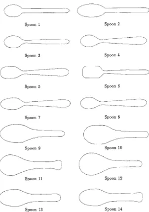
Our experiment includes two sets. The first set comprises 22 matchbox cars (see Fig. 1). These cars are divided into two classes. The second set includes 14 spoons (see Fig. 3). The first eight spoons are western style, and the rest are Chinese style spoons. Both data are further divided into a training set and a test set. In both experiments, we first used training data to learn, then used testing data to verify whether the results are correct and complete.
4.1. Experiment 1
We divided 22 cars into two classes according to the size of their wheels intuitively: cars 1-14 are classified as class 1, and the remaining cars belong to class 2. Also
Spoon 1 Spoon 2 Spoon 3 Spoon 4 f
L
,
Spoon 5 Spoon 6 Spoon 7 Spoon 8_ _ 3
i
Spoon 9 Spoon i0 ( I . _ _ j Spoon 11 Spoon 12\.
j
5
Spoon 13 Spoon 14A machine learning approach to acquiring descriptive classification ruIe 249
cars 2, 4, 6, 7, 8, 17, 19, 20, and 21 were selected as the training set, and the rest are in the testing set.
We are interested in the effect of different representa- tions on the learning result, therefore two different forms are used in our experiment. Form I represents an object using head C a r 1 ( A ) , it means that A belongs to class 1; also C a r 2 ( A ) means that A belongs to class 2. Form II uses C a r l ( A , B ) to represent that A and B b e l o n g to the same class 1, and C a r 2 ( A , B ) means that A and B belong to the same class 2.
The results using form I is shown below. Our iteration is a pass of the FOIL system. The time taken by each iteration is also shown.
i t e r a t i o n 1 ( 0 . 6 s) :
C a r 2 ( A ) : - n o t ( C a r l ( A ) ) .
C a r l ( A ) : - n o t ( C a r 2 ( A ) ) .
i t e r a t i o n 2 ( 0 . 6 s):
C a r l ( A ) : - H a v e ( A , B ) ,
T o k e n l ( B , 7 ) ,
a d j ( B , D , E ) .
i t e r a t i o n 3 ( 0 . 5 s) :
C a r l ( A ) :- H a v e (A,B) ,
a d j (B, C, l a n g l ) .
i t e r a t i o n 4
( 3 4 . 5 s) :
C a r l (A) :
- H a v e (A,B) ,
A d j (
B, C, f a n g 2 ).
After the first iteration, all predicates with form C a r 2 ( X ) were removed from all rules in training data, in order to find more classification characteristics. The rule obtained in iteration 2 indicates that one characteristic to tell class 1 from class 2 is a pair of specific segments, as shown in Fig. 4. We delete
Token(X, 7)
from training data. At the third iteration, the characteristics found are shown in Fig. 5. Similarly A d j ( X , Y , l a n g 2 ) was deleted before iteration 4. The characteristic found in the fourth iteration is shown in Fig. 6. The learning algorithm is not able to generate any rule after the fourth iteration. It is obvious that the rules generated by FOIL are consistent with our original classification based on the sizes of wheels.Y
>X
Fig. 5. One characteristic (in bold line) to classify class 1 and class 2, discovered in the third iteration of learning in form I.
Y
I > X
'\\
>
Fig. 6. One characteristic (in bold line) to classify class 1 and class 2, discovered in the fourth iteration of learning in form I.
The result based on form II is
iteration 1 (0.8s):
C a r I ( A , B ) . ' - n o t ( C a r 2 ( A , C ) ) ,
n o t ( C a r 2 ( b , C ) )
.
C a r 2 ( A , B ) : - n o t ( C a r l ( A , C ) ) ,
n o t ( C a r l ( B , C ) ) .
i t e r a t i o n 2 ( 5 6 . 7 s) :
C a r I ( A , B ) :- H a v e ( A , C ) ,
Adj (C,D,E),
H a v e (B, F) ,
A d j ( G , F , H ) .
i t e r a t i o n 3 ( 3 0 . 5 s) :
C a r 2 ( A , A ) : - H a v e ( A , C ) ,
T o k e n 2 ( C , 1 3 ) ,
T o k e n l (C,6).
i t e r a t i o n 4 ( 1 9 3 . 4 s ) •
C a r 2 ( A , B ) :- H a v e ( A , C ) ,
T o k e n 3 ( C , 9 ) ,
A d j ( C , E , 0 a n g 3 ) ,
H a v e (B,G) ,
T o k e n 2 ( G , 9 ) ,
A d j (G, I, 0 a n g 3 ) .
/
x
Fig. 4. One characteristic (in bold line) to classify class 1 and class 2, discovered in the second iteration of learning in form I.
Similarly, some predicates were taken away after each iteration in order to obtain more rules. Compared to form I, the rules obtained in the second iteration have already included all characteristics obtained using form I. The third iteration did not generate any interesting result and can be ignored. One more characteristic was found in the fourth iteration, as shown in Fig. 7. As indicated, learning using form II used m u c h more time than using form I.
250 JUI-CHI HSU and SHU-YUEN HWANG
X
f
Fig. 7. One characteristic (in bold line) to classify class 1 and class 2, discovered in the fourth iteration of learning in form II.
We then used the rules learned for classifying testing data, and the result was consistent. Another test is to perform the same learning but using the testing data. We found the consequent rules are the same as those generated by using the training data.
4.2. Experiment 2
We first split 14 spoons into a training set and a testing set. Spoons 1, 2, 3, 6, 9, 10, 14 are in the training set, and the rest are in the testing set. As in experiment 1, two forms are used in this experiment. Form I is S I ( A ) and S 2 ( A ) , while f o r m I I i s S l ( A , B ) and S 2 ( A , B ) . They have similar meanings as in Section 4.1.
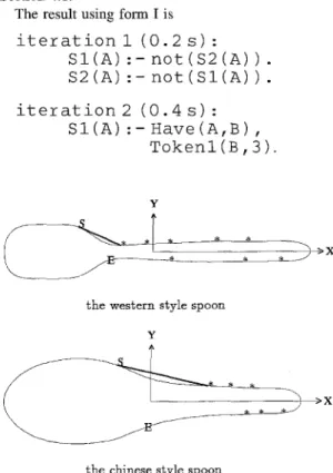
The result using form I is i t e r a t i o n i ( 0 . 2 s) : S I ( A ) :- n o t ( S 2 ( A ) ) . S 2 ( A ) :- n o t ( S l ( h ) ) . i t e r a t i o n 2 ( S I ( A ) : - 0 . 4 s ) : H a v e ( A , B ) , T o k e n l ( B , 3 ) . Y ~ > X
the western s~yle spoon
Y
>X
the chinese style spoon
Fig. 8. The corresponding features in counter of the learning result obtained in the 2ud iteration of experiment 2, form I.
After the first iteration, predicates in the form
S 2 ( X ) were taken away from all object's description. The second iteration generated a classification char- acteristic, as shown in Fig. 8.
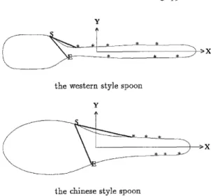
The results using form II is i t e r a t i o n 1 ( 0 . 2 s) • S I ( A , B ) :- n o t ( S 2 ( A , C ) ) , n o t ( S m ( B , C ) ) . S 2 ( A , B ) :- n o t ( S l ( A , C ) ) , n o t ( S l ( B , C ) ) . i t e r a t i o n 2 ( 9 . 0 s) - S I ( A , B ) :- H a v e ( A , C ) , T o k e n l ( C , 3 ) , H a v e ( B , E ) , T o k e n l ( E , 3) . i t e r a t i o n 3 ( 1 6 . 9 s ) : S I ( A , B ) :- H a v e ( A , C ) , T o k e n 2 ( C , 1 7 ) , A d j ( C , I , J ) , H a v e ( B , E ) , T o k e n 2 ( E , 1 7 ) , A d j ( E , G , H ) : i t e r a t i o n 4 ( 1 8 . 1 s ) : S I ( A , B ) :- H a v e ( A , C ) , H a v e ( B , D ) , T o k e n l (C, 7) ,
Adj (C,F,G),
i d j ( D , H , G ) . i t e r a t i o n 5 ( 1 7 2 s) : i t e r a t i o n 6 ( 1 9 . 7 s) : S 2 ( A , B ) .- H a v e ( A , C ) , T o k e n l ( C , 2 ) ,hdj (I,C,J),
H a v e ( B , E ) , T o k e n l (E, 2) , A d j ( G , E , H ) . i t e r a t i o n 7 ( 2 0 . 1 s ) : S 2 ( A , B ) : - H a v e ( A , C ) , H a v e ( B , D ) , T o k e n 3 ( C , 9 ) , A d j ( C , F , G ) , A d j ( D , H , G ) .S 2 ( X , Y ) was excluded from all descriptions after iteration 1. The second iteration obtained the same result as the second iteration using form I. After T o - k e n 1 ( X , 3 ) was deleted, the third iteration gener- a t e d r u l e s t h a t c o r r e s p o n d to F i g . 8, t h e n T o k e n 2 ( X , 1 7 ) was removed. The fourth itera- tion generated a rule as shown in upper spoon of Fig. 10, then T o k e n l ( X , 7 ) was deleted. Note that no rule was generated in iteration 5, so we removed one more predicate S 1 ( X , Y ), in order to obtain the description of class 2. Iteration 6 generated character- istics shown in Fig. 9, then T o k e n l ( X , 2 ) was taken away. Finally, iteration 7 generated characteristics shown in the lower spoon of Fig. 10. Similarly, much
A machine learning approach to acquiring descriptive classification rule 251
Y
~ * * , ~ _ ~ > x
the western style spoon Y
>X
the chinese style spoon
Fig. 9. The corresponding features in counter of the learning result obtained in the 3rd iteration of experiment 2, form II.
Y
~
>X
the western style spoon Y
> x
the chinese style spoon
Fig. 10. The corresponding features in counter of the learning result obtained in the 3nd and 4th iterations of experiment 2,
form II.
more time was consumed compared to the learning in form I.
We followed the same procedure used in the first experiment to check the consistency of training data and testing data. The experimental results show that the consistency exists. That is, the obtained rules using the training data are the same as those using the testing data.
5. CONCLUSIONS
Experimental results demonstrated the capability of our m e t h o d on k n o w l e d g e extraction f r o m shape contours. The generated rules reflect the properties of contours that tell one class from the other, and are easily understandable to humans. Our approach is rotation invariant and noisy resistant. Using the principal axes transform makes contours located in a consistent co- ordinates, no matter how contours rotate. The smoothing method eliminates the effect of noisy data.
Limitation of our approach are discussed below. First, our method is not scale invariant. Second, if the features used to discriminate different classes of objects are only small sharp protrusions or indentations on contours, these features m i g h t be filtered by the smoothing method. Third, the kScurvature algorithm may not segment the curvature faithfully. Lastly, while using FOIL to learn, we have to assign some parameters to FOIL. These parameters can change the type of each attribute in a predicate, the m a x i m u m variable depth, the appearance of a negated literal, the m i n i m u m accuracy of any rule, e t c . In FOIL learning, these parameters affect performance greatly. The values of these parameters are assigned basing on our present experience.
R E F E R E N C E S
1. D.S. Hogg, Shape in machine vision, Image and Vision Computing 6(11), 309-316 (1993).
2. L. Jovanovid, Learning algorithm based on modified structure of pattern classes, Proc. l l t h IAPR Int. Conf. Pattern Recognition, 487-490, (1992).
3. N. Katzir, M. Lindenbaum and M. Porat, Curve segmentation under partial occlusion, IEEE Trans. Pattern Anal. Mach. Intell. PAMI 16(5), 513-519 (1994). 4. N. Ueda and S. Suzuki, Learning visual models from
shape contours using multiscale convex/concave structure matching, 1EEE Trans. Pattern Anal. Mach. lntell. PAMI 14(4), 337-352 (1993).
5. N. Ansari, Shape recognition: A landmark-based approach, UMI Dissertation Services (1988).
6. P. Saint-Marc, H. Rom and G. Medioni, B-spline contour representation and symmetry detection, IEEE Trans. Pattern Anal Mach. Intell. PAMI 15(11), 1191-1197 (1993).
7. H. Rom and G. Medioni, Hierarchical decomposition and axial shape decomposition, IEEE Trans. Pattern Anal. Mach. Intell. PAMI 15(10), 973-981 (1993).
8. J.H. Connel and M. Brady, Generating and generalizing models of visual objects, Artificial Intell. 3, 159-183 (1987).
9. H~ittich, W. H. Wandres, Automatic learning of structural models for workpiece recognition systems, IEEE Trans. Pattern Anal. Mach. Intell. PAMI 12(3), 279-281 (1990). 10. O. Fichera, R Pellegretti, E Roli and S. B. Serpico,
Automatic acquisition of visual models for image recogni- tion, Proc. l l t h IAPR Int. Conf. Pattern Recognition, 95-99 (September 1992).
1l. E Mokhtarian and A. Mackworth, Scale-based description and recognition of planar curves and two- dimensional shapes, IEEE Trans. Pattern Anal. Mach. Intell. PAMI 8(1), 34-43 (1986).
12. R. C. Gonzalez and R. E. Woods, Digital Image Processing, Addison-Wesley, Reading, MA (1992). 13. A. Rosenfeld and E. Johnston, Angle detection on digital
curves, IEEE Trans. Computers 22, 875-878 (1973). 14. E. Sannd, Identifying salient circular arcs on curves,
Computer Vision Graphics Image Process. 58(3), 327-337 (1993).
15. H. Shvaytser, Learnable and nonlearnable visual concepts, IEEE Trans. Pattern Anal. Mach. Intell. PAMI 12(5), 459-466 (1990).
16. S. Muggleton, Inductive logic programming: derivations, successes and shortcomings, SIGART Bulletin 5(1), 5-11 (1994).
17. R.M. Cameron-Jones and J. R. Quinlan, Efficient top- down induction of logic programs, SIGART Bulletin 5(1), 33-42 (1994).
252 JUI-CHI HSU and SHU-YUEN HWANG
A b o u t the A u t h o r - - J U I - C H I HSU received a B.S. from Department of Computer Science and Information Engineering, National Taiwan University in 1990, an M.S. from the Department of Computer Science and Information Engineering, National Chiao Tung University in 1995. His research interests include Pattern Recognition and Machine Learning.
A b o u t the A u t h o r - - SHU-YUEN HWANG is a Professor in the Department of Computer Science and Information Engineering, National Chiao Tung University. He received B.S. and M.S. degrees in Electrical Engineering from National Taiwan University in 1981 and 1983; and a Ph.D. degree in Computer Science from the University of Washington in 1989. His current research interests include Artificial Intelligence, Computer Simulation and Mobile Computing.