A Reconfigurable Formation and Disjoint Hierarchical Routing for Rechargeable Bluetooth Networks

energies

A Reconfigurable Formation and Disjoint Hierarchical

Routing for Rechargeable Bluetooth Networks

Chih-Min Yu1,* and Yi-Hsiu Lee2

1 _{Department of Electronics Engineering, Chung Hua University, Hsinchu 300, Taiwan}

2 _{The Institute of Communication Engineering, National Chiao Tung University, Hsinchu 300, Taiwan;}

cmmint0160225.cm01g@nctu.edu.tw

* Correspondence: ycm@chu.edu.tw; Tel.: +886-3-5186034 Academic Editor: Hongjian Sun

Received: 16 March 2016; Accepted: 27 April 2016; Published: 5 May 2016

Abstract:In this paper, a reconfigurable mesh-tree with a disjoint hierarchical routing protocol for the Bluetooth sensor network is proposed. First, a designated root constructs a tree-shaped subnet and propagates parameters k and c in its downstream direction to determine new roots. Each new root asks its upstream master to start a return connection to convert the first tree-shaped subnet into a mesh-shaped subnet. At the same time, each new root repeats the same procedure as the designated root to build its own tree-shaped subnet, until the whole scatternet is formed. As a result, the reconfigurable mesh-tree constructs a mesh-shaped topology in one densely covered area that is extended by tree-shaped topology to other sparsely covered areas. To locate the optimum k layer for various sizes of networks, a peak-search method is introduced in the designated root to determine the optimum mesh-tree configuration. In addition, the reconfigurable mesh-tree can dynamically compute the optimum layer k when the size of the network changes in the topology maintenance phase. In order to deliver packets over the mesh-tree networks, a disjoint hierarchical routing protocol is designed during the scatternet formation phase to efficiently forward packets in-between the mesh-subnet and the tree-subnet. To achieve the energy balance design, two equal disjoint paths are generated, allowing each node to alleviate network congestion, since most traffic occurs at the mesh-subnet. Simulation results show that the joint reconfigurable method and routing algorithm generate an efficient scatternet configuration by achieving better scatternet and routing performance than BlueHRT (bluetooth hybrid ring tree). Furthermore, the disjoint routing with rechargeable battery strategy effectively improves network lifetime and demonstrates better energy efficiency than conventional routing methods.

Keywords:bluetooth; scatternet formation; topology configuration; routing; energy harvesting

1. Introduction

Bluetooth [1] communication is a valuable technology for the formation and operation of short-range wireless ad hoc networks. This technology enables the design of low-power, low-cost and short-range radio [2] that can be embedded in existing portable devices. Initially, Bluetooth technology was designed as a cable replacement solution for portable and fixed electronic devices. As mobile devices like mobile phones, personal digital assistants (PDA), digital cameras and laptop computers have grown in popularity, there has been a similarly growing demand for the ability to connect these devices into networks. Thus, Bluetooth is an ideal candidate for the construction of wireless sensor networks [3].

The Bluetooth-based sensor network faces a number of problems, however, including methods of device discovery for a node to participate in multiple piconets, and the scatternet formation algorithm, which aims to construct individual piconets and connect them into a scatternet. A Bluetooth scatternet

can be used in several applications, such as home networking, environment monitoring and sensor or ad hoc networks.

With centralized infrastructures, many message delivery services are distributed via active Internet connection. Using smartphone applications, individual users can conduct packet transmissions to interested users over Bluetooth ad hoc wireless connections, while methods for sharing information over delay-tolerant networks (DTN) are being developed [4] in order to achieve social routing over Bluetooth low energy (BLE) multi-hop scatternets. Increasingly, many BLE data applications are emerging in our daily lives, such as personal area networks, body area networks, sensor networks, etc. However, these applications pose some important research challenges, such as connecting BLE devices to share information between users, and forming the desired network configurations for various types of network applications.

Bluetooth wireless technology makes it possible to transmit time-constraint video/audio in mobile and pervasive environments. Most wireless sensor network (WSN) applications are event-driven. The main WSN architecture has a multi-level network topology with a large number of sensor nodes deployed within a geographic area, often communicating to an external network through a gateway node. The information communication between the sensor nodes and the gateway node is a multi-hop architecture to extend the network coverage. Typical WSN applications with such Bluetooth topology include: video streaming transmission [5], health monitoring [6] and data collection [7]. However, the performance of WSNs is constrained by limited battery capacity. To date, several approaches have been introduced to reduce the energy consumption and correspondingly maximize the lifetime of WSNs, such as data aggregation, green routing and sleep scheduling mechanisms. Among them, energy harvesting (EH) technology [8] is very promising, due to the unlimited energy supply provided by power sources such as solar power.

Therefore, in order to efficiently forward packets and manage harvesting energy for a rechargeable Bluetooth sensor network, this study proposes a reconfigurable mesh-tree with a disjoint hierarchical routing protocol. In contrast to our prior work [9], the size of the mesh-subnet is fixed and predefined by the constant k value regardless of the network size. However, the reconfigurable mesh-tree determines the variant k instead of the constant k layer in the mesh-subnet for the various sizes of networks. In addition, the reconfigurable mesh-tree can dynamically compute the optimum layer k when the size of the network changes in the topology maintenance phase. As a result, the reconfigurable mesh-tree constructs a desired mesh-shaped topology in one densely covered area that is extended by several tree-shaped topologies to other sparsely covered areas.

Thus far, most scatternet formation methods partition networks by collecting complete topology information [10–12], thereby introducing considerable computation or communication overheads. To mitigate topology formation overhead, a peak-search method is proposed with partial topology information. The peak-search method designs three blocks: the connection link, the hop length and the optimum decision blocks. The connection link block calculates the total number of links, the hop length block computes the average query hop and the optimum decision block uses a decision-making criterion to locate the desired k layer for the mesh-subnet.

With the packet forwarding in the mesh-tree topology, most of the sensor traffic loads pass through the mesh-subnet to the sink node. From the energy consumption point of view, the nodes nearer the sink forward most of the packets, and deplete their batteries more rapidly than other nodes, and thus become an energy hole in a network. To balance the traffic load and mitigate the energy hole problem in the mesh-subnet, two equal disjoint paths are designed for each node forwarding packets to the sink. The design goal of the routing algorithm is to balance the energy consumption for hot-spot nodes, and to deliver packets from one subnet to all other subnets effectively. Thus, by simultaneously harvesting renewable energy, the network lifetime of the hot-spot nodes can be prolonged by the two equal paths routing design.

The remainder of this paper is arranged as follows: Section2reviews current Bluetooth scatternet formation and routing protocols. In Section3, the reconfigurable mesh-tree concept and the formation

algorithm are presented. In Section4, the peak-search method to achieve the desired configuration is described in detail. In Section5, the hierarchical routing protocol for the reconfigurable mesh-tree topology is presented. In Section6, computer simulations are used to demonstrate the scatternet, routing and energy performances. Finally, conclusions are offered in Section7.

2. Related Work

Many scatternet formation algorithms have been developed for the construction of multi-hop sensor networks. These algorithms can be divided into two categories. The first [13–17] deals with situations in which all nodes are within radio range. The second category [18–23] deals with situations in which all nodes are not necessarily within radio range. Depending on the purpose of a scatternet, a number of different topology models [24] can be generated. These scatternet topology models can be generally categorized as tree-based, ring-based or mesh-based topologies, although bus and star topologies have also been studied.

Tree scatternet formation (TSF) [13] is a simple algorithm used to generate a tree topology. Initially, each node alternately switches between inquiry and inquiry-scan mode to find its neighbor nodes. Then the root node connects with neighbor nodes in the piconet formation phase. In addition, two sub-trees can be merged via the roots, and the master node becomes the new root of the merged tree topology. In [14], all Bluetooth devices are classified as components. A component can be a node, a piconet or a scatternet. Initially, all nodes are leader nodes, connecting with other nodes. When a link is established, the master node will become the leader of this component. This leader will then try to connect with other components. Finally, all components will be connected, and a large tree-shaped scatternet is generated.

In [15], a node which has complete knowledge of all other nodes is elected as the leader of the scatternet. This leader then partitions the entire scatternet topology by optimizing the number of piconets according to a predefined formula. In [16], a super master collects all nodes’ information, distributes the role for each node, and controls the topology shapes into line, bus, star or mesh by their corresponding parameters.

A Bluetooth hybrid ring tree topology called BlueHRT (bluetooth hybrid ring tree) [17] has been proposed for operation with a non-uniform distribution of Bluetooth devices. The protocol forms a ring topology in densely covered areas, which is connected with multiple tree subnets around sparsely covered areas. BlueHRT aims to mitigate the bottleneck problem in dense areas for high traffic loads, while reducing the path length in terms of delays among devices in the surrounding areas. Three-phase algorithms are designed to form a hybrid ring-tree scatternet, including discovery, role assignment and connection algorithms. During the inquiry phase, a discovery algorithm compares the addresses of all Bluetooth devices and selects the root with the largest number of addresses as a leader. In the role-assignment algorithm, the root assigns master nodes and slave/slave bridges in the ring area, as well as master/slave nodes for the tree topology. In the connection phase, all master and master/slave nodes start to page their slaves and connect the scatternet to a hybrid ring-tree topology.

Bluetree [18] is the first scatternet formation protocol to build a tree hierarchy (TH) for Bluetooth ad hoc networks. It adopts one or several root nodes to start the formation of a scatternet. The resulting topology is tree-shaped, and uses master/slave nodes to serve as relays throughout the entire scatternet. Although its spanning tree architecture achieves a minimum number of connection links between any two nodes, its tree-shaped topology is not reliable under dynamic topological changes [19]. In addition, while the algorithm is easily implemented, the root node is likely to become a bottleneck.

Bluenet [20] and Bluestar [21,22] are good examples of master/slave mesh (MSM) topology. Bluenet sets up a scatternet in a distributed manner, and the mesh-like architecture is able to achieve higher information-carrying capacity than can a tree-shaped architecture. In Bluestar, each node initially executes an inquiry procedure in a distributed manner to discover its neighboring devices, then a number of masters are selected based on the number of their neighbors. Finally, a number of gateways are selected by these masters, and thus, a mesh-like scatternet is formed. The MSM

model may use master/slave or slave/slave nodes as relays to increase scatternet performance with additional protocol complexity.

In [23], a practical formation algorithm is used to build a large tree scatternet application for solar energy farms. Based on a piconet structure, the tree hierarchy is generated from a root node to the leaf nodes via master–slave links. An asymmetrical merging procedure is iterated to merge sub-trees, or to reduce depth by an active node until a scatternet is formed. This network is developed for application in the collectors in large solar energy farms.

In order to achieve path length reduction, a hybrid mesh-tree (HMT) formation method is proposed in [9]. This method uses a designated root to propagate constant k in its downstream direction in order to construct a mesh-shaped topology and determine new roots for its descendant tree-hierarchical nodes. Each new root then starts to build its own tree subnet until the entire scatternet is formed. As a result, the mesh–subnet size can be controlled by the appropriate selection of the k parameter.

Notably, routing protocol design is another leading research field for Bluetooth multi-hop scatternets. Thus far, many well-known routing protocols have been presented, including proactive, reactive and hybrid methods, for Bluetooth networks. In the proactive category [18], each master manages a routing table, such as its downstream nodes in the spanning tree architecture. Although this involves a small delay in determining a route, the routing information periodically exchanges to generate network overhead; this is the main challenge involved in this method. Usually, a flooding or broadcasting method is used to search for the optimal path from a source node to a destination node in the reactive category [25,26]. As a result, the reactive approach incurs a certain amount of packet overhead in terms of packet delay for path discovery, but provides better network scalability. In the hybrid category [27,28] of Bluetooth scatternets, the performance of a hybrid routing protocol is simulated, and a trade-off between routing overhead, route discovery latency and the amount of storage occurs.

3. Mesh-Tree Topology Design

A simple application of the reconfigurable mesh-tree is a network consisting of one designated root as a sink node with master or relay nodes in the mesh subnet, and several new roots, with their connected nodes, in the tree subnet. With the mesh subnet in a densely covered area, the path length of the network can be reduced to less than that of a ring topology, and the traffic load of the root node can also be mitigated to less than that of a tree topology.

The reconfigurable mesh-tree assumes that a set of Bluetooth nodes is randomly distributed in a specific geographical area, and not all nodes are necessarily within radio range. In order to construct a multi-hop scatternet, two additional assumptions are made: (1) Every node is aware of the number and the identity of its one-hop neighbors upon completing the boot procedure; (2) There is at least one path between any two nodes in the network.

In contrast to our prior work [9], the size of the mesh-subnet is fixed and predefined by the constant k value regardless of the network size. However, the reconfigurable mesh-tree determines the variant k instead of the constant k layer in the mesh-subnet for the various network sizes.

3.1. Scatternet Formation

With a new root selection process, the designated root sets constant k and c as parameters. Where k is the number of layers and c is designed as a counter of the hop length from each downstream master to the designated root. With k = I = 2 and c = 0, the first root initially propagates these two parameters in the downstream direction and pages up to seven neighboring slaves to form a piconet. Each slave then switches its role to master (called an M/S node) and pages additional slaves. These new masters increase c by one, decrease k by one and continue to propagate the k parameter in the downstream direction.

After this, the new masters begin to page up to seven neighboring slaves and connect their slaves to form their own piconets. Finally, each new master will switch to return mode and wait for the return signal notification.

In this method, when the kth master is reached, k = 0. The master becomes a new root, and the k propagation process stops. The root selection process continues until all new roots are selected. The tree-shaped subnet of the designated root is thus created. At the same time, each new root repeats the same procedure as the designated root to build its own tree-shaped subnet, until the whole scatternet is formed.

After each new root is determined, it notifies its upstream masters to start a return connection procedure. During the return connection phase, a new parameter, r, is also added to represent the number of return links of each M/S node. When each returning master alternately switches its state between page and page-scan activities to connect with additional M/S nodes, the parameter r can be increased by one. Finally, each return master will pass its node ID (identification), c and r to the designated root when each master finishes the return connection phase.

This procedure is run iteratively until the designated root is reached. As a result, the tree-shaped subnet of the designated root is converted into a mesh-shaped subnet. In addition, the root node collects sufficient information to calculate the average query path length, the total number of nodes, and the total number of return links for the optimum peak-search method decision. The peak-search method is described in detail in Section4.1.

When the optimum, I, is not located, the root node propagates these two parameters with k = I + 1 and c = 0 in the downstream direction to increase the tree-shaped subnet by one more layer, as well as to generate new masters. During the return connection, only the new masters can connect with their neighboring M/S nodes and increase the return link parameter r. This procedure is repeated until the optimum I is determined. When the M/S node cannot connect with its downstream master, it will reset parameter r = 0 and send its ID to the root node to cancel the return connection.

In the topology maintenance phase, the optimum layer I can be increased or decreased by executing the reconfigurable method again when the size of the network becomes larger or smaller than a predefined threshold value.

Energies 2016, 9, 338 6 of 18

R Root Master/Slave

Connection formed in the return connection process

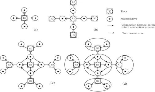
R2 (a) (b) R2 R2 R2 R2 R2 R2 R2 R2 R2 R2 R2 (c) _(d) R1 R1 R1 R1 Tree connection

Figure 1. Scatternet formation process of a reconfigurable mesh-tree. (a) The designated root R1

connects with the first tier masters. (b) When the second tier masters R2 are reached and the counter limit k = 0, these masters become new roots. (c) These new roots request their upstream masters to start the return connection procedure until R1 is reached. (d) The mesh-shaped topology of the designated root is formed and each new root manages its own tree-shaped subnet. R1, the designated root; R2, the second tier masters.

These new roots request their upstream masters to start the return connection procedure until R1 is reached. The topology of the designated root is completed, and generates a mesh-shaped subnet. At the same time, these new roots start to page new slaves and connect with their immediate downstream masters (leaves in this example), as shown in Figure 1c, to build their own tree-shaped subnets. Finally, the mesh-shaped topology of the designated root is formed and each new root manages its own tree-shaped subnet, as shown in Figure 1d.

3.2. Scatternet Performance

In the scatternet performance simulation, it was assumed that Bluetooth nodes were randomly located within a rectangular area of 40 × 40 m2_{, while a radio transmission range of 10 m was}

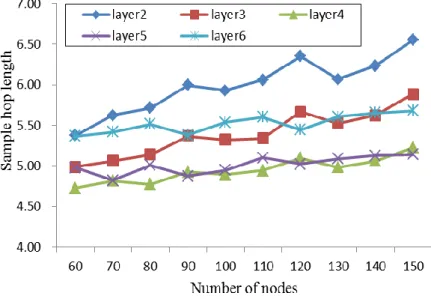
assumed. The number of simulated nodes ranged from 60 to 150. As shown in Figure 2, the k = 4 case almost achieves the lowest hop length of a sample topology, while the k = 5 case achieves a performance similar to the k = 4 case. However, the k = 6 case generates a poorer performance than that of the k = 5 case, as some tree branches did not satisfy the criterion to execute the return connection mechanism, even with the largest k. In addition, the difference between the lowest hop length and the highest hop length increases as the number of nodes increases. As a result, the lowest average hop length is either the fourth or fifth case for various sizes of network; both cases improved in hop length by approximately 20% more than the k = 2 case through averaging the sample hop length for various numbers of nodes. In addition, the improvement ratio of the hop length increases as the number of nodes increases.

To determine the optimal k layer with the lowest hop length for various topologies, it is essential for a root node to collect all scatternet topology information of various k layers. For the 100-node topology example, a root node forms a mesh-tree scatternet with k = 2, k = 3, k = 4, and up to k = 5 cases. The root node then computes the average hop length of these four cases and determines that k = 4 is the optimal layer with the shortest hop length. However, the optimal layer k is an NP (nondeterministic polynomial) complete problem, since the root node can only acquire the

Figure 1. Scatternet formation process of a reconfigurable mesh-tree. (a) The designated root R1 connects with the first tier masters. (b) When the second tier masters R2 are reached and the counter limit k = 0, these masters become new roots. (c) These new roots request their upstream masters to start the return connection procedure until R1 is reached. (d) The mesh-shaped topology of the designated root is formed and each new root manages its own tree-shaped subnet. R1, the designated root; R2, the second tier masters.

Here, k = 2 is used in Figure1as an example to describe the reconfigurable mesh-tree scatternet formation process. Initially, the designated root R1 connects with the first tier masters, as shown in Figure1a. Then, the first tier masters decrease k by one, and continue to connect with their downstream masters. When the second tier masters are reached and the counter limit k = 0, these masters become new roots, as shown in Figure1b. The tree-shaped subnet of the designated root is thus created.

These new roots request their upstream masters to start the return connection procedure until R1 is reached. The topology of the designated root is completed, and generates a mesh-shaped subnet. At the same time, these new roots start to page new slaves and connect with their immediate downstream masters (leaves in this example), as shown in Figure1c, to build their own tree-shaped subnets. Finally, the mesh-shaped topology of the designated root is formed and each new root manages its own tree-shaped subnet, as shown in Figure1d.

3.2. Scatternet Performance

In the scatternet performance simulation, it was assumed that Bluetooth nodes were randomly located within a rectangular area of 40 ˆ 40 m2, while a radio transmission range of 10 m was assumed. The number of simulated nodes ranged from 60 to 150. As shown in Figure2, the k = 4 case almost achieves the lowest hop length of a sample topology, while the k = 5 case achieves a performance similar to the k = 4 case. However, the k = 6 case generates a poorer performance than that of the k = 5 case, as some tree branches did not satisfy the criterion to execute the return connection mechanism, even with the largest k. In addition, the difference between the lowest hop length and the highest hop length increases as the number of nodes increases. As a result, the lowest average hop length is either the fourth or fifth case for various sizes of network; both cases improved in hop length by approximately 20% more than the k = 2 case through averaging the sample hop length for various numbers of nodes. In addition, the improvement ratio of the hop length increases as the number of nodes increases.

Energies 2016, 9, 338 7 of 18

formation topology of its own k layer case instead of all other cases. As a result, the design goal of a reconfigurable mesh-tree algorithm attempts to determine the optimum layer k in terms of the mesh-subnet size with lower communication and computation overheads. In addition, the reconfigurable mesh-tree can dynamically compute the optimum layer k when the size of the network changes in the topology maintenance phase.

Figure 2. Average path length in a scatternet.

4. Reconfiguration Formation Algorithm

After scatternet formation, the root node acquires the k-1 layer topology information instead of the complete topology of all layers. To realize and decide the optimum layer k with partial scatternet topology knowledge in the root node, a heuristic algorithm called the peak-search method is proposed in order to achieve the lowest hop length performance of the reconfigurable mesh-tree topology.

4.1. Peak-Search Method

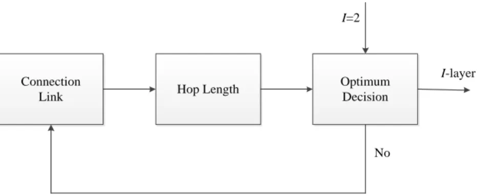
Figure 3 shows a block diagram of the peak-search method. Initially, the parameter I is set as two for the reconfigurable mesh-tree formation. The designated root of the reconfigurable mesh-tree executes the connection link block to calculate the total number of links in the mesh-shaped topology. In the hop length block, the average query hop is defined as the ratio of total number of hops over the number of nodes in the mesh-shaped topology. The query hop is defined as the hop length from each M/S node to the designated node. Finally, the link performance is calculated and compared with its previous I layer in the optimum decision block. This algorithm is iterated until the optimum number of layers I is determined.

Connection

Link Hop Length

Optimum Decision I=2

I-layer

No

Figure 3. Block diagram of the peak-search method. I, the optimum number of layer.

Figure 2.Average path length in a scatternet.

To determine the optimal k layer with the lowest hop length for various topologies, it is essential for a root node to collect all scatternet topology information of various k layers. For the 100-node topology example, a root node forms a mesh-tree scatternet with k = 2, k = 3, k = 4, and up to k = 5 cases. The root node then computes the average hop length of these four cases and determines that k = 4 is the optimal layer with the shortest hop length. However, the optimal layer k is an NP (nondeterministic polynomial) complete problem, since the root node can only acquire the formation topology of its own k layer case instead of all other cases. As a result, the design goal of a reconfigurable mesh-tree algorithm

Energies 2016, 9, 338 7 of 18

attempts to determine the optimum layer k in terms of the mesh-subnet size with lower communication and computation overheads. In addition, the reconfigurable mesh-tree can dynamically compute the optimum layer k when the size of the network changes in the topology maintenance phase.

4. Reconfiguration Formation Algorithm

After scatternet formation, the root node acquires the k-1 layer topology information instead of the complete topology of all layers. To realize and decide the optimum layer k with partial scatternet topology knowledge in the root node, a heuristic algorithm called the peak-search method is proposed in order to achieve the lowest hop length performance of the reconfigurable mesh-tree topology. 4.1. Peak-Search Method

Figure3shows a block diagram of the peak-search method. Initially, the parameter I is set as two for the reconfigurable mesh-tree formation. The designated root of the reconfigurable mesh-tree executes the connection link block to calculate the total number of links in the mesh-shaped topology. In the hop length block, the average query hop is defined as the ratio of total number of hops over the number of nodes in the mesh-shaped topology. The query hop is defined as the hop length from each M/S node to the designated node. Finally, the link performance is calculated and compared with its previous I layer in the optimum decision block. This algorithm is iterated until the optimum number of layers I is determined.

formation topology of its own k layer case instead of all other cases. As a result, the design goal of a

reconfigurable mesh-tree algorithm attempts to determine the optimum layer k in terms of the

mesh-subnet size with lower communication and computation overheads. In addition, the

reconfigurable mesh-tree can dynamically compute the optimum layer k when the size of the

network changes in the topology maintenance phase.

Figure 2. Average path length in a scatternet.

4. Reconfiguration Formation Algorithm

After scatternet formation, the root node acquires the k-1 layer topology information instead of

the complete topology of all layers. To realize and decide the optimum layer k with partial scatternet

topology knowledge in the root node, a heuristic algorithm called the peak-search method is

proposed in order to achieve the lowest hop length performance of the reconfigurable mesh-tree

topology.

4.1. Peak-Search Method

Figure 3 shows a block diagram of the peak-search method. Initially, the parameter I is set as

two for the reconfigurable mesh-tree formation. The designated root of the reconfigurable

mesh-tree executes the connection link block to calculate the total number of links in the

mesh-shaped topology. In the hop length block, the average query hop is defined as the ratio of

total number of hops over the number of nodes in the mesh-shaped topology. The query hop is

defined as the hop length from each M/S node to the designated node. Finally, the link performance

is calculated and compared with its previous I layer in the optimum decision block. This algorithm

is iterated until the optimum number of layers I is determined.

Connection

Link Hop Length

Optimum Decision I=2

I-layer

No

Figure 3. Block diagram of the peak-search method. I, the optimum number of layer.

To realize the peak-search method, a topology configuration algorithm is implemented in the root node of the reconfigurable mesh-tree. During the tree-shaped topology formation phase, a new parameter c is designed as the counter of the hop length from each downstream master to the designated root. With k = I = 2 and c = 0, the root node initially propagates these two parameters in the downstream direction. The new masters (M/S nodes) then increase c by one and decrease k by one until k = 0 in the downstream direction.

During the return connection phase, a new parameter r is also added to represent the number of return links of each M/S node. When each return master connects with additional M/S nodes, the parameter r can be increased by one. Finally, each return master passes its node ID, c and r to the designated root when each master finishes the return connection phase. The root node thus collects sufficient information to calculate the average query path length, the total number of nodes and the total number of return links for the optimum peak-search method decision.

When the optimum I is not located, the root node continuously propagates these two parameters with k = I + 1 and c = 0 in the downstream direction to increase the tree-shaped subnet by one more layer as well as to generate new masters. During the return connection, only the new masters can connect with their neighboring M/S nodes and increase the return link parameter r. This procedure is repeated until the optimum I is determined. When the M/S node cannot connect with its downstream master, it resets parameter r = 0 and sends its ID to the root node to cancel the return connection.

Energies 2016, 9, 338 8 of 18

From this point on, each root node, either in the mesh-subnet or in the tree-subnet, distributively executes the peak-search method to determine the optimum I layer when the sizes of subnets grow. If the complete network topology is acquired at the root node during the maintenance phase, the shortest path of the (I ´ 1), I, and (I + 1) layer can be computed, and the optimal layer can be determined. 4.1.1. Connection Link Block

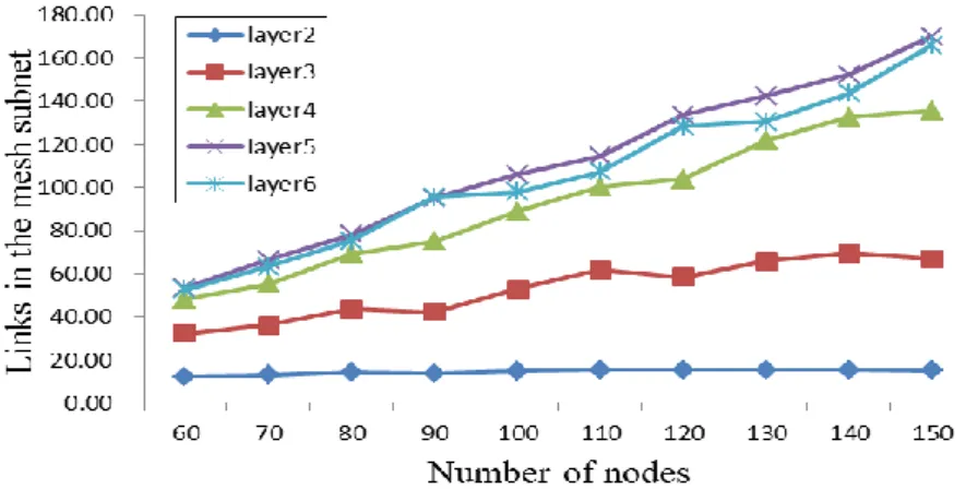
In this block, the designated root calculates the total number of links in the mesh-shaped topology after receiving the node ID and r from each M/S node. The total number of links implies the aggregate throughput performance in the mesh-shaped topology. The total number of links L is then computed as follows: L “ m ÿ i“1 pri`tiq (1)

where m is the number of nodes in the mesh-shaped subnet, riis the number of return links and tiis

the number of tree links for each node m. Figure4shows the total number of links in the mesh-shaped topology for various network sizes. The total number of links in the mesh-shaped subnet increase as the number of layers k increases, except for the k = 6 case, since it is more difficult for this case to satisfy the return condition, as compared with the other cases.

To realize the peak-search method, a topology configuration algorithm is implemented in the root node of the reconfigurable mesh-tree. During the tree-shaped topology formation phase, a new parameter c is designed as the counter of the hop length from each downstream master to the designated root. With k = I = 2 and c = 0, the root node initially propagates these two parameters in the downstream direction. The new masters (M/S nodes) then increase c by one and decrease k by one until k = 0 in the downstream direction.

During the return connection phase, a new parameter r is also added to represent the number of return links of each M/S node. When each return master connects with additional M/S nodes, the parameter r can be increased by one. Finally, each return master passes its node ID, c and r to the designated root when each master finishes the return connection phase. The root node thus collects sufficient information to calculate the average query path length, the total number of nodes and the total number of return links for the optimum peak-search method decision.

When the optimum I is not located, the root node continuously propagates these two parameters with k = I + 1 and c = 0 in the downstream direction to increase the tree-shaped subnet by one more layer as well as to generate new masters. During the return connection, only the new masters can connect with their neighboring M/S nodes and increase the return link parameter r. This procedure is repeated until the optimum I is determined. When the M/S node cannot connect with its downstream master, it resets parameter r = 0 and sends its ID to the root node to cancel the return connection.

From this point on, each root node, either in the mesh-subnet or in the tree-subnet, distributively executes the peak-search method to determine the optimum I layer when the sizes of subnets grow. If the complete network topology is acquired at the root node during the maintenance phase, the shortest path of the (I − 1), I, and (I + 1) layer can be computed, and the optimal layer can be determined.

4.1.1. Connection Link Block

In this block, the designated root calculates the total number of links in the mesh-shaped topology after receiving the node ID and r from each M/S node. The total number of links implies the aggregate throughput performance in the mesh-shaped topology. The total number of links L is then computed as follows:







t

r

L

)

(

where m is the number of nodes in the mesh-shaped subnet,

r

t

Figure 4. The total number of links in the mesh-shaped topology. Figure 4.The total number of links in the mesh-shaped topology. 4.1.2. Hop Length Block Link

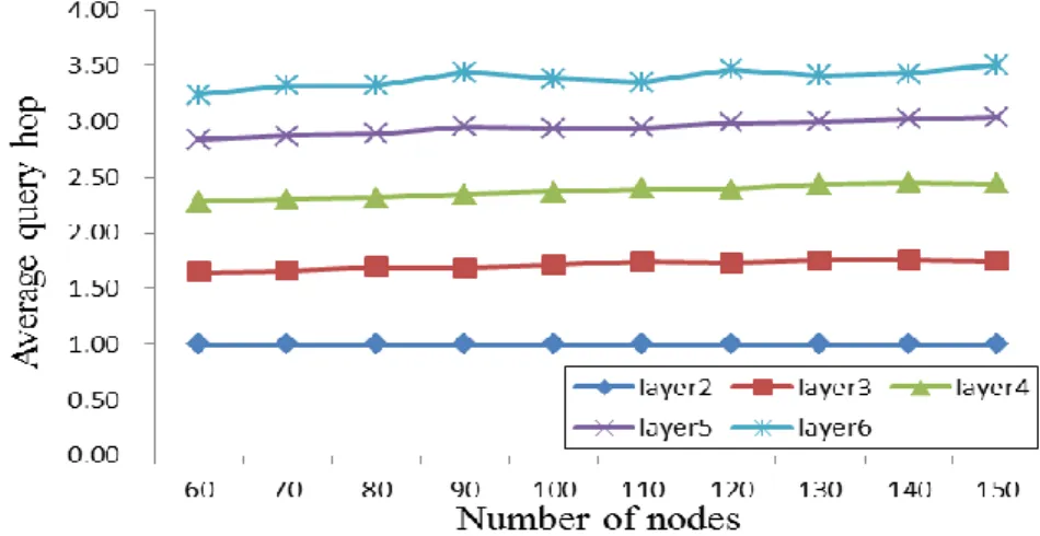
In the hop length block, the average query hop is defined as the ratio of the total number of query hops over the total number of nodes in the mesh-shaped subnet. The average query hop H is computed as follows: H “ p m ÿ i“1 ciq{m (2)

where m is the number of nodes in the mesh-shaped subnet, and ciis the query hop of each node m.

This parameter can be regarded as the maintenance cost in the mesh-shaped topology. The average query hop length increases as the k layer increases, as shown in Figure5.

Energies 2016, 9, 338 9 of 18

4.1.2. Hop Length Block Link

In the hop length block, the average query hop is defined as the ratio of the total number of query hops over the total number of nodes in the mesh-shaped subnet. The average query hop H is computed as follows:

m

m

i

i

c

H

)

/

1

(







where m is the number of nodes in the mesh-shaped subnet, and

c

m. This parameter can be regarded as the maintenance cost in the mesh-shaped topology. The

average query hop length increases as the k layer increases, as shown in Figure 5.

Figure 5. Average query hop in the mesh-shaped topology. 4.1.3. Optimum Decision Block

In this block, link performance PI is defined as the total links LI in the connection link block

over the average query hop HI in the hop length block for various I layers.

PI = LI/HI (3)

Figure 6 shows the sampled average link performance of various layers for different sizes of network. There exists a maximum point as the number of layers either at Layers 3 or 4 for the smaller size of network and at Layers 4 or 5 for the larger size of network. To locate the maximum point, a peak-search method is designed in the optimum decision block.

Initially, I is set as two and the PI is calculated. Then the I = I + 1 for the connection link block

and PI+1 are computed in the optimum decision block. When PI+1 > PI, the optimum decision block

increases I by one and triggers the connection link block again. The link performance ratio of Layer

I + 1 is computed until PI+1 < PI and the decision is made. As a result, I is regarded as the optimum

number of layers, and the algorithm is stopped.

Figure 5.Average query hop in the mesh-shaped topology.

4.1.3. Optimum Decision Block

In this block, link performance PIis defined as the total links LIin the connection link block over

the average query hop HIin the hop length block for various I layers.

PI = LI{HI (3)

Figure6shows the sampled average link performance of various layers for different sizes of network. There exists a maximum point as the number of layers either at Layers 3 or 4 for the smaller size of network and at Layers 4 or 5 for the larger size of network. To locate the maximum point, a peak-search method is designed in the optimum decision block.

Energies 2016, 9, 338 10 of 18

Figure 6. The link performance ratio of peak-search examples.

5. Disjoint Hierarchical Routing

In the reconfigurable mesh-tree network, the designated root can be regarded as the sink node,

and all other nodes are sensors. During packet transmission, the sensor data will forward from each

sensor to the sink node. Therefore, the main traffic congestion is located at the mesh subnet, since

most of the traffic load will pass through this area to its destinations. From the energy consumption

point of view, the nodes nearer the sink forward most of the packets and deplete their batteries more

rapidly than other nodes and become energy holes or hot spot nodes in the network. To balance the

traffic load and address the energy hole problem in the mesh-subnet, two equal disjoint paths are

designed for each node forwarding packets to the sink. In the routing algorithm, each node

generates two equal and disjoint paths to forward sensor data to the sink in the mesh subnet. The

design goal of the routing algorithm is to balance the energy consumption for the hot-spot nodes

and to deliver the packets from one subnet to all the other subnets effectively. Furthermore, each

node with energy harvesting technology acquires additional energy from solar power, which

eliminates the major battery capacity constraint.

In the scatternet formation period, some routing information can be exchanged among masters.

In the first phase of scatternet formation, each master in the mesh-subnet or the tree-subnet keeps a

record of its directly connected master. As a result, a one-hop neighboring path can be easily

formed by connecting all the masters.

In the second phase of scatternet formation, each returning master in the mesh-subnet will

exchange its own piconet information together with a list of its directly connected masters to its

neighboring masters. At the same time, each returning master, including the root, will pass its own

piconet information to its directly connected masters. Here, the directly connected neighboring

piconets within their neighboring k hops of a master are defined as the k-tier piconets of the master.

The associated k-tier piconet information will be stored in the master’s k-tier piconet table. In addition,

those masters affected by the return connection mechanism will update their k-tier piconet tables via

relays. As a result, each master will keep its own piconet information and its k-tier piconet

information. This information is used locally when a node requests a master for a path to deliver

packets.

After completing the second phase of scatternet formation, each master in the mesh-subnet will

have the routing information of all master nodes and store it in a piconet list table. This table

contains a list of all masters. Meanwhile, each master uses the all-pairs Dijkstra’s shortest algorithm

to compute two disjoint shortest paths for any two-piconet pair. This disjoint shortest paths

information is stored in a scatternet routing table, and is used when any slave node asks its master

for routing information to deliver packets and alleviate load balance.

In the tree-subnet of the new root, a routing table is formed by each master node in the

following way: When a leaf node perceives that it is at the end of the tree, it reverts back and

informs its upstream master about itself. Likewise, every informed master then forwards its

descendant information to its upstream master via the tree path established in the first phase, until

Figure 6.The link performance ratio of peak-search examples.

Initially, I is set as two and the PIis calculated. Then the I = I + 1 for the connection link block

and PI+1are computed in the optimum decision block. When PI+1> PI, the optimum decision block

increases I by one and triggers the connection link block again. The link performance ratio of Layer I + 1 is computed until PI+1< PIand the decision is made. As a result, I is regarded as the optimum

number of layers, and the algorithm is stopped. 5. Disjoint Hierarchical Routing

In the reconfigurable mesh-tree network, the designated root can be regarded as the sink node, and all other nodes are sensors. During packet transmission, the sensor data will forward from each

sensor to the sink node. Therefore, the main traffic congestion is located at the mesh subnet, since most of the traffic load will pass through this area to its destinations. From the energy consumption point of view, the nodes nearer the sink forward most of the packets and deplete their batteries more rapidly than other nodes and become energy holes or hot spot nodes in the network. To balance the traffic load and address the energy hole problem in the mesh-subnet, two equal disjoint paths are designed for each node forwarding packets to the sink. In the routing algorithm, each node generates two equal and disjoint paths to forward sensor data to the sink in the mesh subnet. The design goal of the routing algorithm is to balance the energy consumption for the hot-spot nodes and to deliver the packets from one subnet to all the other subnets effectively. Furthermore, each node with energy harvesting technology acquires additional energy from solar power, which eliminates the major battery capacity constraint.

In the scatternet formation period, some routing information can be exchanged among masters. In the first phase of scatternet formation, each master in the mesh-subnet or the tree-subnet keeps a record of its directly connected master. As a result, a one-hop neighboring path can be easily formed by connecting all the masters.

In the second phase of scatternet formation, each returning master in the mesh-subnet will exchange its own piconet information together with a list of its directly connected masters to its neighboring masters. At the same time, each returning master, including the root, will pass its own piconet information to its directly connected masters. Here, the directly connected neighboring piconets within their neighboring k hops of a master are defined as the k-tier piconets of the master. The associated k-tier piconet information will be stored in the master’s k-tier piconet table. In addition, those masters affected by the return connection mechanism will update their k-tier piconet tables via relays. As a result, each master will keep its own piconet information and its k-tier piconet information. This information is used locally when a node requests a master for a path to deliver packets.

After completing the second phase of scatternet formation, each master in the mesh-subnet will have the routing information of all master nodes and store it in a piconet list table. This table contains a list of all masters. Meanwhile, each master uses the all-pairs Dijkstra’s shortest algorithm to compute two disjoint shortest paths for any two-piconet pair. This disjoint shortest paths information is stored in a scatternet routing table, and is used when any slave node asks its master for routing information to deliver packets and alleviate load balance.

In the tree-subnet of the new root, a routing table is formed by each master node in the following way: When a leaf node perceives that it is at the end of the tree, it reverts back and informs its upstream master about itself. Likewise, every informed master then forwards its descendant information to its upstream master via the tree path established in the first phase, until the new root is reached. In this way, every master has its descendant routing information, and the new root node collects all node information. Finally, a simple table-driven routing protocol is used to forward packets on the tree-subnet.

Based on the routing information collected by all the masters in the mesh-subnet and the new roots in the tree-subnet, a disjoint hierarchical routing protocol is developed. This is a proactive routing protocol, and operates in two types of packet transmissions. For the packet transmission of inter-subnets, two shortest routing paths of mesh-subnet are generated to deliver the packets from one subnet to the sink node. In the tree-subnet, the packets are delivered with an optimal path from source to destination in its own subnet by its own root.

In the mesh-routing algorithm, two equal disjoint paths with rechargeable modules are used to improve the network operation time. During packet transmission, each master node periodically exchanges its energy arrival rate and battery capacity with harvested solar energy. Two battery capacity counters, c1 and c2, are defined for each master node, specifying the energy cost from two disjoint routing paths to all destinations.

Several applications can be operated using this mesh-tree network, such as ad hoc or sensor networks. If the destination node is located at the mesh-subnet for sensor network application,

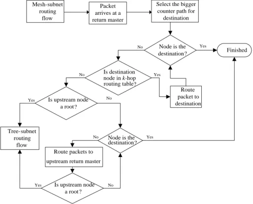
the master will select the path to the destination with the larger counter value, either c1 or c2, and deliver packets to the destination as the sink directly. However, if the destination node is located at another tree-subnet for ad hoc network application, each new root will first pass the packets to its directly-connected master with the largest counter value in the mesh-subnet. This master then examines the destination ID, checks the k-hop routing table of the destination, and passes the packet to the next master, since each master has the k-tier routing information. With the routing assistance of masters in the mesh-subnet, the packets from a source node will be delivered to the correct destination root of the tree-subnet. Finally, the new root passes the sensor packets to its downstream nodes to their final destination. The procedures described above can achieve the packet transmission over inter-subnet communication. The detailed operation diagram of two disjoint paths routing is shown in Figure7.

Energies 2016, 9, 338 12 of 18

Select the bigger counter path for

destination Node is the destination? Finished Is destination node in k-hop routing table? Route packet to destination Node is the destination? Route packets to

upstream return master

Is upstream node a root? Tree-subnet routing flow No Yes Yes Is upstream node a root? No Yes No Yes No No Yes Mesh-subnet routing flow Packet arrives at a return master

Figure 7. Flow diagram of two disjoint paths routing in a mesh-subnet.

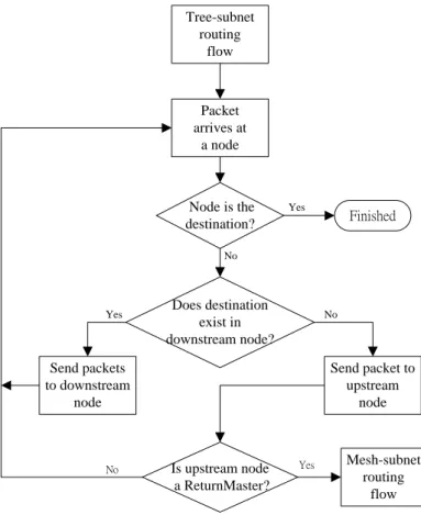
Tree-subnet routing flow Packet arrives at a node Node is the destination? Does destination exist in downstream node? Send packets to downstream node Send packet to upstream node Finished No No Yes Yes Is upstream node a ReturnMaster? No Mesh-subnet routing flow Yes

Figure 8. Tree-subnet routing flow diagram.

6. Scatternet Performance

In this section, the performance of scatternet formation and the routing algorithm are simulated to demonstrate the performance of optimum mesh-tree topography, and compared to BlueHRT. The ring-shaped topology of BlueHRT contains only three nodes in the ring structure, and the tree-shaped topology is extended by all the other nodes. A simulation program is written to evaluate the system performance, including the scatternet, routing and energy efficiency.

Figure 7.Flow diagram of two disjoint paths routing in a mesh-subnet.

For WSN application, a source node with ID = 1 transmits packets to the sink with ID = 10. The source node owns two equal paths, including 1-2-3-4-10 and 1-6-7-8-10, to reach the sink and all forwarding nodes of the two paths are independent. When the event is triggered and the packet is generated from ID = 1, the source node selects the path to the destination with the larger counter value, either c1 or c2, and delivers packets to the destination as the sink directly.

Within a tree-subnet, the routing algorithm for packet transmission is as follows: When any node starts to transmit packets or receive routing packets, it examines its routing information first. If a destination is contained in its routing table, a packet is delivered to the corresponding downstream node. Otherwise, this packet is forwarded to its upstream master. Since the new root possesses the complete spanning tree-subnet routing information, a packet will eventually reach the destination node or pass to the mesh-subnet. The detailed operation diagram of tree-subnet routing is shown in Figure8.

Energies 2016, 9, 338 12 of 18

Select the bigger counter path for

destination Node is the destination? Finished Is destination node in k-hop routing table? Route packet to destination Node is the destination? Route packets to

upstream return master

Is upstream node a root? Tree-subnet routing flow No Yes Yes Is upstream node a root? No Yes No Yes No No Yes Mesh-subnet routing flow Packet arrives at a return master

Figure 7. Flow diagram of two disjoint paths routing in a mesh-subnet.

Tree-subnet routing flow Packet arrives at a node Node is the destination? Does destination exist in downstream node? Send packets to downstream node Send packet to upstream node Finished No No Yes Yes Is upstream node a ReturnMaster? No Mesh-subnet routing flow Yes

Figure 8. Tree-subnet routing flow diagram.

6. Scatternet Performance

In this section, the performance of scatternet formation and the routing algorithm are

simulated to demonstrate the performance of optimum mesh-tree topography, and compared to

BlueHRT. The ring-shaped topology of BlueHRT contains only three nodes in the ring structure,

and the tree-shaped topology is extended by all the other nodes. A simulation program is written to

evaluate the system performance, including the scatternet, routing and energy efficiency.

Figure 8.Tree-subnet routing flow diagram.

6. Scatternet Performance

In this section, the performance of scatternet formation and the routing algorithm are simulated to demonstrate the performance of optimum mesh-tree topography, and compared to BlueHRT. The ring-shaped topology of BlueHRT contains only three nodes in the ring structure, and the tree-shaped topology is extended by all the other nodes. A simulation program is written to evaluate the system performance, including the scatternet, routing and energy efficiency.

6.1. Scatternet Performance

In the scatternet performance simulation, it was assumed that Bluetooth nodes were randomly located within a rectangular area of 40 ˆ 40 m2, while a radio transmission range of 10 m was assumed. The number of simulated nodes ranged from 60 to 150. A set of performance metrics was calculated by averaging over 30 randomly generated topologies for each simulated node number. The simulated mesh-tree topology can be applied to non-uniform distribution applications, such as dense–sparse areas. In addition, the simulation results are shown as follows.

An average hop length between any two nodes was also calculated for these networks. A larger average hop length implies that it would require a longer time to deliver a packet. As shown in Figure9, the optimum mesh-tree method achieved significant performance improvements in terms of the average hop length, as compared to that of BlueHRT. More return links could be connected among the M/S nodes as the number of layers increased; thus, the average path length among nodes could be reduced. In addition, the optimum layer of the peak-search method achieved approximate performance in average hop length, compared with the ideal layer as the optimal topology. However, this peak-search method required the partial 72% topology to locate the optimum layer instead of four full topologies including two, three, four and five layers, in contrast to the ideal layer. From the

Energies 2016, 9, 338 13 of 18

observation of simulation results, most of the optimum decision layer I is either the case of layer = 4 or layer = 5, since both cases almost achieve the lowest hop length for various numbers of nodes.

Energies 2016, 9, 338 13 of 18

6.1. Scatternet Performance

In the scatternet performance simulation, it was assumed that Bluetooth nodes were randomly

located within a rectangular area of 40 × 40 m

, while a radio transmission range of 10 m was

assumed. The number of simulated nodes ranged from 60 to 150. A set of performance metrics was

calculated by averaging over 30 randomly generated topologies for each simulated node number.

The simulated mesh-tree topology can be applied to non-uniform distribution applications, such as

dense–sparse areas. In addition, the simulation results are shown as follows.

An average hop length between any two nodes was also calculated for these networks. A larger

average hop length implies that it would require a longer time to deliver a packet. As shown in Figure 9,

the optimum mesh-tree method achieved significant performance improvements in terms of the

average hop length, as compared to that of BlueHRT. More return links could be connected among

the M/S nodes as the number of layers increased; thus, the average path length among nodes could

be reduced. In addition, the optimum layer of the peak-search method achieved approximate

performance in average hop length, compared with the ideal layer as the optimal topology.

However, this peak-search method required the partial 72% topology to locate the optimum layer

instead of four full topologies including two, three, four and five layers, in contrast to the ideal

layer. From the observation of simulation results, most of the optimum decision layer I is either the

case of layer = 4 or layer = 5, since both cases almost achieve the lowest hop length for various

numbers of nodes.

Figure 9. Average path length in a scatternet.

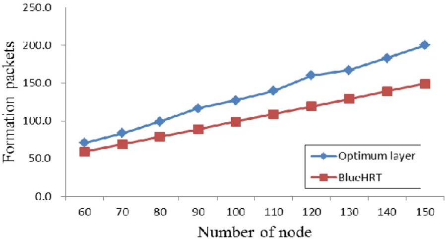
As shown in Figure 10, the reconfigurable mesh-tree required more formation packets in terms

of energy cost than BlueHRT did. The formation packets are counted as the total number of

communication packets in the mesh-subnet and the formation packets of all the other tree subnets.

However, this formation packet overhead was only generated during the scatternet formation

phase.

Figure 10. Average number of formation packets.

Figure 9.Average path length in a scatternet.

As shown in Figure 10, the reconfigurable mesh-tree required more formation packets in terms of energy cost than BlueHRT did. The formation packets are counted as the total number of communication packets in the mesh-subnet and the formation packets of all the other tree subnets. However, this formation packet overhead was only generated during the scatternet formation phase.

6.1. Scatternet Performance

In the scatternet performance simulation, it was assumed that Bluetooth nodes were randomly

located within a rectangular area of 40 × 40 m

, while a radio transmission range of 10 m was

assumed. The number of simulated nodes ranged from 60 to 150. A set of performance metrics was

calculated by averaging over 30 randomly generated topologies for each simulated node number.

The simulated mesh-tree topology can be applied to non-uniform distribution applications, such as

dense–sparse areas. In addition, the simulation results are shown as follows.

An average hop length between any two nodes was also calculated for these networks. A larger

average hop length implies that it would require a longer time to deliver a packet. As shown in Figure 9,

the optimum mesh-tree method achieved significant performance improvements in terms of the

average hop length, as compared to that of BlueHRT. More return links could be connected among

the M/S nodes as the number of layers increased; thus, the average path length among nodes could

be reduced. In addition, the optimum layer of the peak-search method achieved approximate

performance in average hop length, compared with the ideal layer as the optimal topology.

However, this peak-search method required the partial 72% topology to locate the optimum layer

instead of four full topologies including two, three, four and five layers, in contrast to the ideal

layer. From the observation of simulation results, most of the optimum decision layer I is either the

case of layer = 4 or layer = 5, since both cases almost achieve the lowest hop length for various

numbers of nodes.

Figure 9. Average path length in a scatternet.

As shown in Figure 10, the reconfigurable mesh-tree required more formation packets in terms

of energy cost than BlueHRT did. The formation packets are counted as the total number of

communication packets in the mesh-subnet and the formation packets of all the other tree subnets.

However, this formation packet overhead was only generated during the scatternet formation

phase.

Figure 10. Average number of formation packets.

6.2. Routing Performance

In the simulation scenario, the scatternet topologies were constructed using the scatternet formation algorithms described in Section3. Overall, 10 topologies were simulated, each with 60 nodes randomly distributed in the same geographical area. The optimum layer k is determined as three by the peak-search method for the 60-node samples. Table1summarizes the simulation parameters.

The average packet throughput is defined as the ratio of the total number of successfully completed routing packets over the total simulation time in seconds. This parameter reflects the transmission capacity of a scatternet.

The simulation results for the average packet throughput comparison between the reconfigurable mesh-tree and BlueHRT are presented in Figure11. In BlueHRT, the throughput initially increases as the packet generation rate increases. However, this throughput slowly increases as the packet generation rate increases beyond three packets/node/s. This is because in a ring with tree-shaped

Energies 2016, 9, 338 14 of 18

architecture, packets tend to be queued at the nodes of the ring-subnet, and scatternet congestion is more likely to occur earlier.

Table 1.The simulation parameters.

Simulation Time (s) 20

Number of nodes 60

Optimum layer for 60-node samples 3

N-tier in all masters 4

Traffic pattern Poisson arrival

Scheduling scheme Round robin

Routing protocols Hierarchical Routing

Packet transmission Source routing

FIFO buffer size 400 Packets

Source-destination pair Randomly selected

Query or reply packet 1 Time slot

Data packet (for each routing session) 5 Time slots

Each routing session 1 Data packet

FIFO, first input first output.

6.2 Routing Performance

In the simulation scenario, the scatternet topologies were constructed using the scatternet

formation algorithms described in Section 3. Overall, 10 topologies were simulated, each with 60

nodes randomly distributed in the same geographical area. The optimum layer k is determined as

three by the peak-search method for the 60-node samples. Table 1 summarizes the simulation

parameters.

Table 1. The simulation parameters.

Simulation Time (s) 20

Number of nodes 60

Optimum layer for 60-node samples 3

N-tier in all masters 4

Traffic pattern Poisson arrival Scheduling scheme Round robin

Routing protocols Hierarchical Routing Packet transmission Source routing

FIFO buffer size 400 Packets Source-destination pair Randomly selected

Query or reply packet 1 Time slot Data packet (for each routing session) 5 Time slots

Each routing session 1 Data packet FIFO, first input first output.

The average packet throughput is defined as the ratio of the total number of successfully

completed routing packets over the total simulation time in seconds. This parameter reflects the

transmission capacity of a scatternet.

The simulation results for the average packet throughput comparison between the

reconfigurable mesh-tree and BlueHRT are presented in Figure 11. In BlueHRT, the throughput

initially increases as the packet generation rate increases. However, this throughput slowly

increases as the packet generation rate increases beyond three packets/node/s. This is because in a

ring with tree-shaped architecture, packets tend to be queued at the nodes of the ring-subnet, and

scatternet congestion is more likely to occur earlier.

0 50 100 150 200 250 300 350 1 2 3 4 5 6 7 8 9 10

Packet generation rate (packets/node/sec)

P ac k et t h ro u g h p u t (p ac k et s/ se c) Layer=2 Layer=3 Layer=4 Layer=5 BlueHRT

Figure 11. Average packet throughput of mesh-tree and BlueHRT.

In a mesh-tree topology, the average packet throughput increases continuously as the routing

packet generation rate increases. In general, the mesh-tree has much better throughput performance

than BlueHRT in layer k = 2, 3 and 4 cases. This is because the hierarchical routing method, together

with the mesh-subnet, significantly enhances the system performance. From the observation of the

simulation, the throughput increases as the size of the mesh subnet increases. When the packet

generation rate is greater than six, the k = 3 and 4 cases achieve better throughput performance than

Figure 11.Average packet throughput of mesh-tree and BlueHRT.

In a mesh-tree topology, the average packet throughput increases continuously as the routing packet generation rate increases. In general, the mesh-tree has much better throughput performance than BlueHRT in layer k = 2, 3 and 4 cases. This is because the hierarchical routing method, together with the mesh-subnet, significantly enhances the system performance. From the observation of the simulation, the throughput increases as the size of the mesh subnet increases. When the packet generation rate is greater than six, the k = 3 and 4 cases achieve better throughput performance than the k = 2 case since they generate more return links to increase the size of the mesh-subnet. In addition, the k = 5 case achieves the worst throughput performance as BlueHRT since this case almost achieves the tree structure and is not suitable for the reconfigurable mesh-tree network.

The average packet delay metric is defined as the average packet transmission time from the first transmitted bit at the source node to the last received bit at the destination node for every routing packet. The average packet delay for any two node pair in the scatternet is mainly governed by three factors, which include average path length, average intra-piconet scheduling delay and average inter-piconet switching delay in the scatternet.

Figure12shows the average packet delay performance of the reconfigurable mesh-tree and BlueHRT. In BlueHRT, the delay metric rapidly increases as the packet generation rate increases above two packets/nodes, and saturates when the packet generation rate increases above four packets/nodes.