挖掘可語意解讀之知識並預測蛋白質之殘基與去氧核醣核酸之鍵結

國立交通大學

生物資訊所

碩士論文

挖掘可語意解讀之知識並

預測蛋白質之殘基與去氧核醣核酸之鍵結

Mining Interpretable Knowledge and

Predicting Residues of DNA-Binding Proteins

研 究 生：張嘉芸

指導教授：何信瑩 教授

挖掘可語意解讀之知識並

預測蛋白質之殘基與去氧核醣核酸之鍵結

Mining Interpretable Knowledge and

Predicting Residues of DNA-Binding Proteins

研 究 生：張嘉芸 Student：Chia-Yun Chang

指導教授：何信瑩

Advisor：Shinn-Ying Ho

國立交通大學

生物資訊所

碩士論文

A Thesis Submitted to Institute of Bioinformatics

National Chiao Tung University in partial Fulfillment of the Requirements

for the Degree of Master in Bioinformatics

June 2006

Hsinchu, Taiwan, Republic of China

中華民國九十五年六月

挖掘可語意解讀之知識並預測蛋白質之殘基與去氧核醣核酸之鍵結 學生：張嘉芸 指導教授：何信瑩 國立交通大學生物資訊所碩士班 摘 要 本論文探討哪一個殘基能夠和去氧核醣核酸形成鍵結的預測問題，並且擷取以可 語意解讀鍵結和非鍵結規則來表現的知識。在使用機械學習的方法時，分類器的 選擇將會影響預測的結果及知識取得。在生物資訊領域中常用的分類器在預測上 有著各種不同的應用並且可產生不錯的結果，但是其中的許多方法缺少可語意解 讀的特性。在這篇論文中，使用可語意解讀之分類器，也就是用規則式決策樹系 統來研究和去氧核醣核酸鍵結之蛋白質問題，它有下列幾項優點：能直接處理符 號式的特徵、可得特徵重要度的排名以及能挖掘可讀的知識。 在過去已有許多預測和去氧核醣核酸鍵結之蛋白質的研究，最近使用類神經 網路系統得到 79.1%的正確率 61.1%的淨預測值，在此研究中所使用的決策樹系 統，以同樣的和去氧核醣核酸鍵結之蛋白質資料，並使用相同的特徵，可發現不 論在正確率或是淨預測值皆有改善。當使用本文所提新特徵的情況下，更可讓正 確率達到 79.72%，淨預測值達到 72.90%。因為我們希望挖掘出的規則能更具代 表性，所以我們使用了共 982 筆大量的去氧核醣核酸鍵結之蛋白質資料，來進行 資料挖掘的工作。結果顯示出除了眾所周知的和溶劑接觸的相對面積外，殘基周 圍的電荷分佈和殘基的類別都在預測中扮演重要的角色。同時，這些由決策樹系 統挖掘出的規則顯示，其他的特徵也給予我們在處理和去氧核醣核酸鍵結之蛋白 質的預測問題提供一定的幫助。

Mining Interpretable Knowledge and Predicting Residues of DNA-Binding Proteins

Student：Chia-Yun Chang Advisor：Shinn-Ying Ho Institute of Bioinformatics

National Chiao Tung University

Abstract

In the thesis, both prediction of DNA-binding cites in proteins and knowledge acquisition in terms of interpretable binding and nonbinding rules are investigated. The classifier design using machine learning approaches would affect performances of the prediction and knowledge acquisition. The commonly-used prediction methods have a variety of applications and effective results in prediction problems, but their results suffer from low interpretabilities. Therefore, this thesis proposes an interpretable classifier based on a decision tree method to handle the DNA-binding protein problems. It has several advantages: capability of directly dealing with symbol features, ranking importance of features and mining interpretable knowledge.

In the past, a lot of researches studied the prediction problem in DNA-binding proteins. Recently, the existing neural network method has 79.1% accuracy and 61.1% net prediction (NP=(Sensitivity+Specificity)/2)). The proposed decision tree system can obtain better performance in terms of both accuracy and NP using the same features in these protein-DNA complex dataset. And when using the proposed feature set, the advanced performance has 79.72% accuracy and NP = 72.90%. To obtain more representative rules, we established a large dataset with 982 DNA-binding proteins. From the derived rule base, it reveals that besides well-known relative accessible surface area, the electric charge distribution near the residue and the amino acid groups in the proteins are also significant characteristics in prediction. At the same time, the listed rules mined by the decision tree system explain that other features could assist us in DNA-binding protein prediction.

Acknowledgements

The most appreciation is for my advisor, Dr. Shinn-Ying Ho. Because of his advices and instructions, I could finish this work. I am very grateful for his suggestions on the research. Without his comments on writing the thesis, I can’t accomplish it. Thanks my advisor very much. And I also thank to everyone in Ho’s lab. This is a pleasurable experience of working together. Finally, I would thank my whole family, for their support during past twenty-four years.

Contents

摘 要...i

Abstract...ii

Acknowledgements ... iii

Contents ...iv

List of Tables ...vi

List of Figures...vii

1 Introduction...1

1.1 Motivation...1

1.2 Survey of the Related Works ...2

1.3 Sketch of the Thesis ...3

1.4 Organization...4

2 Materials ...5

2.1 Data sets ...5

2.1.1 The Source of the PDNA-62...5

2.1.2 The Source of the PDNA-982...5

2.1.3 To determine the binding and nonbinding criterion...6

2.2 Feature sets...6

2.2.1 The used feature sets in Ahmad et al. (2004)...10

2.2.2 The proposed feature sets...10

3 Methods...14

3.1 The proposed decision tree method ...14

3.1.1 The Parameters Setting ...16

3.1.3 Training and Test...18

3.2 Accuracy scores ...18

3.3 The process in the experiment ...19

4 Result...22

4.1 Performance evaluation ...22

4.1.1 Using original feature sets in PDNA-62 ...22

4.1.2 Using the proposed feature sets in PDNA-62 ...24

4.2 Knowledge acquisition...26

4.2.1 The importance order of the features ...27

4.2.2 Rules mining ...27

5 Conclusion ...32

5.1 DT for DNA-binding protein prediction...32

5.2 Knowledge acquisition by DT ...33

5.3 Future work ...33

List of Tables

2.1. PDB codes of PDNA-62 ...6

2.2. PDB codes of PDNA-982 ...7

2.3. The relationship between the twenty amino acids and five groups...11

2.4. The amino acid and its pI value...12

4.1. Performance of the different feature sets ...25

4.2. The ranked importance of proposed features ...28

4.3. The nonbinding rules for DNA-binding proteins...29

List of Figures

2.1. The parameter setting in PDB advanced search to obtain the PDNA-982. ..7

2.2. An example for electric charge near the surfaces of the residues ...12

3.1. An example for decision tree method...15

3.2. The basic decision tree algorithm ...15

3.3. Over-fitting in decision tree learning ...16

3.4. An example for getting the features ...20

3.5. Illumination of the framework of the thesis ...21

4.1. To compare NP value and total accuracy in different parameters ...23

4.2. To compare the results between Ahmad et al. (2004) and our proposed method...24

4.3. To compare the results in different parameters...25

Chapter 1

Introduction

1.1 Motivation

The problem about DNA-binding proteins is a significant topic for biochemical discussion because the proteins often relate gene regulation. It is mainly controlled via binding of transcription factors to DNA for promoting or repressing gene expression. These transcription factors are mainly DNA-binding proteins coded by 2~3% of the genome in prokaryotes and 6~7% in eukaryotes [1-3]. The thesis would predict which residues are able to bind with DNA and further mining the binding and nonbinding rules. Many researchers in the field of bioinformatics had proposed all kinds of methods. Recently, a better result had been showed in [4]. This paper had used neuron network (NN) system and input four features consisting of solvent accessibility and surrounding residues. However, the disadvantages of the NN method are twofold: 1) the prediction is not linguistically interpretable and 2) it is difficult to deal with a large number of input features [5, 6].

We deem the research have a choice to be improved. Therefore, we propose decision tree (DT) method [7]. It not only obtains the better prediction performance on the problem, but also lists the interpretable knowledge. Besides the above-mentioned advantage, the capability of direct dealing with symbol features, the rank of the major features and knowledge acquisition, DT method could handle higher dimension problem [5-8]. In addition to the same features with [4], we also establish another feature set with 11 candidate features for encouraging prediction by

additionally inputting the secondary structure and other information of the residues. Finally, we collect a large data, 982 DNA-binding proteins, in order to mine the representative knowledge in DNA-binding proteins. The knowledge about DNA-binding proteins will be displayed in the thesis later.

1.2 Survey of the Related Works

DNA-binding proteins usually affect the regulation and expression of DNA in organisms. X-ray crystallographic and NMR spectroscopic analysis on DNA-binding proteins have provided valuable information about the general features of these complexes. Computer-aided analysis will be a significant factor when the data is continually growing. It is desirable to analyze DNA-binding proteins via accurate prediction of binding sites and understanding of relations between DNA and protein structures.

Recently, various methods have been proposed to identify valuable features of DNA-binding proteins. Ahmad et al. (2005) researched DNA binding sites in proteins according to PSSM-based [9]. Ahmad et al. (2004) analyzed and predicted DNA-binding protein based on composition, sequence and structural information by neural network (NN) method [4]. Shanahan et al. (2004) identified DNA-binding proteins using structural motifs and electrostatic potential [10]. Luscombe and Thornton (2002) investigated protein-DNA interactions based on amino acid conservation and the effects of mutations on binding specificity [11]. Selvaraj et al. (2002) analyzed symmetric/asymmetric and cognate/non-cognate binding by specificity of protein-DNA recognition [12]. Pabo and Nekludova (2000) developed geometrical models for characterizing protein-DNA interfaces [13]. Nadassy et al. (1999) analyzed structural features of protein-nucleic acid recognition sites [14]. Kono and Sarai (1999) presented a structure-based method for prediction of DNA target sites by regulatory proteins[15]. According to [16-18], DNA-binding protein problem is a significant topic, but there are a lot of complicated and waiting for be solved difficulties. Consequently, we want to do research in this field further.

1.3 Sketch of the Thesis

The previous research, [4], had provided a successful recognition and statistic in the residues of these proteins. And then, [9] researched DNA binding sites by using PSSM-based. In the thesis, our goal is to mine the knowledge from DNA-binding protein complexes. Consequently, the used model in this thesis is close to [4].

There are two main topics in this thesis. One is to improve the performance of the prediction. Another is knowledge acquisition from DNA-binding proteins. The two objectives could be achieved by proposing an efficient classifier and more useful feature set. Therefore, the step 1 is to propose a rule-based decision tree (DT) method to classify these data with identical feature sets from [4]. According to the results of this part, the performances of the two machine learning methods - NN and DT, for this research could be compared easily. In our work, we find DT method really suits the problem than NN. And step 2, new features are input DT system. Besides original features, we add secondary structure, the electric charge near the residue and the group information. Although the number of candidate features is increased from 4 to 11, DT system has the capability of dealing with the higher dimension problem. These results about using the new feature sets are further improved. In this part of the research, we derive the appropriate feature set from these outcomes to do the advanced experiment, knowledge acquisition.

Step 3 in our research, a large DNA-binding protein data from PDB is obtained in order to mine more creditable knowledge. From these data, the ranked importance of 11 features will be listed, and the significant features include relative accessible surface area (rASA) [19-21], the electric charge distribution near the residue (EC) and its amino acid group. We could discover which features have decisive influence for the growth of the tree and indirectly affect the performance of the prediction. At the same time, the binding and nonbinding rules will be acquired. That function, mining knowledge, is useful property of DT method. The information could give us the verification from biological view. And these rules might be capable to supply the

detailed material for us to do advance analysis in biology.

1.4 Organization

The monograph is divided into three major parts. The first part (Chapter 2) is devoted to the used data and feature sets. The second part (Chapter 3) is dedicated to decision tree (DT) method and the processes in the experiment. The third part (Chapter 4) concerns to the prediction results and knowledge discovery. And the detail organization is as follows.

Chapter 2 displays two portions. One is which protein data we are gotten from PDB and their obtained reasons. Another is how the used features are derived from above-mentioned data set.

Chapter 3 presents the proposed decision tree (DT) system in earlier part. Besides the introduction, algorithm, evaluation equation, parameter setting and input data-form will be described. And then, the used accuracy scores and the experimental processes will be also showed.

Chapter 4 contains two major subjects. One shows the prediction performance for DNA-binding proteins by using different parameters or feature sets. Another is to respect with knowledge mining from data, inclusive of the ranked importance of these features, the binding and nonbinding rules for these proteins.

Chapter 5 concludes the thesis. It starts with the summary of the goals and the significance of DNA-binding protein predication problem. The proposed machine learning method, its parameter setting and feature set are concluded for the prediction performance and knowledge acquisition. Finally, we will refer to the advanced research in the topic in future work.

Chapter 2

Materials

2.1 Data sets

There are two datasets which we use to evaluate our DT method in the thesis. However, these two datasets devote to the different function. To compare the accuracy of the prediction results fairly, we must consider the sequence identity in proteins. Therefore, the identity in PDNA-62 is limited, its identity < 25%. But in second part, we must expand the number of the dataset, because we would like to mine representative knowledge and hope that could respond to the importance degree of the rules in DNA-binding protein distribution. For these reasons, the protein identity in PDNA-982 is not limited.

2.1.1

The Source of the PDNA-62

PDNA-62 in the research is the same with the previous research [4, 9, 12]. These used data sets of protein-DNA complexes from the Protein Data Bank (PDB) are given in Table 2.1. Identity among the sequences is < 25%, and the resolution of the structures is 2.5 Å or better.

2.1.2

The Source of the PDNA-982

The more creditable binding and nonbinding rules are desired in order to mine the biological meaning further. And the objective in this part is the significance of these rules could be responded to DNA-binding protein distribution. More DNA-binding protein data are collected in the proportion of the thesis and named as PDNA-982.

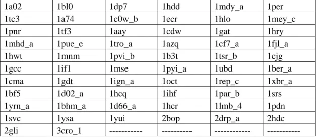
Table 2.1. PDB codes of PDNA-62: These protein–DNA complexes selected for prediction of binding sites

1a02 1bl0 1dp7 1hdd 1mdy_a 1per

1tc3 1a74 1c0w_b 1ecr 1hlo 1mey_c

1pnr 1tf3 1aay 1cdw 1gat 1hry

1mhd_a 1pue_e 1tro_a 1azq 1cf7_a 1fjl_a

1hwt 1mnm 1pvi_b 1b3t 1tsr_b 1cjg

1gcc 1if1 1mse 1pyi_a 1ubd 1ber_a

1cma 1gdt 1ign_a 1oct 1rep_c 1xbr_a

1bf5 1d02_a 1hcq 1ihf 1par_b 1srs

1yrn_a 1bhm_a 1d66_a 1hcr 1lmb_4 1pdn

1svc 1ysa 1yui 2bop 2drp_a 2hdc

2gli 3cro_1 --- --- --- ---

These data are acquired from the processes in PDB database. The advanced search is used and these parameters are set in Figure 2.1 (The website is http://www.rcsb.org/pdb/advSearch.do). These items, “Contains Protein” and “Contains DNA”, in “molecule or chain type” are chosen because we would like to get more data probably. And then, the fragments, the numbers of the residues being less than 10, are taken out from these dataset. Finally, we obtain 982 DNA-binding proteins. PDB codes of PDNA-982 are given in Table 2.2.

2.1.3

To determine the binding and nonbinding criterion

We define the amino acid as a binding residue if its side chain or backbone atoms fell within a cutoff distance of 3.5 Å from any atom within a binding DNA. On the contrary, the data which does not conform to the above definition are nonbinding residues [4, 9, 12]. All binding or nonbinding situations of the residues in the thesis are labeled by this criterion.

2.2 Feature sets

The used features sets in the thesis have two major parts. The application of the feature sets in our proposed method will be expressed in next chapter. In this chapter, we only describe the acquiring method of the feature sets.

Figure 2.1. The parameter setting in PDB advanced search to obtain the PDNA-982: To search for the data, we gave the value of the parameters in PDB database.

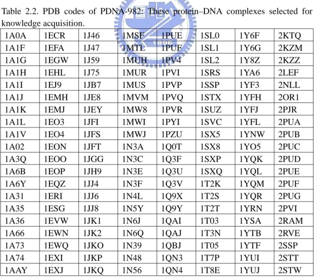
Table 2.2. PDB codes of PDNA-982: These protein–DNA complexes selected for knowledge acquisition.

1A0A 1ECR 1J46 1MSF 1PUE 1SL0 1Y6F 2KTQ

1A1F 1EFA 1J47 1MTL 1PUF 1SL1 1Y6G 2KZM

1A1G 1EGW 1J59 1MUH 1PV4 1SL2 1Y8Z 2KZZ

1A1H 1EHL 1J75 1MUR 1PVI 1SRS 1YA6 2LEF

1A1I 1EJ9 1JB7 1MUS 1PVP 1SSP 1YF3 2NLL

1A1J 1EMH 1JE8 1MVM 1PVQ 1STX 1YFH 2OR1

1A1K 1EMJ 1JEY 1MW8 1PVR 1SUZ 1YFJ 2PJR

1A1L 1EO3 1JFI 1MWI 1PYI 1SVC 1YFL 2PUA

1A1V 1EO4 1JFS 1MWJ 1PZU 1SX5 1YNW 2PUB

1A02 1EON 1JFT 1N3A 1Q0T 1SX8 1YO5 2PUC

1A3Q 1EOO 1JGG 1N3C 1Q3F 1SXP 1YQK 2PUD

1A6B 1EOP 1JH9 1N3E 1Q3U 1SXQ 1YQL 2PUE

1A6Y 1EQZ 1JJ4 1N3F 1Q3V 1T2K 1YQM 2PUF

1A31 1ERI 1JJ6 1N4L 1Q9X 1T2S 1YQR 2PUG

1A35 1ESG 1JJ8 1N5Y 1Q9Y 1T2T 1YRN 2PVI

1A36 1EVW 1JK1 1N6J 1QAI 1T03 1YSA 2RAM

1A66 1EWN 1JK2 1N6Q 1QAJ 1T3N 1YTB 2RVE

1A73 1EWQ 1JKO 1N39 1QBJ 1T05 1YTF 2SSP

1A74 1EXI 1JKP 1N48 1QN3 1T7P 1YUI 2STT

1AHD 1EYG 1JKR 1NFK 1QN5 1T8I 1YZ8 2UP1

1AIS 1EYU 1JMC 1NG9 1QN6 1T9I 1Z1B 3BAM

1AKH 1F0O 1JNM 1NGM 1QN7 1T9J 1Z1C 3BDP

1AM9 1F0V 1JT0 1NH2 1QN8 1T38 1Z1G 3CRO

1AN2 1F2I 1JWL 1NH3 1QN9 1T39 1Z9C 3CRX

1AN4 1F4K 1JX4 1NJW 1QNA 1TAU 1Z19 3GAT

1AOI 1F4R 1JXL 1NJX 1QNB 1TC3 1Z63 3HDD

1APL 1F4S 1K3W 1NJY 1QNC 1TDZ 1ZAA 3HTS

1AU7 1F5E 1K3X 1NJZ 1QNE 1TEZ 1ZAY 3KTQ

1AWC 1F5T 1K4S 1NK0 1QP0 1TF3 1ZBB 3MHT

1AZ0 1F6O 1K4T 1NK2 1QP4 1TF6 1ZET 3ORC

1AZP 1F44 1K6O 1NK3 1QP7 1TGH 1ZG1 3PJR

1AZQ 1F66 1K7A 1NK4 1QP9 1TK0 1ZG5 3PVI

1B01 1FIU 1K8G 1NK5 1QPI 1TK5 1ZGW 4BDP

1B3T 1FJL 1K61 1NK6 1QPS 1TK8 1ZJM 4CRX

1B8I 1FJX 1K78 1NK7 1QPZ 1TKD 1ZJN 4DPV

1B69 1FLO 1K79 1NK8 1QQA 1TL8 1ZME 4GAT

1B72 1FN7 1K82 1NK9 1QQB 1TN9 1ZQA 4KTQ

1B94 1FOK 1KB2 1NKB 1QRH 1TQE 1ZQB 4MHT

1B95 1FOS 1KB4 1NKC 1QRI 1TRO 1ZQC 4RVE

1B96 1FW6 1KB6 1NKE 1QRV 1TRR 1ZQD 4SKN

1B97 1FYK 1KBU 1NKP 1QSL 1TSR 1ZQE 5CRX

1BBX 1FYL 1KC6 1NLW 1QSS 1TTU 1ZQF 5GAT

1BC7 1FYM 1KDH 1NNE 1QSY 1TUP 1ZQG 5MHT

1BC8 1FZP 1KEG 1NNJ 1QTM 1TV9 1ZQH 6CRO

1BDH 1G2D 1KFS 1NOP 1QUM 1TVA 1ZQI 6GAT

1BDI 1G2F 1KFV 1NOY 1QX0 1TW8 1ZQJ 6MHT

1BDT 1G4D 1KIX 1NVP 1QZG 1TX3 1ZQK 6PAX

1BDV 1G9Y 1KLN 1NWQ 1QZH 1U0C 1ZQL 7GAT

1BF4 1G9Z 1KQQ 1NZB 1R0A 1U0D 1ZQM 7ICE

1BF5 1G38 1KRP 1O3Q 1R0N 1U1K 1ZQN 7ICF

1BG1 1GA5 1KSP 1O3R 1R0O 1U1L 1ZQO 7ICG

1BGB 1GAT 1KSX 1O3S 1R2Y 1U1M 1ZQP 7ICH

1BHM 1GAU 1KSY 1O3T 1R2Z 1U1N 1ZQQ 7ICI

1BJ6 1GCC 1KU7 1O4X 1R4I 1U1O 1ZQR 7ICJ

1BL0 1GD2 1KX3 1OCT 1R4O 1U1P 1ZQS 7ICK

1BNK 1GDT 1KX4 1ODG 1R4R 1U1Q 1ZQT 7ICL

1BNZ 1GJI 1KX5 1ODH 1R7M 1U1R 1ZR2 7ICM

1BP7 1GLU 1L1M 1OE4 1R8D 1U1Y 1ZR4 7ICN

1BPX 1GM5 1L1T 1OE5 1R8E 1U3E 1ZS4 7ICO

1BPY 1GT0 1L1Z 1OE6 1R49 1U4B 1ZTT 7ICP

1BRN 1GU4 1L2C 1OH6 1RAM 1U8R 1ZX4 7ICR

1BSS 1GU5 1L2D 1OH7 1RB8 1U35 1ZYQ 7ICS

1BSU 1GXP 1L3L 1OH8 1RBJ 1U45 1ZZI 7ICT

1BUA 1H0M 1L3S 1OJ8 1RC8 1U47 1ZZJ 7ICU

1BVO 1H6F 1L3T 1OMH 1RCN 1U48 2A0I 7ICV

1BY4 1H8A 1L3U 1ORN 1RCS 1U49 2A6O 7MHT

1C0W 1H9D 1L3V 1ORP 1REP 1U78 2A66 8ICA

1C7U 1H9T 1L5U 1OSB 1RFF 1UA0 2ACJ 8ICB

1C7Y 1H88 1LAT 1OSL 1RFI 1UA1 2AGO 8ICC

1C8C 1H89 1LAU 1OTC 1RG1 1UAA 2AGP 8ICE

1C9B 1HAO 1LB2 1OUP 1RG2 1UBD 2AGQ 8ICF

1CA5 1HAP 1LCC 1OUQ 1RGT 1UUT 2ALZ 8ICG

1CA6 1HBX 1LCD 1OUZ 1RGU 1V14 2AOQ 8ICH

1CBV 1HCQ 1LE5 1OWF 1RH0 1V15 2AOR 8ICI

1CDW 1HCR 1LE8 1OWG 1RH6 1VAS 2AQ4 8ICJ

1CEZ 1HDD 1LE9 1OWR 1RIO 1VFC 2AXY 8ICK

1CF7 1HF0 1LEI 1OZJ 1RM1 1VKX 2B0D 8ICL

1CGP 1HHT 1LFU 1P3A 1RNB 1VOL 2B0E 8ICM

1CIT 1HI0 1LLI 1P3B 1RPE 1VPW 2BAM 8ICN

1CJG 1HJB 1LLM 1P3F 1RPZ 1VRL 2BDP 8ICO

1CKQ 1HJC 1LMB 1P3G 1RR8 1VRR 2BGW 8ICP

1CKT 1HLO 1LO1 1P3I 1RRC 1W0T 2BJC 8ICQ

1CL8 1HLV 1LPQ 1P3K 1RRJ 1W0U 2BOP 8ICR

1CLQ 1HLZ 1LQ1 1P3L 1RRQ 1W7A 2BPA 8ICS

1CMA 1HRY 1LRR 1P3M 1RRS 1W36 2BPF 8ICT

1CO0 1HRZ 1LV5 1P3O 1RTA 1WD0 2BPG 8ICU

1CQT 1HU0 1LWS 1P3P 1RTD 1WD1 2BQ3 8ICV

1CRX 1HUO 1LWT 1P4E 1RUN 1WET 2BQR 8ICW

1CW0 1HUT 1LWV 1P5W 1RUO 1WTB 2BQU 8ICX

1CYQ 1HUZ 1LWW 1P7D 1RV2 1WTE 2BR0 8ICY

1CZ0 1HVN 1LWY 1P7H 1RV5 1WTO 2BZF 8ICZ

1D0E 1HVO 1M0E 1P8K 1RVA 1WTP 2C0B 8MHT

1D1U 1HW2 1M1A 1P34 1RVB 1WTQ 2C2D 9ANT

1D02 1HWT 1M3H 1P47 1RVC 1WTR 2C2E 9ICA

1D2I 1I3J 1M3Q 1P51 1RXV 1WTV 2C2R 9ICB

1D3U 1I6J 1M5R 1P59 1RXW 1WTW 2C5.0R 9ICC

1D5Y 1I7D 1M5X 1P71 1RYR 1WTX 2C7O 9ICE

1D8Y 1I8M 1M06 1P78 1RYS 1WVL 2C7P 9ICF

1D66 1IAW 1M6X 1PA6 1RZ9 1X0F 2C7Q 9ICG

1DC1 1IC8 1M07 1PAR 1RZR 1X9M 2C7R 9ICH

1DCT 1ID3 1M18 1PDN 1RZT 1X9N 2C22 9ICI

1DE8 1IG4 1MA7 1PGZ 1S0N 1X9W 2CGP 9ICK

1DE9 1IG7 1MDM 1PH1 1S0O 1XBR 2CRX 9ICL

1DEW 1IG9 1MDY 1PH2 1S6M 1XC8 2CV5 9ICM

1DFM 1IGN 1MEY 1PH3 1S9F 1XC9 2D45 9ICN

1DGC 1IHF 1MHD 1PH4 1S9K 1XF2 2DGC 9ICO

1DH3 1IJS 1MHT 1PH5 1S10 1XHU 2DNJ 9ICP

1DIZ 1IJW 1MJ2 1PH6 1S32 1XHV 2DRP 9ICQ

1DMU 1IMH 1MJE 1PH7 1S40 1XHZ 2EZD 9ICR

1DNK 1IO4 1MJM 1PH8 1S97 1XI1 2EZE 9ICS

1DP7 1IPP 1MJO 1PH9 1SA3 1XJV 2F55 9ICT

1DRG 1IU3 1MJP 1PHJ 1SAX 1XNS 2GAT 9ICU

1DSZ 1IV6 1MJQ 1PJI 1SC7 1XO0 2GLI 9ICV

1DU0 1IXY 1MM8 1PJJ 1SEU 1XPX 2HAP 9ICW

1DUX 1J1V 1MNM 1PM5 1SFU 1XS9 2HDC 9ICX

1E3M 1J3E 1MNN 1PNR 1SKM 1XSD 2HDD 9ICY

1E3O 1J4W 1MOW 1PO6 1SKN 1XSL 2HMI 9MHT

1E7J 1J5K 1MQ2 1PP7 1SKR 1XSN 2IRF 10MH

1EA4 1J5N 1MQ3 1PP8 1SKS 1XSP 2KFN

---1EBM 1J5O 1MSE 1PT3 1SKW 1XYI 2KFZ

---2.2.1

The used feature sets in Ahmad et al. (2004)

1) DNA-binding segments: Each residue in the data set assigns its closest left residue and right one in the sequence. Every three residues form a segment [4].

2) Calculation of solvent accessibility or accessible surface area: Solvent accessibility or accessible surface area (ASA) values of these protein-DNA complexes are obtained by using DSSP program [19]. Absolute values of ASA are normalized and described in [20, 21]. And that solvent accessibility divide its absolute value will get relative accessible surface area (rASA).

2.2.2

The proposed feature sets

1) DNA-binding segments: Each residue in the data set assigns its closest left residue and right one in the sequence. Every three residues form a segment [4].

2) Calculation of solvent accessibility or accessible surface area: Solvent accessibility or accessible surface area (ASA) values of these protein-DNA complexes are obtained by using DSSP program [19]. Absolute values of ASA are normalized

and described in [20, 21]. And that solvent accessibility divide its absolute value will get relative accessible surface area (rASA).

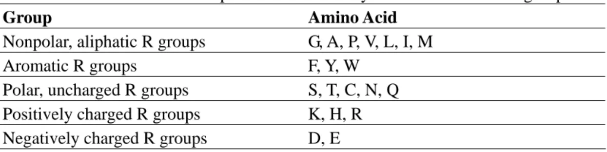
3) The amino acid group: The twenty amino acids are classified into five groups [22], listed in Table 2.3..

Table 2.3. The relationship between the twenty amino acids and five groups

Group Amino Acid

Nonpolar, aliphatic R groups G, A, P, V, L, I, M

Aromatic R groups F, Y, W

Polar, uncharged R groups S, T, C, N, Q

Positively charged R groups K, H, R

Negatively charged R groups D, E

4) The secondary structure of the residue: We could get the secondary structures of the residues in protein complexes from the DSSP file [19].

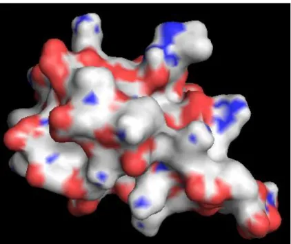
5) The electric charge distribution near the residue (EC): The electric charge near the surfaces is considered because phosphate outside DNA is negative charge carriers. Therefore, we establish the new feature via the influence of charges. A diagram about above-mentioned idea is given in Figure 2.2. And in amino acid, the property with respect to charge is pI value. However, these values must transform into another form for each residues in proteins. The evaluation function of the feature is as follows.

The referenced pI values of the twenty amino acids are sowed in Table 2.4 [22]. Each pI value subtracting five is regard as its electric charge (e.g. the electric value of Glycine is 0.97). This shift process will make that the residues with negative charge have negative value and those with natural charge have near zero.

The electric charge distribution near the residue (EC) is defined as

∑

i represents a certain residue. And in the sequence, i-1 and i+1 show the closest left and right position by i residue, respectively. The equation through accumulation estimates the charge near i residue.

Figure 2.2. An example for electric charge near the surfaces of the residues: The graph shows the atom distribution of the protein surface. Blue and red areas are atoms with positive and negative charge, respectively. We inferred this blue part may bind to DNA. Therefore, we bring up an idea which is to make use of the ASA value of each residue and its pI value for the charge distribution estimation roughly.

Table 2.4. The amino acid and its pI value

Amino Acid pI Amino Acid pI

Glycine 5.97 Serine 5.68 Alanine 6.01 Threonine 5.87 Proline 6.48 Cysteine 5.07 Valine 5.97 Asparagine 5.41 Leucine 5.98 Glutamine 5.65 Isoleucine 6.02 Lysine 9.74 Methionine 5.74 Histidine 7.59 Phenylalanine 5.48 Arginine 10.76 Tyrosine 5.66 Aspartate 2.77 Tryptophan 5.89 Glutamate 3.22

Based on equation (2.1), EC value has the opportunity of being amplified obviously if the i residue lies near the surface of the protein, since we multiply ASA value. And in case of buried completely, EC value is zero. The purpose is to get more distinction by the process. Note that ASA values for the calculation of EC values are gotten by

DSSP program directly, not relative ASA (rASA). We hope EC values are influenced more deeply by these bigger residues with absolute larger surfaces, not those smaller residues with relative larger surfaces. Besides this part, relative ASA is used in other parts in our work.

Chapter 3

Methods

3.1 The proposed decision tree method

Decision tree [7] is a popular machine learning method to classify the value of a discrete dependent variable with a finite set. The basic decision tree example and algorithm[23] are given in Figure 3.1 and 3.2, respectively. Decision tree learning is a method for approximating discrete-valued target functions that is robust to noisy data and capable of learning disjunctive expressions [5]. Learned trees can also be re-represented as sets of if-then rules to improve human readability.

A decision tree is constructed by looking for regularities in data. According to entropy calculation, we can select one with the minimum entropy from these features. Given a collection S, if the target attribute can take on c different values, then the entropy of S relative to this c-wise classification is defined as

i c i i p p S Entropy ₂ 1 log ) (

∑

where pi is the proportion of S belonging to class i [5]. Each level of the trees will be

decided by the rule. The distributions of the levels of the tree are important and readable information because we could analyze which feature is more significant than others [5, 7]. In our wok, C5.0 [24], an update version of C4.5 [25] algorithm, is applied in the proposed decision tree method.

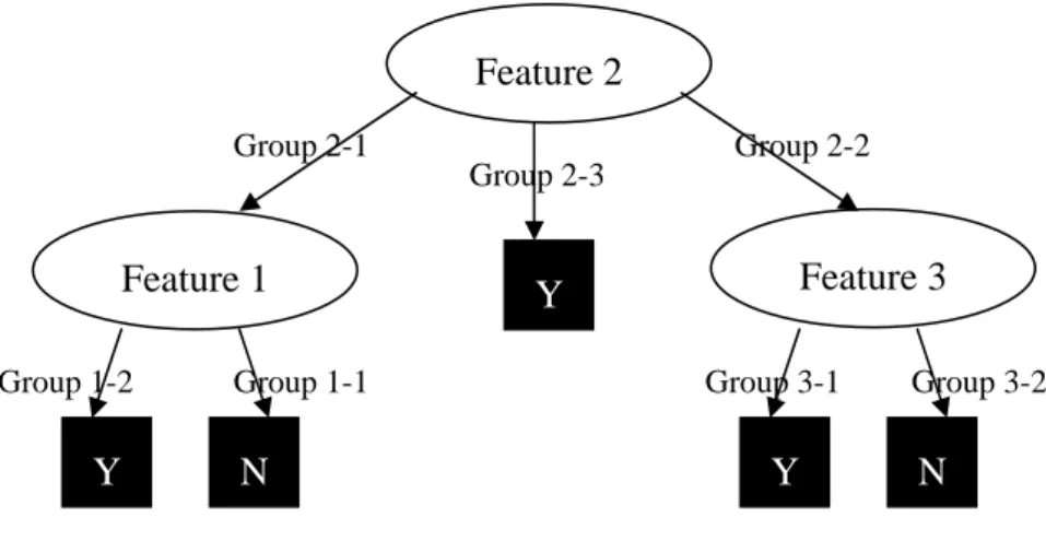
Figure 3.1. An example for decision tree method: A simple is input the system. If its Feature 2 value belongs to Group 2-1, it will leave for Feature 1 node. And then if its Feature 1 value is a portion of Group 1-2, the decision tree system will show it is a member of Class Y. Other classification pathways can be analogized by the above-mentioned mode.

Figure 3.2. The basic decision tree algorithm

Group 3-2

Group 2-1 Group 2-2

Group 2-3

Group 1-2 Group 1-1 Group 3-1

Feature 2

Feature 1 Feature 3

Y N Y N

3.1.1

The Parameters Setting

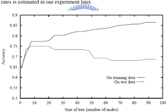
Over-fitting is a significant practical difficulty for the bulk of machine learning methods. Figure 3.3 [5] illustrates the impact of over-fitting in a typical application of decision tree learning. There are two major approaches to avoiding over-fitting in DT. These approaches are to stop growing the tree earlier and post prune [5]. Pruning a decision node consists of removing the sub-tree rooted at that node, making if a leaf node, and assigning it the most common classification of the training examples affiliated that node [5]. To determine the correct final tree size were reported in many researches [26-29]. In this research, we utilize post pruning method [25]. That the pruning parameter, confidence factor (cf), certainly affects the performance about error rates is estimated in our experiment later.

Figure 3.3. Over-fitting in decision tree learning: As DT system adds new nodes to grow the decision tree, the accuracy of the tree measured over the training examples increases monotonically. However, when measured over a set of test examples independent of the training examples, accuracy first increases, then decreases.

As a result of unbalanced distribution of samples, the penalty will be considered to avoid that accuracy about binding ones are sacrificed. The parameter setting is equal to increase the binding influence for the classification results. And it would enhance

NP performance.

Furthermore, the idea of adaptive boosting algorithm [24, 30] to create several decision trees is used in our method. Boosting is a technique for generating and combining multiple classifiers to improve predictive accuracy [24]. When a new case is to be classified, each decision trees vote for its predicted class and the votes are counted to determine the final class. In general, to predict the unknown data by using more decision trees will get a better accuracy than by only using one in our research.

3.1.2

The judgment for the attribute of the features

To select features which have more attribute for classifying example is critical. What is a good quantitative measure of the worth of an attribute? We would define a statistic property that measures how well a given attribute separates the training examples according to their target classification [5]. The best feature choice to build trees generally leads to simple decision at the nodes [6]. A variety of selection attributes measures have been proposed in past researches [31-33]. In the thesis, we would refer three kinds of judgment for the attribute. The source of the part about measuring the attribute comes from [5].

The measure is simply the expected reduction in entropy caused by partitioning the examples according to this attribute. First used judgment function is Information Gain. It is defined as Information Gain(S,A) ( ) | | | | ) ( ) ( v A Value v v S Entropy S S S Entropy

∑

Where Values(A) is the set of all possible values for attribute A, and Sv is the subset of

S for which attribute A has value v. The first term in Equation (3.2) is just the entropy of the original collection S, and the second term is the expected value of the entropy after S is partitioned using attribute A. The expected entropy described by this second term is the sum of the entropies of each subset Sv, weighted by the fraction of

examples | | | | S S_v that belong to Sv.

However, Equation (3.2) has so many possible values that it is bound to separate the training examples into very small subsets. Because of this, it will have a very high information gain relative to the training examples, despite being a very poor predictor of the target function over unseen instances. Therefore, one alternative measure that has been used successfully is the gain ratio [7]. The gain ratio measure by incorporating a term, called Potential Information:

Potential Information(S,A)

∑

where S1 through Sc, are the c subsets of examples resulting from partitioning S by the

c-valued attribute A. And Gain Ratio measure is defined in terms of the earlier Information Gain measure, as well as this Potential Information, as follows

Gain Ratio(S,A) ) 3 . 3 ( ) 2 . 3 ( Equation Equation ≡ (3.4)

In thesis, these features adopted from the dataset can be chiefly ranked by Gain Ratio to prediction. The attributes chosen imply that they own the maximum distinct ability for each split.

3.1.3

Training and Test

The results reported in this thesis mainly show three-fold cross validation (3-CV). It is to say the data are divided into three approximately equal parts. And then, two parts are training data and another is test data by turns. During the training, the nodes of each level in decision tree will be established gradually. And then, the test data are input the system. We could get the first result. Following the process, the three parts take turns the test and training data. On account of using three-fold cross validation, the final results in the thesis are the average of the three times test results.

3.2 Accuracy scores

There are two major evaluations to compare the results in diverse parameter setting in the thesis. First one, total accuracy would supply us with the correct ratios in the

whole. Second, the binding and nonbinding data in DNA-binding protein are unbalanced. If we only consider total accuracy, the classification might decide all data are nonbinding since the nonbinding data are most part. But the prediction will lose its meaning. Consequently, NP value provides suitable comparing standpoint for the unbalanced data in the experiment.

Total accuracy score is the ratios of the number of correct predictions. (T-True, F-False, P-Positive, N-Negative).

% 100 ) ( ) ( × + + + + = FN FP TN TP TN TP accuracy (3.5)

Sensitivity and specificity of the predictions are defined as:

% 100 ) ( + × = FN TP TP y sensitivit (3.6) % 100 ) ( ) ( × + = FP TN TN y specificit (3.7)

Net prediction (NP) is the average of the sensitivity and specificity [4].

2 y specificit y sensitivit NP= + (3.8)

Although total accuracy is certainly judged for the results of predictions, NP value is considered in the discussion of the result because binding and nonbinding data sets are unbalanced in this work. We will get biased outcome if we only though about total accuracy scores.

3.3 The process in the experiment

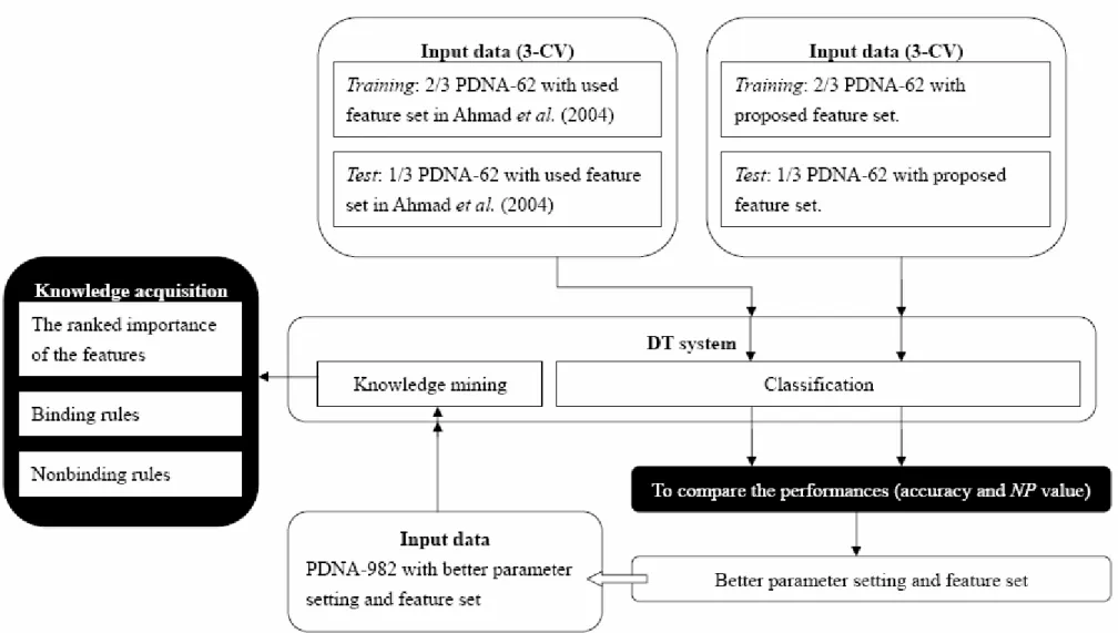
First, the same features with [4] and dataset, PDNA-62, are input DT system. In this process, the used features are the residue, its relative ASA and its two nearest neighbors in the sequence. The models would be considered these regulable parameters, inclusive of boosting, different cf values (the extent of the Pruning) and diverse weights. By the way, we are able to compare simply NN method with DT for the influence of the results at the equal condition.

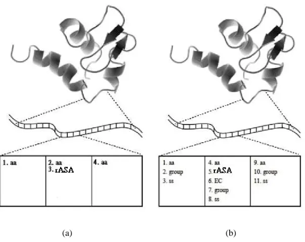
And then, we use PDNA-62 with our proposed features to predict. It means the original features are replaced by new ones, including the residue, its group, secondary structure, relative ASA, EC and its neighbor information. To obtain these original and new feature sets is showed in Figure 3.4. Each vector in the two feature set has 4 and 11 dimensions, respectively, and the decision tree system is sets up via C5.0 model. The model in this part also is used above-mentioned regulable parameters. The performance about the change would easily make the contrast. Thus, we could realize which feature set is better for the DNA-binding protein prediction. Finally, these chosen features will go a step further. A large number of data, PDNA-982, with the proposed features will be utilized to mine knowledge. The framework of the thesis is given in Figure 3.5.

(a) (b)

Figure 3.4. An example for getting the features: The upper level in the figure presents a protein structure. And the middle level shows a portion of the protein sequence. (a) The same feature sets with Ahmad et al. (2004) are displayed. (b) We can obtain the proposed features for each residue. (“aa” means its residue and “ss” indicates its secondary structure).

Chapter 4

Result

4.1 Performance evaluation

4.1.1

Using original feature sets in PDNA-62

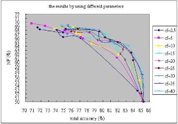
The cf values are considered combining each weight in early work. We want to know the influence of the cf value, and the portion about the research is given in Figure 4.1. Although these lines had similar tendencies, they cause disparity in the results, inclusive of total accuracy, NP value and decision tree size. Generally, the smaller cf values establish the more brief decision trees with readable characteristic. But we should think about the balance of the performance and the tree size. In Figure 4.1, we discover the over-low cf value would make the harmful influence for classifications. However, the influence would progressively decrease when the cf value reach certain rang. Therefore, we choose cf = 20 to do our later research in the thesis.

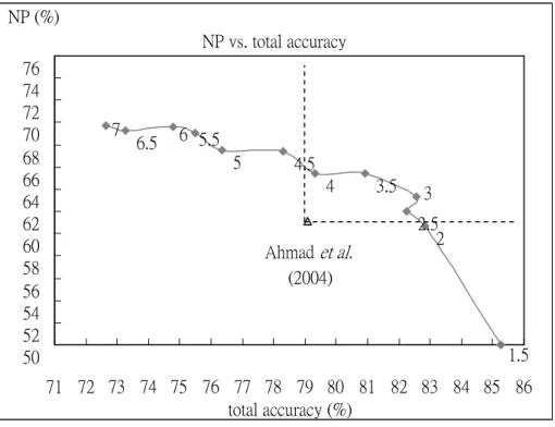
Decision trees are built by the same features with [4] research via C5.0 system. The gray lines in Figure 4.2 showing the performance in this process compare with the conclusion of the original paper, represented by the hollow triangle point. Its NP value is 61.1% and total accuracy is 79.1%. The two performance values of these parts of our results showed in Figure 4.2 are better than this referenced paper, if the gray points lain in the right-up of the hollow point. The left-up portion of the hollow point express that NP value is better than referenced paper, but total accuracy is worse than it. And the mean of the right-down points of the referenced results describe the

Figure 4.1. To compare NP value and total accuracy in different parameters: From right to left in each curve, the weights are gradually increasing.

opposite results to these left-up ones.

We could detect that the added weights would effect the distribution of the results - bigger weights, better NP values. The values near the points show its weight parameters in Figure 4.2. The trees are pruned too seriously when lower weight because the binding are regarded as noises. For these reasons, the bigger weights are considered making the binding data, the less part in the total, rather getting the opportunities of the reserve than eliminating. Nevertheless, the total accuracy value would be sacrifice, because one binding datum which gets the correct classification might cause more mistakes, i.e. more nonbinding data are regarded as noises. For the same thought, using the smaller weights, more nonbinding would be classified correctly; but the binding data would be displayed more wrong classification. Even better total accuracy performance is observed. In according to the NP function, raising the little judgment of the nonbinding data and losing the much one of the binding data in each relative ratio would make NP value decreasing. For the above-mention, we

Figure 4.2. To compare the results between Ahmad et al. (2004) and our proposed method: The gray line use original features, the same with the suggestion in Ahmad et al. (2004) and the weights are showed beside the points. And the hollow triangle point displays the result of Ahmad et al. (2004). The dotted lines purpose to explain conveniently and are unconcerned with the results of the experiment.

could get the appropriate the NP value and the total accuracy if we choose the middle weights. These results with middle weights are given in the right-up of in Figure 4.2.

4.1.2

Using the proposed feature sets in PDNA-62

The black lines in Figure 4.3 show the performance of the proposed 11 dimensions into C5.0. We could get more useful results by using the feature set than the original one. No matter what the NP value or the total accuracy could lie in the greater grade in the black curve in Figure 4.3. According Table 4.1, we are able to analyze the trend. When the bigger weights added, the sensitivity, the ratio of the accuracy prediction of the binding data, would raise. But the process makes the specificity, the ratio of the accuracy prediction of the nonbinding data, diminish. The total accuracy is reducing and the NP value is increasing because the nonbinding data have more part in the whole. NP vs. total accuracy 7 6.5 6 5.5 5 4.5 4 3.5 ₃ 2.5 2 1.5 Ahmad et al. (2004) 50 52 54 56 58 60 62 64 66 68 70 72 74 76 71 72 73 74 75 76 77 78 79 80 81 82 83 84 85 86 total accuracy (%) NP (%)

Figure 4.3. To compare the results in different parameters: The black line expresses the result by using proposed feature set, 11 features, the weights are showed besides the point. Other presentation is the same with Figure 4.2.

Table 4.1. Performance of the different feature sets: When cf = 20, to use the different weights shows the difference between the original and the new feature performance.

the original features the new features

weight

total accuracy (%) NP (%) total accuracy (%) NP (%)

1 85.25 50 84.84 51.29 1.5 85.25 50 85.2 57.82 2 82.84 60.64 84.88 66.42 2.5 82.24 61.99 84.35 69.99 3 82.58 63.33 82.81 71.59 3.5 80.93 65.37 81.05 72.29 4 79.32 65.46 79.72 72.9 4.5 78.29 67.42 78.07 73.3 5 76.36 67.56 76.8 73.3 5.5 75.49 69.09 75.29 73.36 6 74.78 69.61 74.85 73.52 6.5 73.27 69.28 73.15 73.3 7 72.64 69.73 71.91 73.47 NP vs. total accuracy 7 6.5 6 5.5 5 4.5 4 3.5 ₃ 2.5 2 1.5 7 6.5 6 5.5 5 4.5 ₄ 3.5 ₃ 2.5 2 1.5 1 Ahmad et al. (2004) 50 52 54 56 58 60 62 64 66 68 70 72 74 76 71 72 73 74 75 76 77 78 79 80 81 82 83 84 85 86 total accuracy (%) NP (%)

According to above-mentioned performances, we suggest the classification problem should utilize the middle weights, from 2 to 4, and appropriate cf value, near 20. That could provide the suitable results with considered total accuracy, NP value and tree size for proposed 11 features by using DT method. In Figure 4.4, we show the comparison of NP value by the similar total accuracy in the different conditions. The viewpoint is fair and easily observable for realizing the performance. From Figure 4.4, we are aware that DT method can improve the classification results for the same features. And by C5.0 model, the new proposed features provide a serviceable way for predicting DNA-binding proteins.

To compare differnet methods

79.1 61.1 79.32 65.46 79.72 72.9 0 10 20 30 40 50 60 70 80 90 total accuracy NP (% )

Figure 4.4. To compare our result with previous researches: The white bar shows the result of Ahmad et al. (2004). These gray and black bar are our results by using the original and proposed features with cf = 20, weight = 4 in DT method, respectively.

4.2 Knowledge acquisition

In early work, we have proved DT system and new proposed features could get better results. In this part of the thesis, the advanced knowledge acquisition from DNA-binding proteins would be a major purpose. And we hope these data are able to

more creditable for the rules in biological meaning. For the reason, we input PDNA-982, a large number of dataset, to mine knowledge by C5.0 system and the proposed features in this part of the experiment.

4.2.1

The importance order of the features

According to the levels of the trees, the nodes near the roots are more critical for the establishment of the decision tree. To utilize the decision tree system ranks the importance of these features which is listed in Table 4.3. It shows the best attributes and their corresponding values with high gain ratio at each split in the top 3 tree levels.

The table which depends on the degree of the high ratio by the decision trees would help us to understand which features have important influence for the classification. Gain ratio, the ratio of information gain to potential information, is adopted by DT system. For every tree split, this criterion will select an attribute with the highest gain ration. The chosen attributes imply that they own the maximum distinct ability for each split. Features adopted from the dataset could be ranked by the contribution to predict. By Table 4.3, we could acquaint rASA and the new feature, e.g. EC value and its group, really assist in classifying these data.

4.2.2

Rules mining

Once a decision tree model has been constructed, it is a simple and straightforward matter to convert it into an equivalent set of rules by traversing any given path from the root to any leaf. To discover binding and nonbinding rules would supply the readability and understanding of data for humans.

Table 4.4 and 4.5 represent the important rules for non-binding and binding data, respectively. The foundation of the prediction of the decision tree system is observed by these tables. “Size” in these tables means the length of antecedent sentence. And “Support” of one decision rule refers to the proportion of records in the data set that conform to the rule. For an example, the rule1: if EC <= 5.217 from Table 4.4, the

Table 4.2. The ranked importance of proposed features: Best attributes with high gain ratio at each split and their corresponding values

Tree level Attributes Value Potential information Information gain Gain ratio

1 rASA 7.12251 0.857 0.026 0.030 2 rASA 1.27065 0.992 0.010 0.010 2 EC 1.866 0.797 0.014 0.018 3 Group --- 1.264 0.001 0.001 3 rASA 2.897 0.975 0.003 0.003 3 EC -10.891 0.989 0.004 0.004 3 EC 90.847 0.529 0.007 0.013

items of these rules are to explain that 162490 data matched this rule in whole dataset. And then to predict non-binding would get 96.5% in accuracy.

The tendencies about binding and nonbinding rules reveal in Table 4.4 and Table 4.5. We could note the major symbols afterward rASA or EC in Table 4.4 are “<=”, and they are “>” in Table 4.5. We deem these rules fit the fundamental biological knowledge. It means the residues near the surfaces of the proteins with positive charge have more opportunity of binding to DNA, the molecular with negative charge from phosphate. Further, we analyze more information from Table 4.4 and 4.5. These rules also conform to the ranked importance of the attribution in Table 4.3 because rASA and EC value are significant factor for the decision tree to classify.

In Table 4.4, besides the node2 of the rule4, most rules fit the above-mentioned common sense in biochemistry. The rule4 in Table 4.4 means the residues do not prefer to bind to DNA, even these neighbors of the residues having positively charged R groups because of the less surfaces exposed to solvent near the residues.

Table 4.3. The nonbinding rules for DNA-binding proteins: Decision rules with high accuracy and corresponding details for non-binding. (“nbr1_ss” presents the secondary structure of the former neighbor. And “nbr2_aa” shows the residue of the after neighbor. “*” explains nil. The other presentation is analogized.)

Decision rules Size Accuracy Support

if EC <= 5.217 1 96.5 162490

if rASA <= 1.271 1 99.9 66836

if group = Nonpolar, aliphatic R groups and rASA <= 7.835

and nbr1_ss = H

3 99.8 40149

if rASA <= 6.554

and nbr2_group = Positively charged R groups 2 99.3 19718

if aa = L

and rASA <= 47.782 and nbr1_ss = H

Table 4.4. The binding rules for DNA-binding proteins: Decision rules with high accuracy and corresponding details for binding

Decision rules Size Accuracy Support

if ss = *

and group = Aromatic R groups and rASA > 33.772

and nbr1_aa = R

4 83.09 207

if group = Aromatic R groups and rASA > 37.422 and EC > 105.012 3 76.40 267 if aa = I and ss = * and rASA > 1.271 and rASA <= 6.554 and EC > 5.252 and EC <= 12.6

and nbr2_group = Nonpolar, aliphatic R groups

7 73.56 208

if ss = *

and EC > 142.1

and nbr2_group = Polar, uncharged R groups

3 71.84 309 if rASA > 7.123 and rASA <= 43.987 and nbr1_aa = G and nbr2_aa = S and nbr2_ss = H 5 64.19 229

In Table 4.5, we find the aromatic R groups might raise the opportunity of the binding. We reason there are several reasons. First one, the aromatic R groups exits some steric or electronic effects. These effects might cause more attraction with DNA. And another reason, these residues with these groups would be conserved or they are the sections of the domains in DNA-binding proteins. The inference about these reasons will need to do more experiment in biochemistry.

The phenomenon about the cover rate of the data number is extremely discrepant between nonbinding and binding rules. We infer unbalance data and data distribution cause this condition. It is a difficult problem to compact a wide region in data distribution space for only existing binding data except setting up more capable

feature set to learning models. On the contrary, the nonbinding data are major part in the whole. It would easily get higher cover rate and accuracy for the nonbinding rules.

When C5.0 system classifies the total data roughly, i.e. the rule sizes are smaller, it is effortless to read for people. However, this manner would make higher cover rate but lower accuracy. However, this method by more detailed rules, more nodes, not only decrease cover rate but also increase the difficulty to interpret for people. Therefore, we choose certain rang of the pruning value, cf = 20. It causes the binding rules are interpretable and makes the cover rate and accuracy have a certain level.

Chapter 5

Conclusion

DNA-binding protein problem is an essential issue for studying gene regulation. Consequently, it concerns with metabolism and disease occurring in organisms indirectly. In this thesis, an interpretable machine learning method, DT system, and other features are proposed. We hope the entire classification system could achieve a goal, to decrease the cost and time in biochemical experiment.

5.1 DT for DNA-binding protein prediction

According to performance evaluation, the choice about the weights in C5.0 model could provide a different consideration for the score function, total accuracy and NP equation This parameter, weight setting, could give us more elastic for dealing with problems. In general, we suggest the middle weights, nearby 3, be utilized because they would supply the adopted total accuracy and NP value at the same time.

Based the results of the performance, decision tree (DT) system is a better classification than neuron network (NN) for this topic. DT method is effectiveness due to its characteristic, inclusive of the ability of immediate coping with symbol features and higher dimension problem. Furthermore, our new feature set also aids for classifying these data. Therefore, the proposed C5.0 model, using these parameter settings and 11 features, provide a useful classifier to deal with DNA-binding protein prediction problem.

5.2 Knowledge acquisition by DT

After prediction, we further want to obtain the knowledge hidden from DNA-binding proteins. To take advantage of the property, one pathway from the root to its leaf being one rule, in DT system, the significant features and rules would have opportunity to be discovered. A large number of data are obtained in order to get representative knowledge.

The ranked importance of the features and the rules about binding or nonbinding with DNA would supply us with interpretable classifying criterion. Nevertheless, the high cover rate in binding rules is not observed. We refer that phenomenon with respect to the characteristic of these data which involves the distribution of the unbalanced data. Although some knowledge from DNA-binding proteins is acquired, we could not deny that the part in the research have a chance of doing better while new features were added.

5.3 Future work

This research could support the predication of the binding or nonbinding with DNA for these unknown and no significant homology proteins. In future work, besides searching for more useful features, to develop more effective machine learning methods and to do advanced analysis in biochemical experiment will help the research in the field.

Bibliography

[1] D. Lejeune, N. Delsaux, B. Charloteaux, A. Thomas, and R. Brasseur, "Protein-Nucleic Acid Recognition: Statistical Analysis of Atomic Interactions and Influence of DNA Structure," PROTEINS: Structure, Function, and Bioinformatics, vol. 61, pp. 258-271, 2005.

[2] N. M. Luscombe, S. E. Austin, H. M. Berman, and J. M. Thornton, "An overview of the structures of protein-DNA complexes," Genome Biology, vol. 1, pp. 1-10, 2000.

[3] D. Frishman and H. W. Mewes, "PEDANTic genome analysis," Trends in Genetics, vol. 13, pp. 415-416, 1997.

[4] S. Ahmad, M. M. Gromiha, and A. Sarai, "Analysis and prediction of DNA-binding proteins and their binding residues based on composition, sequence and structural information," Bioinformatics, vol. 20, pp. 477-486, 2004.

[5] T. M. Mitchell, Machine Learning: McGraw-Hill, 1997.

[6] R. O. Duda, P. E. Hart, and D. G. Stork, Pattern Classification, 2 ed: Wiley-Interscience, 2000.

[7] J. R. Quinlan, "Induction of decision trees," Machine Learning, vol. 1, pp. 81-106, 1986.

[8] R. Kohavi and J. R. Quinlan, Decision-tree discovery. Handbook of data mining and knowledge discovery. New York: Oxford University Press, 2002. [9] S. Ahmad and A. Sarai, "PSSM-based prediction of DNA binding sites in

proteins," Bmc Bioinformatics, vol. 6, 2005.

DNA-binding proteins using structural motifs and the electrostatic potential," Nucleic Acids Res., vol. 32, pp. 4732-4741, 2004.

[11] N. M. Luscombe and J. M. Thornton, "Protein-DNA interactions: Amino acid conservation and the effects of mutations on binding specificity," Journal of Molecular Biology, vol. 320, pp. 991-1009, 2002.

[12] S. Selvaraj, H. Kono, and A. Sarai, "Specificity of protein-DNA recognition revealed by structure-based potentials: Symmetric/asymmetric and cognate/non-cognate binding," Journal of Molecular Biology, vol. 322, pp. 907-915, 2002.

[13] C. O. Pabo and L. Nekludova, "Geometric analysis and comparison of protein-DNA interfaces: Why is there no simple code for recognition?," Journal of Molecular Biology, vol. 301, pp. 597-624, 2000.

[14] K. Nadassy, S. J. Wodak, and J. Janin, "Structural features of protein-nucleic acid recognition sites," Biochemistry, vol. 38, pp. 1999-2017, 1999.

[15] H. Kono and A. Sarai, "Structure-based prediction of DNA target sites by regulatory proteins," Proteins-Structure Function and Genetics, vol. 35, pp. 114-131, 1999.

[16] R. A. O'Flanagan, G. Paillard, R. Lavery, and A. M. Sengupta, "Non-additivity in protein-DNA-binding.," Bioinformatics, vol. 21, pp. 2254-2263, 2005.

[17] C. O. Pabo and L. Nekludova, "Geometric Analysis and Comparison of Protein-DNA Interfaces: Why is there no Simple Code for Recognition?," Journal of Molecular Biology, vol. 301, pp. 597-624, 2000.

[18] A. Sarai and H. Kono, "Protein-DNA Recognition Patterns and Predictions.," Annual Review of Biophysics and Bimolecular Structure, vol. 34, pp. 379-398, 2005.

[19] W. Kabsch and C. Sander, "Dictionary of protein secondary structure," Biopolymers, vol. 22, pp. 2577-- 2637, 1983.

of solvent accessibility," Bioinformatics, vol. 18, pp. 819-824, 2002.

[21] S. Ahmad, M. M. Gromiha, and A. Sarai, "Real value prediction of solvent accessibility from amino acid sequence," Proteins-Structure Function and Genetics, vol. 50, pp. 629-635, 2003.

[22] D. L. Nelson and C. M.M., Lehninger Principles of Biochemistry, 4 ed. New York: Worth Publisher, 2004.

[23] C. Roach, Building Decision Trees in Python: O'REILLY, 2006. [24] J. R. Quinlan, "See5/C5.0.,"

Software avaible at http://www.rulequest.com/see5-info.html, 2003.

[25] J. R. Quinlan, C4.5: Programs for machine learning. San Francisco: Morgan Kaufmann, 1993.

[26] J. R. Quinlan, "Rule induction with statistical data- a comparsion with mutiple regression.," Journal of the Operational Research Society, vol. 38, pp. 347-352, 1987.

[27] J. R. Quinlan and R. Rivest, Information and Computation, pp. 227-248, 1989.

[28] J. Mingers, "An empirical comparison of pruning methods for decision-tree induction.," Machine Learning, vol. 4, pp. 227-243, 1989.

[29] M. Mehta, J. Rissanen, and R. Agrawal, "MDL-based decision tree pruning.," Proceedings of the First International Conference on Knowledge Discovery and Data Mining, pp. 216-221, 1995.

[30] Y. Freund and R. E. Schapire, "A decision-theoretic generalization of on-line learning and an application to boosting," In Proceedings of the second European Conference on Computational Learning Theory, pp. 23-27, 1995. [31] L. Breiman, J. H. Friedman, R. A. Olshen, and P. J. Stone, Classification and

regression trees.: Wadsworth International Group, 1984.

[32] M. Kearns and Y. Mansour, "On the boosting ability of top-down decision tree learning algorithms.," Proceedings of the 28th ACM Symposium on the Theory of Computing, 1996.

[33] T. G. Dietterich, M. Kearns, and Y. Mansour, "Applying the weak learning framework to understand and improve C4.5. ," Proceedings of the 13th International Conference on Machine Learning, pp. 96-104, 1996.