無線感測網路中認知式擇路協定的跨層設計

國 立 交 通 大 學

電信工程學系

碩 士 論 文

無線感測網路中認知式擇路協定

的跨層設計

Cross-Layer Cognitive Routing in Wireless Sensor

Networks

研究生：許裕彬

指導教授：方凱田

無線感測網路中認知式擇路協定的跨層設計

Cross-Layer Cognitive Routing in Wireless Sensor

Networks

研究生：許裕彬

Student：Yu-Pin Hsu

指導教授：方凱田 Advisor：Kai-Ten Feng

國立交通大學

電信工程學系碩士班

碩士論文

A Thesis

Submitted to Department of Communication Engineering

College of Electrical Engineering and Computer Science

National Chiao Tung University

in partial Fulfillment of the Requirements

for the Degree of

Master

in

Communication Engineering

July 2007

無線感測網路中認知式擇路協定的跨層設計

學生：許裕彬

指導教授：方凱田

國立交通大學電信工程學系碩士班

摘 要

感知無線（cognitive radio，CR）的概念在於強調頻段的有效利用。

在無線感測網路的範疇下，本論文提出了一個“以網路配置向量來協

助的認知式擇路協定＂（CNAR），根據跨層的概念達到更有效率地使

用有限的資源。其中，網路配置向量（NAV）被用來估測頻道的狀態，

結果再應用於封包路徑的選擇。此外，“認知式路徑轉換＂及“降低

連結點的區域性路徑修補＂亦被提出來，進一步地提升 CNAR 的效

能。最後，一個理論上的研討及數個模擬結果將用做性能的評估與比

較。其結果顯示出，在不大量耗費控制封包的情況下，所提出的 CNAR

比現今許多類似的擇路協定表現更佳，特別是在頻道擁塞的情況下，

更能突顯出 CNAR 的優勢。

Cross-Layer Cognitive Routing in Wireless Sensor Networks

Student：Yu-Pin

Hsu

Advisor：Kai-Ten Feng

Department of Communication Engineering

National Chiao Tung University

Abstract

Cognitive Radio (CR) is a paradigm which aims at improving the spectrum

efficiency by means of the prior information and the ability to adapt. In this

thesis, a Cognitive NAV-Assisted Routing (CNAR) algorithm is proposed to

effectively make use of the limited channel resources with a cross-layer

approach. The existing NAV vectors obtained from the RTS/CTS packets are

utilized for the estimation of the channel status around a sensor node. The

routing path is selected based on the channel-free probability along the route

for the transmission of data packets. Moreover, the cognitive path-switching

scheme and the Reduced Hops Local Repair (RHLR) mechanism further

enhance the routing performance of the proposed CNAR algorithm. The

effectiveness of the proposed CNAR protocol is evaluated via both the

analytical study and the simulation results. Without consuming excessive

power for each sensor node, the CNAR algorithm can achieve better

performance comparing with other existing schemes, especially under the

scenarios with the channel congestion.

誌 謝

首先要感謝指導教授方凱田老師，於研究上提供許多的不同的見

解，以及在文章的表逹方式上給予大力的協助；同時也感謝交大電信

王蒞君老師及交大資工趙禧綠老師於口試時提供了寶貴的建議，更能

促使未來的研究愈臻周全。

接著感謝我的家人，忍受著兒子一年回家沒幾次的難過之餘，還

總是適時地鼓勵；有了他們的支持，讓我更能專心於新竹唸書與研

究。接著，不論是實驗室的同學、球隊上的朋友、大學同學、高中同

學、還是室友們．．．．．．在單調的碩班生活中，是你們增添了我

的生活色彩。

最後，要特別感謝女朋友宜靜。在碩班的生活中，時常在課業與

研究上花了不少時間；謝謝妳的體諒，給我充分的時間應用，同時也

陪伴著我，不斷地鼓勵我。雖然妳有時會發點小脾氣，不過還是很可

愛。另，要感謝宜靜的媽媽，謝謝阿姨在這段時間內的照顧。

我要把這兩年內的小小成果，歸功於一路上陪伴著我的你們，謝

謝你們。各位親愛的，我畢業囉！接下來你們加油吧。

許裕彬謹誌 于交通大學

Contents

1 Introduction 6

2 Preliminaries 9

2.1 The Related Routing Algorithms . . . 9

2.1.1 Ad Hoc On-Demand Vector (AODV) Protocol . . . 9

2.1.2 Load-Balanced Ad Hoc Routing (LBAR) Protocol . . . 11

2.2 The IEEE 802.11 MAC Protocol . . . 11

2.2.1 Distributed Coordination Function . . . 12

2.2.2 Hidden Terminal Problem . . . 12

2.3 The Radio Propagation Models . . . 14

2.3.1 Free Space Model . . . 14

2.3.2 Two-Ray Reflection Model . . . 14

3 The Proposed Cognitive NAV-Assisted Routing (CNAR) Protocol 17 3.1 Channel-free Probability of the Considered Path (Pcf,p) . . . 19

3.2 Route Discovery Process and Cognitive Path-Switching Scheme . . . 22

3.3 Reduced Hops Local Repair (RHLR) . . . 24

3.4 Determination of the Time Interval ∆T . . . 25

4 Analytical Study on the Effects from Data Rate and Neighbor Interference 28 4.1 Analytical Modeling of the IEEE 802.11 Protocol . . . 29

5 Performance Comparison and Evaluation 39 5.1 The Grid Topology . . . 39 5.2 The Random Topology . . . 41

List of Figures

2.1 The Schematic Diagram of the AODV Protocol . . . 10

2.2 The Medium Access Mechanism in DCF . . . 12

2.3 Hidden Terminal Problem . . . 13

2.4 RTS/CTS Scheme in IEEE 802.11 . . . 13

2.5 The Free Space Propagation Model . . . 15

2.6 The Two-Ray Reflection Propagation Model . . . 15

3.1 The Schematic Diagram of the Example Network Topology . . . 18

3.2 The Schematic Diagram of the RTS/CTS Scheme Associated with the NAV Vectors . . . 20

3.3 The Schematic Diagram for the Route Repair Schemes . . . 25

3.4 The Relationship Between the Expected Value of X (i.e. mb) and the Required Number of Samples n . . . 27

4.1 The Embedded Markov Chain Model for IEEE 802.11 Backoff Mechanism . . . 29

4.2 Service Time (Tsv) vs. Data Rate (λ) . . . 35

4.3 Service Time (Tsv) vs. Number of Interfering Neighbors (α) . . . 35

4.4 Packet Delivery Ratio vs. Data Rate λ (Solid Lines: Analytical Results; Dashed Lines: Simulation Results) . . . 38

4.5 Packet Delivery Ratio vs. Number of Interfering Neighbors α (Solid Lines: Analytical Results; Dashed Lines: Simulation Results) . . . 38

5.1 Simulation Result of the Grid Topology : Packet Delivery Ratio vs. Data Rate of R3 . . . 43

5.2 Simulation Result of the Grid Topology : Average End-to-End Delay vs. Data Rate of R3 . . . 43

5.3 Simulation Result of the Grid Topology : Power Consumption from Control Overhead vs. Data Rate of R3 . . . 44

5.4 Simulation Result of Random Topology : Packet Delivery Ratio vs. Number of Sources . . . 44 5.5 Simulation Result of Random Topology : Average End-to-End Delay vs.

Num-ber of Sources . . . 45 5.6 Simulation Result of Random Topology : Power Consumption from Control

Overhead vs. Number of Source . . . 45 5.7 Simulation Result of Random Topology : Packet Delivery Ratio vs. Average

Data Rate . . . 46 5.8 Simulation Result of Random Topology : Average End-to-End Delay vs.

Av-erage Data Rate . . . 46 5.9 Simulation Result of Random Topology : Power Consumption from Control

List of Tables

4.1 Analytical and Simulation Parameters Adopted from the DSSS System . . . 34 5.1 Simulation Parameters for the Grid Topology . . . 40 5.2 Simulation Parameters for the Random Topology . . . 42

Chapter 1

Introduction

The Wireless Sensor Network (WSN) has attracted a significant amount of attention in re-cent years. A WSN consists of Sensor Nodes (SNs) that can cooperatively perform different tasks, including monitoring, locating, and data distribution/aggregation [1] - [4]. Due to the distributed nature and hardware cost associated with the SNs, the available resources (espe-cially the battery power) are considered limited for most of the current applications. How to provide efficient energy conservation for the SNs has become an important issue for the design of the WSNs. The Cognitive Radio (CR) technology [5] - [9], which provides dynamic channel adjustment, can be employed to maximize the utilization of the available resources. The adaptive self-learning process within the CR technique can be considered as a feasible approach in the protocol design for the WSNs. The adoption of the CR technology has been revealed under different communication layers [5] - [7]. The cognitive process, spectrum man-agement, and several CR applications are proposed as in [5] from the PHY layer point of view. A MAC layer scheduling, which exploits an Integer Linear Programming, was presented in [6]. A network layer CR algorithm was investigated in [7] in order to provide better end-to-end performance by the cognitive process. In this thesis, a CR-based network layer protocol will be proposed by adopting the available MAC layer information for the WSNs.

A feasible design of multi-hop routing protocol within the power-constrained environments is considered an important topic for the WSNs. Different types of routing protocols have been

developed, which can be categorized into proactive (e.g. DSDV [10]) and reactive algorithms (e.g. AODV [11] and DSR [12]). However, these protocols may lead to poor routing perfor-mance (e.g. low packet delivery ratio and high end-to-end delay) due to the channel congestion within certain area of the WSN. As some of the SNs in the network are exhaustively utilized, the rapid power consumption and failure of these SNs may result in unreliable communica-tion linkages. Therefore, it will be difficult to guarantee persistent routing performance or Quality-of-Service (QoS) within the WSNs. Several congestion control schemes have been investigated [13] - [16] to improve the multi-hop routing performance. The Dynamic Code-word Routing (DCR) [13] proposed a codeCode-word conceptual model to balance the total traffic load within the network. The Load-Balanced Ad Hoc Routing (LBAR) [14] and the Dynamic Load-Aware Routing (DLAR) [15] schemes consider the number of interfering routes around the SN in order to determine if the SN should be selected as a forwarding node within the route. The routing with Minimum Contention time and Load balancing (MCL) [16] algorithm determines its route selection criterion based on the total number of contenting nodes around the neighborhood of a SN, which improves the routing performance with the occurrence of the channel congestion. However, these routing protocols inevitably result in a great amount of control packets for the purpose of alleviating the channel congestion problem. Moreover, the degraded routing performance caused by the variation of the data rates/sizes has not been considered in the previous works.

In this thesis, a Cognitive NAV-Assisted Routing (CNAR) protocol is proposed to alle-viate the channel congestion based on the cross-layer information. The objective of the CR technology can therefore be achieved by preventing the inefficient transmissions under the environments with finite channel resources. Instead of generating control packets to obtain the desired information from the network neighbors, the CNAR scheme utilizes the existing information, i.e. the Network Allocation Vector (NAV), from the Request-To-Send (RTS) and the Clear-to-Send (CTS) packets within the MAC layer. The channel-free probability, which is computed from the NAV vectors of the SN, is carried within the route discovery processes to determine the feasible route for packet delivery. It is noticed that the information inherently

considers different data rates/sizes and the number of interfering neighbors that may occur within the various routes. The proposed CNAR scheme can also cognitively switch between the selected paths while the level of channel congestion has been changed. Moreover, a Re-duced Hops Local Repair (RHLR) scheme is employed within the CNAR algorithm, which can reconnect the broken communication links with reduced number of forwarding SNs. The CNAR scheme can improve the channel congestion problem without the extravagant usage of control packets. The effectiveness of the CNAR algorithm will be validated via both the analytical study and the simulation results.

The rest of this thesis is organized as follows. Chapter 2 briefly reviews several prelimi-naries and related works. The proposed CNAR scheme is explained in Chapter 3. Chapter 4 provides the analytical analysis of the network performance. The performance evaluation of the CNAR scheme via simulations is illustrated in Chapter 5. Chapter 6 draws the conclu-sions.

Chapter 2

Preliminaries

In order to facilitate the design of the proposed CNAR algorithm, the related routing al-gorithms, the IEEE 802.11 MAC protocol, and the radio propagation models are briefly summarized as follows.

2.1

The Related Routing Algorithms

In the computer network, the term routing refers to the path selection along which to send data. Moreover, some metrics (e.g. shortest path, power consumption and minimum inter-ference) can be taken into consideration for the path selection among all possible routes. In this section, two routing protocols, the Ad Hoc On-Demand Vector (AODV) and the Load-Balanced Ad Hoc Routing (LBAR) algorithms, are briefly reviewed. The two schemes will also be implemented in the simulations for performance comparison.

2.1.1 Ad Hoc On-Demand Vector (AODV) Protocol

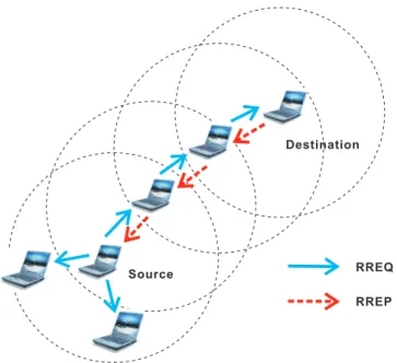
The Ad Hoc On Demand Distance Vector (AODV) [11] routing algorithm is an on demand algorithm that a route discovery, which is complete by a route request/repley cycle as in Fig. 2.1, is initiated only as desired by the source node. When a source node intends to send data to a destination but has no available route, it broadcasts a route request (RREQ) packet throughout the network. Once receiving a RREQ packet, the node will update the

RREQ

RREP Source

Destination

Figure 2.1: The Schematic Diagram of the AODV Protocol

corresponding information about the source node. Besides, it will generate a route reply (RREP) packet, unicasting back to the source node, if either the destination is itself or a route to the requested destination exists; otherwise, it just forwards the RREQ packet. The sequence number, another information in a RREQ packet, is exploited to ensure the freshness of routes and to prevent the loop. As soon as receiving a RREQ packet, the source will start the data transmission. However, if the source later receives another RREP packet containing a greater sequence number or the same sequence number with a smaller hopcounts, it may update its routing information and switch to the better route.

Because of the unstable wireless network environment, the route maintenance is important in the multihop wireless network. Regarding the AODV scheme, if a active route breaks, the upstream node propagates a route error (RERR) packet back to notify the source node of the unreachable destination. After receiving the RERR, the source node will reconstruct a new route to the desired destination.

2.1.2 Load-Balanced Ad Hoc Routing (LBAR) Protocol

Because the AODV takes the shortest path into account, a traffic jam may occur somewhere and lead to the unreliable links. To improve the routing performance, the Load-Balanced Ad Hoc Routing (LBAR) scheme [14] is proposed for delay-sensitive/throughput-sensitive appli-cations. Hence, the LBAR focuses on how to find a path with the minor traffic interference.

The LBAR is also an on-demand algorithm, which conducts the RREQ/RREP cycles for route discovery. The path cost, which considers the number of interfering paths around the forwarding SN, is carried along with the RREQ packets in the LBAR scheme. An appropriate path is selected by the destination node with minimum cost, which is defined as

Ω_κ =X

i∈κ

(ω_i+ ζ_i) (2.1) where Ωκ denotes the cost along the path κ; ωi is the number of active paths through node

i, where i represents a SN on the path κ. ζi indicates the traffic interference as ζi =

P

∀jωji,

which is the activity sum of the neighbors around node i. It is noted that ωi

j denotes the

active paths at node j, which is a neighbor SN of node i.

Merit as the LBAR has, it adopts additional hello packets for the exchange of ω_i, which will foreseeable to induce excessive control packets and speed the power exhaustion. Moreover, the LBAR just considers the number of interference paths as the criterion of route selection, but some important metrics are not in consideration. One of the purpose of the proposed CNAR is to ameliorate the LBAR from some useful information provided by the MAC layer.

2.2

The IEEE 802.11 MAC Protocol

Different types of MAC protocols are exploited within the design of the WSNs [17] - [20] (e.g. the IEEE 802.11 [17] and the S-MAC [18] schemes). In this thesis, the 802.11 MAC protocol is employed owing to its well-adopted capability for collision avoidance.

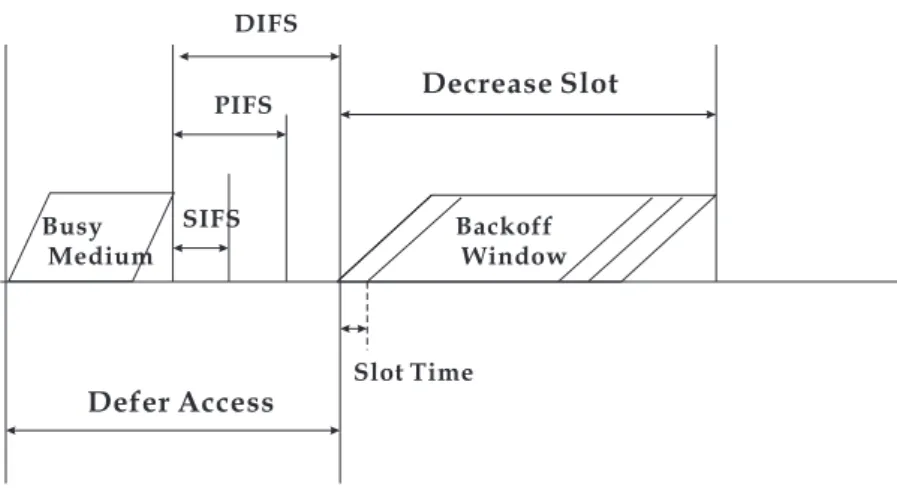
Defer Access Decrease Slot Busy Medium Backoff Window SIFS PIFS DIFS Slot Time

Figure 2.2: The Medium Access Mechanism in DCF

2.2.1 Distributed Coordination Function

The Distributed Coordination Function (DCF) is a basic access mechanism utilized by the MAC protocol in the IEEE 802.11. The DCF is based on a Carrier Sense Multiple Access (CSMA) with Collision Avoidance (CA), which guarantees each SN has a fair chance to access the medium. When adapting CSMA/CA, each SN must sense the medium before its data transmissions. Moreover, the random backoff process is excused in the CSMA/CA to decrease the probability of data collision. As show in Fig. 2.2, before the data transmission, each SN randomly selects the time slots from [0, CW ] to count down, where the CW is the maximum backoff window, and then detects the medium status once the backoff timer expires. However, for fear of choosing the same backoff time slots by the neighbors, the binary exponential backoff algorithm is accompanied to further avoid data collisions.

2.2.2 Hidden Terminal Problem

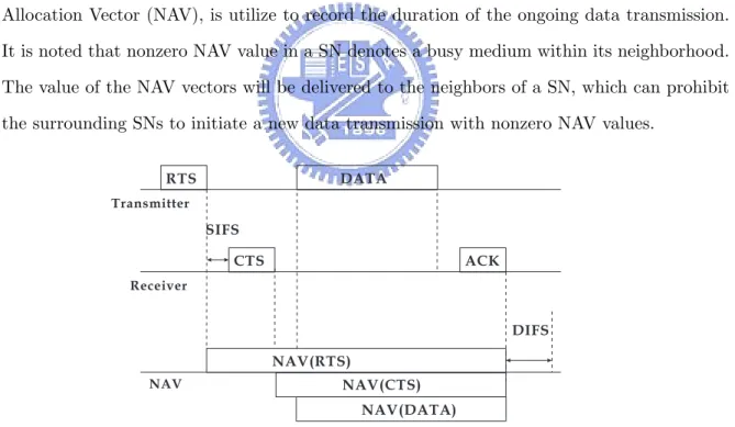
Owing to the limited transmission range, the CSMA scheme can not detect the data transmis-sion that are out of the sense range, which causes the hidden terminal problem as in Fig. 2.3. The hidden node problem will result in the degradation of performance. As illustrated in Fig. 2.4, the optional RTS/CTS exchange before a data transmission is exploited to resolve the potential hidden terminal problem. Furthermore, in order to avoid data collision during the data transmission, the virtual carrier sensing mechanism, which is carried out by the Network

collision

Figure 2.3: Hidden Terminal Problem

Allocation Vector (NAV), is utilize to record the duration of the ongoing data transmission. It is noted that nonzero NAV value in a SN denotes a busy medium within its neighborhood. The value of the NAV vectors will be delivered to the neighbors of a SN, which can prohibit the surrounding SNs to initiate a new data transmission with nonzero NAV values.

RTS CTS DATA ACK NAV(RTS) NAV(CTS) Transmitter Receiver NAV SIFS DIFS NAV(DATA)

2.3

The Radio Propagation Models

The radio propagation models are used to calculate the received signal power of each packet. As a receiving threshold resides in the physical layer, a packet will be marked as error and dropped by the MAC layer if the received power does not reach the predefined threshold; On the contrary, the packet will be passed to the upper layer. This section describes some radio propagation models implemented in Network Simulation (ns-2, [21]).

2.3.1 Free Space Model

The free space propagation model is an ideal condition assuming that there is only the Line-Of-Sight (LOS) path between the transmitter and the receiver. It basically represents the communication range as a circle around the transmitter as in Fig. 2.5. If a receiver is within the circle, the packets is received successful; otherwise, the packets will lose. (2.2) represents the received signal power in the free space at distance d from the transmitter [22].

Pr(d) = PtGtGrλ

2

(4π)2_d2_L (2.2)

where Ptis the transmitted signal power. Gtand Gr respectively represent the antenna gains

of the transmitter and the receiver. L (L ≥ 1) is the system loss, and λ is the wavelength.

2.3.2 Two-Ray Reflection Model

A single LOS path between two station is seldom the only propagation path; more propagation paths is more reasonable. The two-ray-reflection model considers both direct and ground reflection path as in Fig. 2.6, and more accurately predicts the propagation model at the longer distance than the free space model. (2.3) represents the received signal power at distance d [23].

Pr(t) = PtGtGrh

2

th2r

d4_L (2.3)

Figure 2.5: The Free Space Propagation Model

However, the two-ray reflection model does not perfectly perform at a short distance owing to the oscillation caused by the constructive and destructive combination of the two rays. Hence, a cross-over distance dc is given in this model. (2.2) is used when d < dc;

otherwise, (2.3) is used. The same result of (2.2) and (2.3) at the cross-distance will lead to

dc being calculated as

d_c= 4πhthr

Chapter 3

The Proposed Cognitive

NAV-Assisted Routing (CNAR)

Protocol

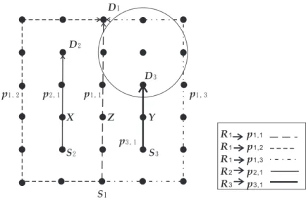
The main objective of the proposed CNAR algorithm is to attain the goal of the CR technology such as to effectively utilize the limited channel resources. The proposed scheme can alleviate the channel congestion problem without the excessive usage of control packets. The CNAR protocol is explained with the network topology as shown in Fig. 3.1. A terminology is defined as Ri ≡ {Si, Di, υi, {pi,j}}, which denotes the ith route with its distinct source

node Si, destination node Di, and the pre-specified data rate υi. Moreover, pi,j indicates

the jth _{path which belongs to the i}th _{route. As shown in Fig. 3.1, there are three routes}

that are denoted as R1 = {S1, D1, υ1, {p1,1, p1,2, p1,3}}, R2 = {S2, D2, υ2, {p2,1}}, and

R3 = {S3, D3, υ3, {p3,1}}. It is noted that the transmission range of each SN encompasses

its one-hop neighborhood as shown in Fig. 3.1.

The following example illustrates the design concept of the proposed CNAR algorithm. Assuming that R₂ and R₃ are the two existing routes for their corresponding data trans-mission, with data rates υ₂ and υ₃ respectively. The source node S₁ intends to transmit data packets to D1. Without the mechanism for congestion control, the conventional AODV

R1 p R p R p R p R p 1,1 1 1,2 1 1,3 2 2,1 3 3,1 D1 S1 S2 S3 D2 D3 X Z Y p1 , 2 p2 , 1 p1 , 1 p3 , 1 p1 , 3

Figure 3.1: The Schematic Diagram of the Example Network Topology

protocol will construct the p_1,1 path for packet delivery (i.e. with the shortest path), which results in severely degraded performance due to the channel congestion (i.e. packet collision) from both routes R2 and R3. The LBAR algorithm, on the other hand, will select p1,3 for

packet delivery since p_1,3 is determined to have the smallest cost Ωp1,3 (as defined in (2.1))

comparing with p_1,1 and p_1,2. However, both (i) the excessive control packets are required to computed the cost function and (ii) the various data rates along different paths are not considered in the LBAR scheme.

Due to the different applications and the Quality-of-Service (QoS) requirements, the data rates υ2 and υ3 associated with the routes R2 and R3 may not be considered to have the

same value. By adopting the CNAR algorithm, the path selected for the route R1 may differ

due to the various data rates that are possessed by its interfering neighbor SNs. As υ2 > υ3

or υ2 ≈ υ3, the path p1,3 will be chosen owing to its least number of interfering neighbor

SNs. On the other hand, the path p_1,2 can be selected while υ2 is comparably smaller than

υ3. Even though p1,3 has smaller interfering neighbor SNs, the high data rate associated with

R3 can result in more severe packet collisions to the path p1,3. This reveals one of the main

objectives of the proposed CNAR protocol as to select the routing path by considering the effects from both the data rate and the interfering neighbor SNs. Moreover, the cognitive

path-switching scheme within the CNAR algorithm will adaptively change the routing path back to p_1,1 while its interference is considered lower than the current transmitting path p_1,2 or p_1,3, e.g. in the case that the data transmissions within R2 and/or R3 are expired. The

cognitive scheme can alleviate the prolonged end-to-end delay (due to larger hop counts) that commonly occurred in the congestion-based routing algorithms. The details of the proposed CNAR protocol are explained as follows.

3.1

Channel-free Probability of the Considered Path (P

)

The channel-free probability is utilized as the criterion for path selection. The value recorded within the NAV vector is exploited to determine the channel idle probability. It is noticed that the NAV vectors within a SN are employed to indicate if the channel is busy with packet transmission. There are four NAV values in each SN that are updated by the RTS packet (Nr), the CTS packet (Nc), the data packet (Nd), and the ACK packet (Na). Each value

represents the remaining time duration until the corresponding data packet has finished its transmission. A SN is considered to possess idle channel status as all its NAV vectors become zero. Since (i) the NAV value set by the data packet generally overlaps with that determined from the RTS packet and (ii) the NAV value determined by the ACK packet is zero in the common non-fragmentation schemes [17], their effects on the channel status are neglected in this thesis.

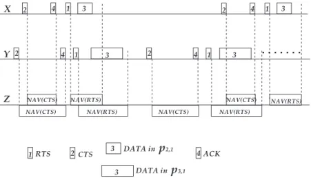
Fig. 3.2 illustrates the timelines for nodes X, Y , and Z (in Fig. 3.1) adopting the RTS/CTS scheme with their associated NAV vectors. It is assumed that node X represents an intermediate node within p_2,1; while node Y belongs to the path p_3,1 for packet transmission. It is also considered that smaller data rate and data size are employed in node X in comparison with that in node Y (as shown in Fig. 3.2). The packets (including the RTS, CTS, data, and ACK packets) “sending” from both nodes X and Y are illustrated in their timelines respectively. Noted that it is required for nodes X and Y to receive the RTS packets from their source node, S2 and S3, in order to send out the associated CTS packets as in Fig. 3.2.

X Y Z 2 1 3 2 1 3 4 4 NAV(CTS) NAV(CTS) NAV(RTS) NAV(RTS) 1RTS 2CTS 3 DATA inp2,1 4ACK 3 DATA in p3,1 2 4 1 3 2 4 1 3 NAV(CTS) NAV(CTS) NAV(RTS) NAV(RTS)

Figure 3.2: The Schematic Diagram of the RTS/CTS Scheme Associated with the NAV Vectors

resides within the communication ranges of nodes X and Y , will consequently be assigned with various NAV vectors due to the packet transmissions from both nodes. The combined NAV vectors within node Z are shown in Fig. 3.2. It can be observed that the accumulated NAV vectors at node Z implicitly contain the mixed effects from both the data rate and the data size of the transmitted packets, i.e. node X with smaller data rate and size comparing with that from node Y .

It is assumed that Ti

Nr(∆T ) represents the time instant that falls within the time duration

created by the ith _{NAV vector from the RTS packet: T}i

Nr(∆T ) = {t ∈ R+| tis,Nr ≤ t ≤

ti

e,Nr, ∀ tis,Nr, tie,Nr ∈ ∆T }, where tis,Nr and tie,Nr denote the starting and the ending time

instants of the ith _N

r vector; and ∆T is the total time interval in consideration. Similarly,

the time instant within the time duration created by the ith_{NAV vector from the CTS packet}

is represented as T_Nci (∆T ) = {t ∈ R+| ti_s,Nc ≤ t ≤ t_e,Nci , ∀ ti_s,Nc, ti_e,Nc ∈ ∆T }, where ti_s,Nc and

ti_e,Nc are the starting and the ending time instants of the ith Ncvector. The set with all the

time instants that fall within the union of the two defined sets can be represented as

TNr(∆T ) ∪ TNc(∆T )

where p and q denote the total number of the NAV vectors defined by the RTS and the CTS packets within the time interval ∆T . The reason for taking the union set of Ti

Nr(∆T ) and

T_Ncj (∆T ) can be observed as in Fig. 3.2. It can be seen that different situations can occur within the network due to the packet contention, e.g. overlapped Nr and Nc, or stand alone

Nc. From the definition of (3.1), the channel-busy probability of a node k can be represented

as

P_b,k= TNr(∆T ) ∪ TNc(∆T )

∆T (3.2)

The probability Pb,k represents an average effect of busy channel for node k within the time

span ∆T . It is worthwhile to notice that the channel busy probability Pb,kinherently combines

the effects from (i) the data rate and data size of the transmitted packets and (ii) the number of the interfering neighbor SNs. For instance, the longer duration obtained from the ith _N

r

indicates that its corresponding data packet has a larger data size to be transmitted; while the number of the interfering SNs and the data rate for a specific set of data packets depending on the occurring frequency of their Nrs (or Ncs) within the time interval ∆T . Therefore, the

channel idle probability for node k becomes

P_i,k = 1 − P_b,k (3.3) It is considered that p is defined as a constructed path with N nodes from the source SN to the destination SN, i.e. p = {1, . . . , k, . . . , N }. In the proposed CNAR scheme, the criterion for the determination of the routing path, i.e. the channel-free probability of the path p (Pcf,p), is defined as

Pcf,p , N −1_Y

k=2

Pi,k = Pi,2· · · Pi,k· · · Pi,N −1 (3.4)

It is noticed that the channel idle probabilities of the source SN (i.e. Pi,1) and the destination

source/destination pair. The processes for acquiring the probability P_cf,p from each SN within the path p will be explained in the next section; while the determination of the time duration ∆T for convergent channel-busy probability P_b,kwill also be addressed in the Section 3.4. The effective utilization of the limited channel resources, i.e. the resources are devoted to successful packet transmissions, can be attained without the excessive usage of the control packets.

3.2

Route Discovery Process and Cognitive Path-Switching

Scheme

The route discovery process of the proposed CNAR scheme is enhanced from the AODV routing protocol. Each node k within the CNAR algorithm maintains a routing table, which contains (i) the next hopping node, (ii) the next two-hopping node, (iii) the sequence num-ber, (iv) the hop counts (HC), and (v) the channel-free probability Pcf,p. It is noted the

information of the next two-hopping node is exploited in the RHLR scheme, which will be discussed in the next section.

As shown in Fig. 3.1, the source node S1 intends to send data packets to the destination

node D1 via some of the forwarding nodes. S1 will first check its route cache to verify

if there are existing paths to D1. If there is no such path in the cache, S1 will start a

route discovery process by broadcasting a route request (RREQ) packet. The channel-free probability Pcf,p will also be recorded within the header of the RREQ packet. It is noted

that Pcf,p1,j represents the probability that the channel along the considered path p1,j is free

to be utilized. Upon receiving the RREQ packet, the intermediate node will multiply its own channel idle probability P_i,k (which is obtained from its MAC layer protocol) to P_cf,p1,j in order to update the channel-free probability along the path p_1,j, i.e. P_{cf, p1,j} = P_{cf, p1,j} · P_i,k. The RREQ packet will be rebroadcasted if the path to the destination node is not available. Until D1 is found in the route discovery process, the first route reply (RREP) packet will be

initiated by D1, and will be sent back to S1 via the reverse path, i.e. via the shortest path

via the RREQ packets. It will also be delivered back to S₁ within the RREP packet via the reverse path p_1,1.

Moreover, at the time instant that the first RREQ packet has arrived in D1, a timer will

be initiated by the destination node D1. As the timer expires, an additional RREP packet

initiated by D1 to S1 is allowed in the CNAR algorithm, i.e. two reverse paths between the

same source/destination pair. The criterion for sending the additional RREP packet from

D1 holds if one of the latter paths (i.e. either p1,2 or p1,3 in the example case) has a larger

channel-free probability comparing with the first path p_1,1, i.e. max

∀ s6=1{Pcf, p1,s} > Pcf, p1,1 (3.5)

As a result, the destination node D1will select either the path p1,2or p1,3 depending on their

channel-free probability values as in (3.4). For discussion purpose, it is considered that the

p_1,2 is selected as the second path due to its larger P_{cf, p1,2} value.

The source node S1 first utilizes the constructed path (i.e. via p1,1) to initiate data

transmission to D1; while the second path (i.e. p1,2) will also be established. In general,

the RREP packet via the path p_1,2 will arrive in S1 in a latter time owing to the larger hop

counts in the path (as shown in Fig. 3.1). S1will consequently change its data delivering path

from p_1,1 to p_1,2 in order to conserve the limited channel resources along the path p_1,1, i.e. channel congestion due to the packet collisions. Furthermore, a control message, the Channel Congestion Level Test (CONG TEST) packet, will also be initiated by S₁ towards the first path p_1,1to determine if the congestion problem along p_1,1has been resolved, e.g. in the case that the data transmissions within R2 and/or R3 have been terminated. The CONG TEST

message, which contains the value of P_{cf, p1,2} within its packet header, will be delivered along the path p_1,1. A criterion is verified at each node k within the path p_1,1 to compare if its own channel idle probability (Pi,k) is greater than the threshold within the CONG TEST message

as P_i,k ≥ ³ P_{cf, p1,2} ´ 1 (HCp1,1 −1) _(3.6)

where HC_p1,1 represents the total hop counts along the path p_1,1. If the condition on (3.6) is satisfied, the CONG TEST message will be carried to the next hopping node along the path

p_1,1. After the message has arrived in D1, it will be traversed back to S1, which guarantees

the resolution of the congestion problem along the path p_1,1. The data transmission from S1

will be cognitively switched back to the path p_1,1, which at present is considered to be the path that has the lowered channel congestion with the smallest hop counts. Moreover, due of the limited numbers of the constructed route within the network, only a slight amount of control packets will be incurred by the CONG TEST messages.

3.3

Reduced Hops Local Repair (RHLR)

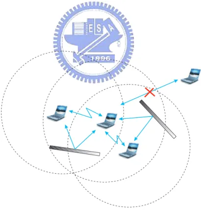
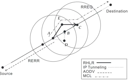
Route repair mechanism is required for multi-hop routing schemes since the communication links can be broken due to many factors, e.g. power exhaustion or unexpected shutdown of the SNs. Fig. 3.3 illustrates the route repair schemes that are utilized in different protocols. It is assumed that the communication link is broken between nodes A and B. The conventional AODV protocol utilizes the route error (RERR) packet for route repair. As node A loses connectivity to its next hop, node A will initiate an RERR packet back to the source node to restart a new route discovery process. Local route repair scheme is adopted in the MCL protocol [16], where node A will initiate a new route discovery process towards the unreachable destination (i.e. by sending the RREQ packet as shown in Fig. 3.3). As can be expected, significant transmission delay can be observed with these two route repair schemes. The IP tunneling is exploited in [24] to construct a new route between nodes A and B. As a consequence, an additional hop count is expected (i.e. via node D) in order to reconnect nodes A and B. It can also be predicted that the hop counts can be drastically increased due to excessively unreliable communication links, i.e. caused by severe packet collision.

The RHLR scheme employed in the proposed CNAR algorithm can further reduce the total hop counts for the local repair. As the link between nodes A and B are broken, node

A will begin a new route discovery process towards both nodes B and C. It is noticed that

RERR RREQ RHLR IP Tunneling AODV MCL Source Destination A B C D E

Figure 3.3: The Schematic Diagram for the Route Repair Schemes

table of a SN. Node A will select the reconstructed local path with the smallest total hop counts. For example, two paths are obtained by node A as {A, E, C} and {A, D, B, C}. It is clear that the path {A, E, C} will be selected by node A since it has comparably smaller hop counts. Due to the localized behavior of the RHLR scheme, the difference on the channel status is observed to be insignificant between the adjacent SNs. Therefore, the channel-free probability (i.e. Pcf,p in (3.4)) will not be considered in the RHLR route selection criterion.

3.4

Determination of the Time Interval ∆T

The determination of a feasible time interval ∆T within the channel-busy probability P_b,k(as in (3.2)) is described in this section. In the IEEE 802.11 protocol, the time scale is slotted with the slot time length denoted as σ, which is set equal to the time required for a SN to detect the transmission of a packet from its neighbor SNs. The σ value depends on the PHY layer design, e.g. σ = 20 µs in the Direct Sequence Spread Spectrum (DSSS), and σ = 50

µs in the Frequency Hopping Spread Spectrum (FHSS). In this thesis, the DSSS (i.e. σ =

20 µs) is adopted both in the analysis and simulations. The set of random variables X =

{X_i| ∀ i, 1 ≤ i ≤ n} is utilized to represent the channel condition in each time slot, where Xi = 1 represents that the slot is in the busy state, and Xi = 0 indicates the idle state.

Therefore, the channel-busy probability P_b,k in (3.2) can be rewritten as Pb,k= lim_n→∞1_n n X i=1 Xi (3.7)

The dependency between busy time slots occurs since a busy time slot has high probability to result in a successive busy slot due to the unfinished packet transmission. On the other hand, the independency between the idle time slots can be attributed to the unpredictable random back-off mechanism in the IEEE 802.11 protocol. Based on the above observations associated with the finite length of data packets, the corresponding channel condition set X can be considered as a M-dependent sequence. Since such sequence can be approximated independent as n is large enough than the dependent interval, the following equation can be obtained by adopting the law of large number:

Pb,k= lim n→∞ 1 n n X i=1 Xi→ mb, E[X ] (3.8)

according to the large deviation as P ï_¯ ¯ ¯ ¯ 1 n n X i=1 Xi− mb ¯ ¯ ¯ ¯ ¯> ε ! ≤ βn+ ˆβn (3.9) It is noticed that β = exp{−IX(mb+ ε)} and ˆβ = exp{−IX(mb− ε)}, where ε indicates the

tolerant error and IX(ξ) represents the large deviation rate function for X , which is obtained

as I_X(ξ) = sup υ∈R [υ ξ − C_X(υ)] =                        ξ ln(_mbξ ) + (1 − ξ) ln(_1−m1−ξ b), if 0 < ξ < 1 − ln(mb), if ξ = 1 − ln(1 − m_b), if ξ = 0 ∞, otherwise (3.10)

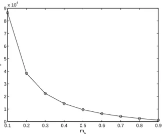
0.1 0.2 0.3 0.4 0.5 0.6 0.7 0.8 0.9 0 1 2 3 4 5 6 7 8 9x 10 4 m_b n

Figure 3.4: The Relationship Between the Expected Value of X (i.e. m_b) and the Required Number of Samples n

where CX(υ) = ln(MX(υ)) denotes the cumulant generating function with the moment

gen-erating function MX(υ) defined as

M_X(υ) = E[eυx] = m_beυ+ 1 − m_b (3.11) The main concern is to obtain a feasible value of n such that Pb,k will approach the expected

value mb (in (3.8)). Considering P

¡¯ ¯1 n P_n i=1Xi− mb ¯ ¯ > 0.04 mb ¢ ≤ 10−3 _{(from (3.9)) as the}

criterion for acquiring the n value, and the relationship between mb and n can be illustrated

as in Fig. 3.4 from the range of m_b = 0.1 to 0.9. It can be observed that the maximum required number of the sample points (n) is close to 105 _{in the m}

b = 0.1 case. Therefore,

the considered time interval ∆T can be computed as ∆T = n · σ = 105_{× (20 × 10}−6_{) = 2}

sec by adopting the DSSS case. Assuming that the maximum size of a packet equals to 1024 bytes, the required transmission time of the packet can be found around 4 ms ∼ 10 ms, which depends on both the channel bit rate and the propagation delay. It can be observed that the selected time interval ∆T = 2 sec is longer enough comparing with the packet transmission time in order to support the convergent theory in (3.8); while it is not too lengthy as being capable to capture the latest channel information. It is also noticed that different values of ∆T can be acquired with the similar procedures for other specifications.

Chapter 4

Analytical Study on the Effects

from Data Rate and Neighbor

Interference

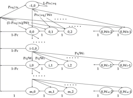
The influence from the data rate and the neighbor interference to the network performance will be investigated in this chapter. Analytical study is performed in order to explore the benefits of the proposed CNAR protocol. There are existing research [25] - [30] establishing the analytical models for the IEEE 802.11 MAC protocol under certain assumptions. An IEEE 802.11 backoff model is proposed in [25] under the saturation state; while the non-saturated model is presented in [26]. Most of the related research are devoted on proposing precise models in order to fully emulate the behavior of IEEE 802.11 MAC mechanism. However, these models are inherently intricate with non-closed form nature. It becomes difficult to conduct further performance analysis by exploiting these existing models, e.g. hard to investigate the relationship between the network performance and the model parameters.

In this chapter, the backoff model of the IEEE 802.11 protocol [26] is extended and in-tegrated with the M/M/1 queuing system [31] for analyzing the network performance. It is noticed that the purpose of this chapter is not to propose a comprehensive analytical MAC model, but to provide a methodology in order to analytically illustrate the effectiveness of

-1,0

0,0 0,1 0,2 0,W -20 0,W -10

0,W -2i 0,W -1i

0,W -m2 0,W -1m i-1,0

i,0 i,1 i,2

m,0 m,1 m,2 1 1 1 1 1 1 1 1 1 1 1 1 1-Pc 1 1-Pc 1-Pc Pc/Wi Pc/Wi Peq|tx 1-Ptx|eq (1-Peq|tx)/W0 Pc/Wi Ptx|eq/ W0

Figure 4.1: The Embedded Markov Chain Model for IEEE 802.11 Backoff Mechanism the proposed CNAR algorithm. For simplicity, (i) only the localized effect is considered in the derivation of the model and (ii) it is assumed that the transmission range of each SN is comparably larger than the distance between the neighbor SNs. The packet delivery ratio will be evaluated under different numbers of the interfering SNs and the data rates acquired form the application layer.

4.1

Analytical Modeling of the IEEE 802.11 Protocol

The embedded Markov chain of the IEEE 802.11 backoff mechanism is shown in Fig. 4.1. The backoff timer at the ith _{stage can be represented as W}

i = 2i · W , where W denotes

the minimum contention window, and i ∈ [0, m] with m representing the maximum backoff stage. The backoff state (s(t), b(t)) (as illustrated in Fig. 4.1) consist of two discrete-time stochastic processes, i.e. s(t) indicates the backoff stage i ∈ [0, m] and b(t) denotes the backoff counter for each SN. It is also noted that the state (-1,0) is introduced on behalf of the empty queue within a SN. In order to facilitate the computation of the transition probability P_t, three associated probabilities are introduced, i.e. (i) P_c: the conditional packet collision probability, (ii) P_tx|eq: the probability of an incoming transmission obtained

after an empty queue in a SN, and (iii) P_eq|tx the probability of an empty queue is observed after a successful transmission or a maximum backoff. The values of these three probabilities will be computed later in this section. Therefore, the transition probabilities, shortly denoted as Pt(i1, k1| i0, k0) , Pt(s(t + 1) = i1, b(t + 1) = k1| s(t) = i0, b(t) = k0), can be obtained as follows:                                                Pt(i, k | i, k + 1) = 1 k ∈ [0, Wi− 2], i ∈ [0, m] Pt(i, k | i − 1, 0) = _WiPc k ∈ [0, Wi− 1], i ∈ [1, m] Pt(−1, 0 | i, 0) = (1 − Pc) · Peq|tx i ∈ [0, m − 1] Pt(−1, 0 | m, 0) = Peq|tx P_t(0, k | i, 0) = (1−Pc)(1−Peq|tx) W0 k ∈ [0, W0− 1], i ∈ [0, m − 1] Pt(0, k | m, 0) = 1−P_Weq|tx₀ k ∈ [0, W0− 1] P_t(0, k | − 1, 0) = P_tx|eq· 1 W0 k ∈ [0, W0− 1] (4.1)

By defining the stationary distribution as Si,k = limt→∞Pt(s(t) = i, b(t) = k) with i ∈ [0, m]

and k ∈ [0, W_i− 1], the state probabilities can be acquired from Fig. 4.1 as S0,k = W_W0− k

0

£

S−1,0· Ptx|eq+ (1 − Peq|tx)Psum

¤ k ∈ [0, Wi− 1] (4.2) Si,k = W_Wi− k i Pc· Si−1,0= Wi− k Wi P i c· S0,0 k ∈ [0, Wi− 1], i ∈ [1, m] (4.3)

S_−1,0 = (1 − P_tx|eq) · S_−1,0+ P_eq|tx· P_sum (4.4) where Psum =

P_m−1

i=0 (1 − Pc) · Si,0+ Sm,0. After the reorganization on (4.2), (4.3), and (4.4),

the state probabilities can be concisely represented as

S−1,0 = P_eq|tx P_tx|eq · Psum (4.5) S_i,k = Wi− k W_i · P i c· S0,0 k ∈ [0, Wi− 1], i ∈ [0, m] (4.6)

As a consequence, the state probability S_0,0 can be determined as S0,0 = Ã _m X i=0 Wi−1_X k=0 Wi− k Wi · P i c+ P_eq|tx P_tx|eq !−1 = µ 1 2 · 1 − (2Pc)m+1 1 − 2P_c W0+ 1 − Pm+1 c 1 − P_c ¸ +Peq|tx P_tx|eq ¶₋₁ (4.7) On the other hand, The probability of any transmission within a SN in a randomly selected time slot (i.e. the conditional transmission probability τ ) can be expressed as

τ = m X i=0 Si,0 = 1 − P m+1 c 1 − Pc S0,0 (4.8)

Assuming that there are α interfering neighbor SNs, the conditional collision probability P_c can therefore be obtained as

Pc= 1 − (1 − τ )α−1 (4.9)

Under the assumption of Poisson traffic with average data arrival rate λ (with unit as packets per second), the conditional probability P_tx|eq is acquired as

P_tx|eq = (1 − e−λσ)(1 − τ )α−1+ (1 − e−λTtx)[1 − (1 − τ )α−1] (4.10) where σ is the slot time length, and Ttx is denoted as the average transmission time as

Ttx = (1 − Pc) · Ts+ Pc· Tc. It is noted that Ts represents the time required for a successful

transmission; while Tc is the time for packet collision, i.e.

T_s = T_{RT S}+ T_{CT S}+ T_ACK + 3 T_{SIF S}+ T_{DIF S}+ T_ϑ+ 4 T_δ (4.11)

Tc = TRT S+ TDIF S+ Tδ (4.12)

where T_δdenotes the propagation delay, and T_ϑis the time required for transmitting the data packet. Moreover, with the consideration of moderate traffic load, the conditional probability

P_eq|tx can be approximated as [29]

P_eq|tx= e−λTsv (4.13)

where the average service time (including the backoff and the transmission states) of a packet is expressed as T_sv = m−1_X i=0 Pi c P_m j=0Pcj (1 − P_c) " T_s+ i T_c+ i X k=0 W_k− 1 2 σ # + P m c P_m j=0Pcj " Ts(1 − Pc) + PcTc+ m Tc+ m X k=0 Wk− 1 2 σ # (4.14) with the average time between the successive backoff timers denoted as σ = σ(1 − τ )α−1 ₊

Ttx·

£

1 − (1 − τ )α−1¤_{. By substituting (4.10) and (4.13) into (4.7), the state probability S}

0,0

becomes a function of the conditional collision probability Pcand the conditional transmission

probability τ . After incorporating (4.7) into (4.8) and (4.9), the values of Pc and τ can

therefore be obtained.

There are three different behaviors that can happen within a SN for handling an outgoing packet, i.e. successful packet transmission, packet collision, and packet withdraw after the maximum retransmission. Therefore, the effective service rate µ_e can be represented as

µe = (1 − Pc) · µs+ Pw· µw+ (Pc− Pw) · µc (4.15)

where the probability for withdrawing a packet is P_w = P_c· S_m,0/(Pm_i=0S_i,0) = [Pm+1

c (1 −

(µ_w), and packet collision (µ_c) are expressed as µs = Ã Ts+ m X i=0 Wi− 1 2 · σ · Pi c P_m j=0Pcj !₋₁ (4.16) µw = µ Tc+Wm₂− 1· σ ¶₋₁ (4.17) µ_c = Ã T_c+ m−1_X i=0 W_i− 1 2 · σ · Pi c P_m−1 j=0 Pcj !₋₁ (4.18) By mapping the system into the M/M/1 queueing model, the complete rate for the successful transmission can be represented as

CR_s= E[U ] · (1 − P_c)µ_s= ρ · (1 − P_c)µ_s (4.19) where the expectation value of the queue utilization (U ) is E[U ] = ρ for the M/M/1 queueing system. It is noted that the parameter ρ corresponds to the traffic intensity and is expressed as ρ = λ/µe. Therefore, the packet delivery ratio can be acquired as

R = CRs

λ = (1 − Pc) · µs

µ_e (4.20)

with µe and µsobtained from (4.15) and (4.16). In the next section, the packet delivery ratio

R will be utilized as the criterion for evaluating the network performance under different data

rates and interfering neighbor SNs.

4.2

Analytical Study on the Network Performance

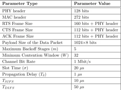
The network performance will be analyzed in this section by employing both the analytical and the simulation results. The performance will be evaluated by considering the packet delivery ratio versus both the data rate and the neighbor interference. Table 4.1 summarizes the parameters adopted from the DSSS system for both the analytical and the simulation results. The packet delivery ratio R computed from (4.20) will be utilized as the analytical results; while the simulation results are conducted via the Network Simulator (ns-2, [21]).

Table 4.1: Analytical and Simulation Parameters Adopted from the DSSS System

Parameter Type Parameter Value

PHY header 128 bits

MAC header 272 bits

RTS Frame Size 160 bits + PHY header CTS Frame Size 112 bits + PHY header ACK Frame Size 112 bits + PHY header Payload Size of the Data Packet 1024×8 bits

Maximum Backoff Stages (m) 5 Minimum Contention Window (W ) 32

Channel Bit Rate 1 Mbit/s

Slot Time (σ) 20 µs

Propagation Delay (Tδ) 1 µs

TSIF S 10 µs

TDIF S 50 µs

In order to illustrate that one transmission pair is interfered by another α pairs of packet delivery, the simulations are performed with (α + 1) pairs of SNs for point-to-point packet delivery within the same transmission range.

Before exploring the performance on the packet delivery ratio R, an important parameter (i.e. the service time Tsv from (4.14)) will be investigated first. Figs. 4.2 and 4.3 show the

comparison of T_sv versus the application layer data rate (λ) and the number of interfering neighbors (α). As shown in both plots with lower data rate and smaller number of interfering neighbors, the value of service time (i.e. Tsv ≈ 0.01 sec) is observed to be similar to the

successful transmission time Ts = 0.0094 sec, which can be calculated from (4.11) via the

data from Table I. The results indicate that there is almost no packet collision under these situations, which make Tsv similar to Ts without the necessity for considering the backoff

time in (4.14). In most of the cases, the service time is perceived to significantly increase from a Critical Point (CP) either the data rate or the number of the interfering neighbors is augmented. The CP corresponds to the location of the channel capacity as C , 1/T_sv, which is defined as the maximum services of the packets per unit time. On the other hand, the total incoming packets per unit time obtained from the interfering neighbor SNs are computed as

2 4 6 8 10 12 14 0.005 0.01 0.015 0.02 0.025 0.03 0.035 0.04 λ (packets/sec) Tsv (sec) α=6 α=9 α=12

Figure 4.2: Service Time (Tsv) vs. Data Rate (λ)

2 4 6 8 10 12 14 16 0.005 0.01 0.015 0.02 0.025 0.03 0.035 α Tsv (sec) λ=5 λ=7.5 λ=10

the cases that the total interfering effect T = λ α is around the same value or larger than the channel capacity C. Due to the system saturation, the service time will be significantly increased since the additional time is required for packet retransmission and collision. This assertion can also be validated by observing the CPs from both of Figs. 4.2 and 4.3. The CP for α = 12 and λ = 7.5 (such that T = λ α = 90) corresponds to the channel capacity calculated as C = 91.07; and the CP for α = 9 and λ = 10 (such that T = 90) corresponds to

C = 91.87. It is noted that C = 1/Tsv, where the average service time Tsv is computed from

(4.14). It can be perceived that both T and C share the similar values in these cases, which validate the existence of the CP where the system saturation occurs.

Fig. 4.4 shows the performance comparison for packet delivery ratio versus the application layer data rates under α = 6, 9, and 12; while Fig. 4.5 illustrates the comparison for packet delivery ratio versus different numbers of interfering neighbors with λ = 5, 7.5, and 10. From both plots, it can be observed that the analytical results is consistent with that acquired from the simulations, which validate the correctness of the derived analytical model. Similar to the observations from Figs. 4.2 and 4.3, the performance degradation is perceived from the location of the CP either the data rate or the number of the interfering neighbors is increased. As T < C, comparably higher packet delivery ratio R can be achieved since most of the packets can be successfully delivered. On the other hand, as T reaches or exceeds the channel capacity C, some of the packets will not be transmitted due to the system saturation that causes the rapid decreases in the packet delivery ratio.

The above observations support the effectiveness of the proposed CNAR protocol with efficient usage of the system resources. The CNAR algorithm is designed to cognitively select the routing path, which inherently possesses smaller probability for packet collision. The total interfering effect from the neighbor SNs can be diminished such that the SNs within the route will not reach their channel capacities C. The proposed CNAR scheme can therefore conduct data delivery under better channel quality without wasting the limited system resources. Moreover, the performance study in this chapter only consider the localized effect for packet transmission with infinite data queue in each SN. The system saturation problem can become

more severe by considering both (i) the hidden terminal problem and (ii) the finite queueing effect under the multi-hop data delivery. It is noted that the hidden terminal problem will further cause the interference from the tow-hop away neighbor SNs. The substantial benefits of using the proposed CNAR algorithm can become obvious under such realistic multi-hop environments. In the next chapter, the CNAR scheme will be compared with other existing protocols via simulations which emulate the environments of the WSNs.

2 4 6 8 10 12 14 0.75 0.8 0.85 0.9 0.95 1 λ (packets/sec)

Packet Delivery Ratio (%)

simulation(α=6) simulation(α=9) simulation(α=12) α=6 α=9 α=12

Figure 4.4: Packet Delivery Ratio vs. Data Rate λ (Solid Lines: Analytical Results; Dashed Lines: Simulation Results)

2 4 6 8 10 12 14 16 0.75 0.8 0.85 0.9 0.95 1 α

Packet Delivery Ratio (%)

simulation(λ=5) simulation(λ=7.5) simulation(λ=10) λ=5 λ=7.5 λ=10

Figure 4.5: Packet Delivery Ratio vs. Number of Interfering Neighbors α (Solid Lines: Ana-lytical Results; Dashed Lines: Simulation Results)

Chapter 5

Performance Comparison and

Evaluation

The Network Simulator (ns-2, [21]) is utilized to implement the proposed CNAR algorithm and to compare with the other existing routing protocols, i.e. the AODV and the LBAR protocols. The following three criterions are utilized as the performance metrics:

1. The Packet Delivery Ratio (%): The ratio of the number of the received data packets to the number of the total data packets sent by the sources.

2. The Average End-to-End Delay (sec): The average time elapsed for delivering a data packet within a successful transmission.

3. The Power Consumption from the Control Overhead (Watt): The total power consumed by sending the required control packets.

The following two scenarios are conducted in the simulations for performance comparison:

5.1

The Grid Topology

The grid topology as shown in Fig. 3.1 is utilized for the first performance comparison. Table 5.1 illustrates the parameters that are adopted for the grid topology. It is noted that different

Table 5.1: Simulation Parameters for the Grid Topology

Parameter Type Parameter Value Transmission Range 10 m

Propagation Model TwoRayGround Transmission Power 25 dBm

Traffic Types Constant Bit Rate (CBR)

MAC IEEE 802.11 DCF

Data Rate R1, R2 : 5 packets/sec

Size of Data Packet R1, R2 : 512 Bytes

R3 : 1024 Bytes

Transmission Time R1 : 400 - 1000 sec

R2, R3 : 0 - 600 sec

Total Simulation Time 1200 sec

data rates, data sizes, and starting time instants for data transmissions are utilized within the three different routes, R₁, R₂, and R₃.

Figs. 5.1 to 5.3 show the performance comparisons between the three schemes under different data rates (packets/sec) along the route R3 (i.e. υ3 goes from 5 to 35 packets/sec).

It is noticed that R2 and R3 initiate their packet transmission earlier than R1 as denoted in

Table 5.1. As can be seen from Figs. 5.1 and 5.2 that the performance of the AODV protocol is severely degraded as the data rate of R3 is increased, i.e. with decreased packet delivery

ratio and increased average end-to-end delay. The reason is primarily attributed to that the total interfering effect T reaches the channel capacity C around the data rate of R3 = 15

packets/sec. The AODV protocol selects p_1,1 of R1 for packet forwarding, which results in

significant waste of channel resources due to the packet collision. On the other hand, the LBAR scheme conducts packet transmission using the path p_1,3 of R₁, which is based on the path cost as defined in (2.1). Reasonable routing performance can be observed using the LBAR scheme as shown in Figs. 5.1 and 5.2. However, the LBAR protocol causes substantial power consumption on sending the control packets comparing with the CNAR and the AODV schemes (as in Fig. 5.3). Due to its excessive usage of the hello packets, around three orders more power consumption can be observed by adopting the LBAR scheme.

algorithms, e.g. around 5% and 40% more on the packet delivery ratio comparing with the LBAR and the AODV schemes (under data rate = 30 packets/sec). Due to the severe channel congestion around the path p_1,1, the CNAR protocol utilizes p_1,3 of R1 under the case of

the lower date rate in R3 and adopts p1,2 of R1 at the higher data rate of R3 for packet

forwarding between t = 400 to 600 sec. It is noted that the CNAR protocol outperforms the LBAR scheme by selecting p_1,2of R1under the circumstance with higher data rate of R3. The

cognitive path-switching mechanism within the CNAR scheme changes the path back to p_1,1 after t > 600 sec, i.e. after the channel quality is improved due to the termination of R2 and

R₃. With the adopting of moderate amount of control packets (which are excessively utilized in the LBAR scheme), the CNAR protocol can cognitively exploit the channel resources more effectively using its inherent MAC capability, i.e. the NAV vectors obtained from both the RTS and the CTS packets.

5.2

The Random Topology

The random topology is also utilized to evaluate the proposed CNAR protocol, with the corresponding simulation parameters are shown in Table 5.2. It is noted that the starting time for packet transmission of each source node is randomly selected between 0 and 1500 seconds; while the data size is chosen between 512 and 1024 bytes.

Figs. 5.4 - Fig. 5.9 show the performance comparison of these three protocols under (i) different numbers of source nodes (as in Figs. 5.4 to 5.6 with average1 _{data rate = 10}

packets/sec); and (ii) different average data rates (as in Figs. 5.7 to 5.9 with the number of source = 20). It is observed that the proposed CNAR protocol outperforms the other two protocols with higher packet delivery radio and lower end-to-end delay. There are around 5% and 10% more in the packet delivery ratio; 0.5 and 2 seconds less in the end-to-end delay comparing with the LBAR and the AODV methods (under the number of source node = 30 as in Figs. 5.4 and 5.5). Due to the route-averaging effect, the severe system saturation incurred by the AODV protocol (as in Figs. 5.1 and 5.2) is not noticeable in the random

Table 5.2: Simulation Parameters for the Random Topology

Parameter Type Parameter Value Simulation Area 50 × 25 m2

Transmission Range 10 m

Propagation Model TwoRayGround Transmission Power 25 dBm

Number of Nodes 60

Traffic Types Constant Bit Rate (CBR)

MAC IEEE 802.11 DCF

Maximum Transmission Time 600 sec of Each Source

Total Simulation Time 1700 sec

topology. Nevertheless, a comparably larger amount of routes selected by the proposed CNAR algorithm will not reach their channel capacities, which make the scheme possesses better routing performance in average.

Comparing with the AODV protocol, the CNAR algorithm generates a slightly higher power consumption from the control packet overhead due to the additional usage of the RREQ packets. However, the CNAR protocol consumes significantly less energy in the control overhead than that from the LBAR algorithm, e.g. around 1.5 order less in power consumption as in Fig. 5.9 (under different average data rates). The merits of using the CNAR algorithm can be observed from these simulation results. Even with the existence of channel congestion, the proposed CNAR protocol can offer better routing performance by cognitively adjusting the utilization of the channel resources.

0 5 10 15 20 25 30 35 0.55 0.6 0.65 0.7 0.75 0.8 0.85 0.9 0.95 1 Data Rate of R₃

Packet Delivery Ratio

CNAR LBAR AODV

Figure 5.1: Simulation Result of the Grid Topology : Packet Delivery Ratio vs. Data Rate of

R3 0 5 10 15 20 25 30 35 0 0.1 0.2 0.3 0.4 0.5 0.6 0.7 0.8 0.9 Data Rate of R₃ End−to−End Delay CNAR LBAR AODV

Figure 5.2: Simulation Result of the Grid Topology : Average End-to-End Delay vs. Data Rate of R3

0 5 10 15 20 25 30 35 1 1.5 2 2.5 3 3.5 4 Data Rate of R₃

Power Consumption in Log Scale

CNAR LBAR AODV

Figure 5.3: Simulation Result of the Grid Topology : Power Consumption from Control Overhead vs. Data Rate of R3

0 5 10 15 20 25 30 0.55 0.6 0.65 0.7 0.75 0.8 0.85 0.9 0.95 1 Number of Sources

Packet Delivery Ratio

CNAR LBAR AODV

Figure 5.4: Simulation Result of Random Topology : Packet Delivery Ratio vs. Number of Sources

0 5 10 15 20 25 30 0 1 2 3 4 5 6 Number of Sources End−to−End Delay CNAR LBAR AODV

Figure 5.5: Simulation Result of Random Topology : Average End-to-End Delay vs. Number of Sources 0 5 10 15 20 25 30 2 2.5 3 3.5 4 4.5 Number of Sources

Power Consumption in Log Scale

CNAR LBAR AODV

Figure 5.6: Simulation Result of Random Topology : Power Consumption from Control Overhead vs. Number of Source