A design approach to the multi-objective facility layout problem

(1)

On: 28 April 2014, At: 03:39 Publisher: Taylor & Francis

Informa Ltd Registered in England and Wales Registered Number: 1072954 Registered office: Mortimer House, 37-41 Mortimer Street, London W1T 3JH, UK

International Journal of

Production Research

Publication details, including instructions for authors and subscription information: http://www.tandfonline.com/loi/tprs20

A design approach to the

multi-objective facility

layout problem

C.-W. Chen

Published online: 15 Nov 2010.

To cite this article: C.-W. Chen (1999) A design approach to the multi-objective facility layout problem, International Journal of Production Research, 37:5, 1175-1196, DOI: 10.1080/002075499191463

To link to this article: http://dx.doi.org/10.1080/002075499191463

PLEASE SCROLL DOWN FOR ARTICLE

Taylor & Francis makes every effort to ensure the accuracy of all the information (the “Content”) contained in the publications on our platform. However, Taylor & Francis, our agents, and our licensors make no representations or warranties whatsoever as to the accuracy, completeness, or suitability for any purpose of the Content. Any opinions and views expressed in this publication are the opinions and views of the authors, and are not the views of or endorsed by Taylor & Francis. The accuracy of the Content should not be relied upon and should be independently verified with primary sources of information. Taylor and Francis shall not be liable for any losses, actions, claims, proceedings, demands, costs, expenses, damages, and other liabilities whatsoever or howsoever caused arising directly or indirectly in

connection with, in relation to or arising out of the use of the Content. This article may be used for research, teaching, and private study purposes. Any substantial or systematic reproduction, redistribution,

(2)

and use can be found at http://www.tandfonline.com/page/terms-and-conditions

(3)

A design approach to the multi-objective facility layout problem C.-W. CHEN² _{and D. Y. SHA}² _*

A new multi-objective heuristic algorithm for resolving the facility layout problem is presented in this paper. It incorporates qualitative and quantitative objectives and resolves the problem of inconsistent scales and di erent measurement units. We consider suboptimal solutions since optimal methods are computationally unfeasible to large layout problems. In this paper, we develop the dominant index (DI)and incorporate it in our heuristic algorithm to guarantee the quality of proposed solutions. Moreover, a new measure of solution quality, dominant probability (Dp), is o ered to determine the probability that one layout is better than the others. Computational results show that our proposed heuristic algor-ithm is an e cient method for obtaining good-quality solutions.

1. Introduction

The facility layout problem deals with ® nding the most e ective physical arrange-ment of facilities, personnel, and any resources required to facilitate the production of goods or services. It has attracted the attention of many researchers because of its practical utility and interdisciplinary importance. Historically, two basic approaches have most commonly been used to generate desirable layouts: a qualitative one and a quantitative one. These approaches are usually used one at a time when solving a facility layout problem.

With qualitative approaches, layout designers provide subjective evaluations of desired closeness between departments. Then, overall subjective closeness ratings between various departments are maximized. These subjective closeness ratings can be used: A (absolutely necessary

)

, E (essentially important

)

, I (important

)

, O (ordinary

)

, U (unimportant

)

and X (undesirable

)

, to indicate the respective degrees of necessity that two given departments be located close together. Layout designers may then assign numerical values to the ratings such that they have the ranking A > E > I > O > U > X. Seehof and Evans (1967

)

, Lee and More (1967

)

, Muther and McPherson (1970

)

and Muther (1973

)

have developed algorithms based on qualitative criteria to obtain ® nal layouts. These di erent qualitative approaches are distinguished primarily by the scoring methods used for the closeness ratings. For example, the numerical values used by Sule (1994

)

and Harmonosky and Tothero (1992

)

for these ratings are A 4, E 3, I 2, O 1, U 0 and X 1. Another example, the ALDEP procedure presented by Seehof and Evans (1967

)

used the numerical values: A 64, E 16, I 4, O 1, U 0 and

X 1024.

Quantitative approaches involve primarily the minimization of material handling costs between various departments. The quadratic assignment problem (QAP

)

for-0020± 7543/99 $12.00Ñ 1999 Taylor & Francis Ltd. Revision received July 1997.

² Department of Industrial Engineering and Management, National Chiao Tung University, 1001 Ta Hsueh Road, Hsinchu, Taiwan 30010, Republic of China.

*To whom correspondence should be addressed.

(4)

mulation for assigning n facilities to n mutually exclusive locations is the most typical model used. Gilmore (1962

)

, Lawler (1963

)

and Gavett and Plyter (1966

)

have o ered exact solution procedures using branch-and-bound techniques. However, the QAP formulation belongs to the class of NP-complete problems (Garey and Johnson 1979

)

, and no known method can arrive at an optimal solution in a reason-able time when 15 or more facilities are considered. Consequently, many heuristic algorithms have been developed for achieving a trade-o between computation time and the e ciency of the ® nal solution (Kusiak and Heragu 1987

)

and our proposed approach is also a heuristic one.

Many researchers have questioned the appropriateness of selecting a single-criterion objective to solve the facility layout problem because qualitative and quan-titative approaches each have advantages and disadvantages. The major limitations on quantitative approaches are that they consider only relationships that can be quanti® ed and to not consider any qualitative factors. The shortcoming of qualita-tive approaches is their strong assumption that all qualitaqualita-tive factors can be aggre-gated into one criterion. In real life, the facility layout problem must consider quantitative and qualitative criteria and this falls into the category of the multi-objective facility layout (MOFL

)

problem.

The primary purpose in solving the MOFL problem is to generate e cient alter-natives that can then be presented to the decision maker for his or her selection. Malakooti (1989

)

classi® ed three types of methods for solving the MOFL problem: (a

)

generate the set of e cient layout alternatives and then present it to the decision maker; (b

)

assess the decision maker’s preferences ® rst, and then generate the best layout alternative, and (c

)

use an interactive method to ® nd the best layout alter-native. Our proposed approach in this paper falls into the category of the type (a

)

methods in terms of generating good-quality solutions using an e ective heuristic algorithm. With respect to type (a

)

methods, Rosenblatt (1979

)

, Dutta and Sahu (1982

)

, Fortenberry and Cox (1985

)

, Waghodekar and Sahu (1986

)

, Urban (1987, 1989

)

and Houshyar (1991

)

, Harmonosky and Tothero (1992

)

all developed QAP formulations by specifying di erent objective weights to generate the best layout. However, there are two inadequacies in these approaches:

(1

)

all factors may not be represented on the same scale; (2

)

measurement units used for objectives may be incomparable.

In this paper we present an e ective approach that overcomes the above-men-tioned inadequacies by reasonably normalizing all objectives of the MOFL problem, and handling qualitative and quantitative information in similar fashion. Because existing optimization methods are computationally ine cient when large numbers of facilities are involved, heuristic methods are more appropriate for generating e ec-tive layouts. Kusiak and Heragu (1987

)

have suggested a measure for assessing the quality of solutions for the single-objective facility layout problem. However, eval-uating various solutions to the MOFL problem is di cult because of the lack of a suitable measure for e ectiveness with respect to multiple objectives. In this paper, a new measure for the MOFL problem, dominant probability (Dp

)

, is presented that determines the probability that one layout is better than the others. Moreover, we develop the dominant index (DI

)

and combine it with our heuristic algorithm to guarantee the quality of solutions.

In section 2 we give an overview of MOFL models; our heuristic approach is presented in section 3. The heuristic algorithm for the proposed approach is

(5)

sented in section 4, and a numerical example is given in section 5. In section 6, the e ectiveness of the proposed approach is demonstrated by solving some problems cited in the literature. Section 7 concludes the paper.

2. Review of past approaches

The QAP formulation of the MOFL problem is shown in equations (1

)

to (4

)

Minimize Z n i 1 n j 1 n k 1 n l 1 aijklXijXkl 1 subject to n i 1 Xij 1 j 1

,

. . .

,

n 2 n j 1 Xij 1 i 1

,

. . .

,

n 3 Xij 0

,

1 i

,

j 1

,

. . .

,

n

,

4 where Xij

1 if facility i is assigned to location j

,

0 otherwise,

Aijkl the cost of locating facility i at location j and facility k at location l.

Aijkl in equation (1

)

is a cost variable representing the combination of quantitative

and qualitative measures in MOFL models. Equation (2

)

ensures that each location contains only one facility. Equation (3

)

ensures that each facility is assigned to only one location. We divided these models presented in previous studies into four cate-gories:

(1

)

Rosenblatt (1979

)

and Dutta and Sahu (1982

)

de® ned the cost term as: Aijkl WcCijkl WRRijkl

,

5

where Cijklis the total material handling cost, Rijklis the total closeness rating

score, and Wc and WR are weights assigned to the total material handling cost and to the total rating score.

(2

)

Foretenberry and Cox (1985

)

de® ned the cost term as:

Aijkl fik djl rik

,

6

where fik is the work ¯ ow between two facilities, djl is the distance between

two locations and rikis the closeness rating desirability of the two facilities.

(3

)

Urban (1987, 1989

)

Aijkl djl fik C rik

,

7

where C is a constant weight that determines the importance of the closeness rating to the work ¯ ow.

(4

)

Khare et al. (1988b

)

Aijkl W1 rik djl W2 fik djl

,

8

(6)

where W1and W2are weights assigned to the work ¯ ow and to the closeness rating.

The listed models are similar in nature, and vary only in stating the relationship between the cost term Aijkl and the quantitative and qualitative measures. Although

these models have been applied to the MOFL problem, they all have two inadequa-cies.

(1

)

All factors may not be represented on the same scale: for example, values for work ¯ ow may range from zero to a tremendous amount, while closeness rating values may range from 1 to 4. As a result, the closeness ratings would be dominated by work ¯ ow and have little impact on the ® nal layout (Harmonosky and Tothero 1992

)

.

(2

)

Measurement units used for objectives may be incomparable: the closeness rating represents an order preference indicating the necessity that given facil-ities be located close together. The total closeness rating score is only an ordinal value; on the other hand, the material ¯ ow handling is measured according to cost. Combining these two values with di erent measurement units in an algebraic operation is unsuitable.

For the reasons cited above, Harmonosky and Tothero (1992

)

suggested an approach that normalizes all factors, before combining them. To normalize a factor, each relationship value is divided by the sum of all relationship values for that factor, as shown in equation (9

)

:

Tikf nSikf

i nkSikf

,

9

where

Sikf is the relationship value between departments i and k for factor f , and

Tikf is the normalized relationship value between departments i and k for factor f .

Next, all values are multiplied by weights representing the relative importance of each factor f . Then, the sum of all values for each pair of departments is calculated. The resulting objective function is shown in equation (10

)

:

Minimize Z n i 1 n j 1 n k 1 n l 1 t f 1

a

f TikfdjlXijXkl

,

10

where

a

f is the weight for factor f .

Harmonosky and Tothero (1992

)

proposed a methodology for normalizing all factors into comparable units on the same scale. However, the scaling problem remains unresolved. Note ® rst that values for work ¯ ow may range from zero to a very large positive value, while closeness rating values may range from a negative value to a positive value. After using equation (9

)

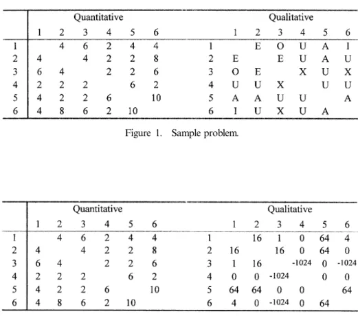
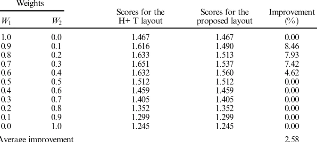
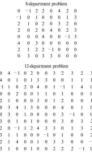
, most normalized relationship values of the larger scaling factor are lower than those of the smaller scaling factor. As a result, the larger scaling factor would have very little e ect on the ® nal layout. Second, di erent scoring values for the closeness ratings may cause some inadequacies. For example, we take the same sample problem from Harmonosky and Tothero (1992

)

and show it in ® gure 1. Then we take the values used by ALDEP (Seehof and Evans 1967

)

to quantify the qualitative factor, and the

(7)

resulting qualitative matrix is shown in ® gure 2, along with the quantitative matrix. The result of normalization using equation (9

)

for this problem is shown in ® gure 3. In this ® gure, value A in the qualitative matrix of ® gure 1 is converted into the largest negative value and X is converted into the largest positive value. In this case, it is inadequate to use the resulting qualitative matrix to generate solutions to this prob-lem.

In order to resolve the scaling and measurement problems simultaneously, we developed an e ective alternative approach to normalize reasonably all objectives before combining them.

3. Development of a new multi-objective approa ch

Wallace et al. (1976

)

presented a method for computing the variance of the cost distribution associated with the facility layout problem using only the basic data on ¯ ow, distance and problem size. Subsequently, re® nements were given in Sahu and Sahu (1979

)

, and Dutta and Sahu (1981

)

. However, they considered only the forward movement of materials. Khare et al. (1988a

)

extended these methods to consider both forward and backward movement of materials, and showed that the layout cost distribution closely approximates a normal distribution. The general expression for variance proposed by Khare et al. (1988a

)

is shown in equation (11

)

. The mean of all feasible layout costs can also be computed (Nugent et al. 1968

)

:

Figure 1. Sample problem.

Figure 2. Quantitative and qualitative factors expressed numerically.

(8)

Vc _{n n 1}2 n i 1 n j 1 f2 i

,

j n 1 i 1 n j i 1 d2 i

,

j n2 n 12M2fMd2 4 n n 1 n 2 PnfPnd 16QnfQnd n n 1 n 2 n 3 4PnfPnd n n 1 n 2 4 n n 1 n 1 i 1 n j i 1 f i

,

j f j

,

i n 1 i 1 n j i 1 d2 _i

,

_j 16QnfQnd n n 1 n 2 n 3

,

11 where

Vc is the cost distribution variance, f i

,

j is a ¯ ow matrix element, d i

,

j is a distance matrix element,

Mf is the ¯ ow matrix mean, Md is the distance matrix mean,

Pnf

,

Pnf

,

Qnf

,

Qnf are the products of ¯ ow matrix elements,

Pnd

,

Pnd

,

Qnd

,

Qnd are the products of distance matrix elements. Figure 3. Normalized relationships.

(9)

In order to achieve normalization, we subtract the mean of the layout cost distri-bution from each objective value and divide the result by the standard deviation of all feasible layout costs, as shown in equation (12

)

:

Hm n i nj nk nl Sijklm Mm Vm1/2

,

12 where

Sijklm is the objective value of locating facility i at location j and facility k at

location l for objective m (for m 1

,

. . .

,

t ,

Mm is the mean value of the layout cost distribution for objective m,

Vm is the variance of the layout cost distribution for objective m, and

Hm is the normalized value for objective m.

In this paper, we consider only those objectives with distance-weighted attributes such as ¯ ow and closeness rating. Therefore, we propose this approach for solving the MOFL problem which is based on minimization of distance-weighted objectives, namely minimization of total ¯ ow cost (TFC

)

and minimization of total numerical rating (TNR

)

. The TNR presented by Khare et al. (1988b

)

is given as:

TNR

i j rij dij. 13

Hence, all distance-weighted objective functions in this paper possess the cost variance shown in equation (11

)

and can be characterized as a normal distribution. Using equation (12

)

, we reasonably normalize all objectives, and resolve both the di erent scale and measurement unit problems. The values obtained are then multi-plied by weights (Wm

)

representing the relative importance of each objective. In our

proposed model, the Aijkl in equation (1

)

is represented by equation (14

)

, and the

resulting objective function is shown in equation (15

)

. To simplify the following discussion, we call the objective function, Z, the facility layout score (FLS

)

:

Aijkl t m 1 WmHm

,

14 FLS Z n i n j n k n l t m WmHmXijXkl. 15

Since the layout cost distribution closely approximates a normal distribution (Khare et al. 1988a

)

, the variable Hm is approximately a (standard

)

normal

distri-bution with mean zero and variance 1. Therefore, the variable, FLS, is approxi-mately normally distributed with mean zero and variance Wm2.

In order to guarantee the quality of solutions, we develop a criterion called the dominant index (DI

)

, as shown in equation (16

)

:

DI Za m Wm2 1/2

,

16 where

a

the tolerance probability that the ® nal layout can be dominated (for 0 <

a

< 1

)

, and

Za the standard normal value leaving an area of

a

to the left.

(10)

Using the DI, we develop a heuristic algorithm for obtaining good-quality sol-utions. These solutions are guaranteed to be better than other solutions with a probability of at least 1

a

. We call the fraction 1

a

the dominance con® dence coe cient. Moreover, we present a new measure, dominant probability (Dp

)

, for determining the probability that one solution is better than the others. It is given by:

Dp 1 P Z FLS

W2

m 1/2 .

17

4. Proposed heuristic algorithm

Once these objectives have been reasonably normalized and composed, the MOFL problem can be solved as a single-objective problem. A heuristic algorithm based on the DI is used to generate an e ective layout. Our algorithm is a multi-pass pairwise exchange similar to those presented by Dutta and Sahu (1982

)

and Fortenberry and Cox (1985

)

. This proposed heuristic algorithm is detailed below. Step 0. Read the input data (¯ ow matrix, size of problem n, relationship matrix,

decision weights, a random initial layout, the dominance con® dence coe -cient 1

a

)

.

Step 1. Compute the mean and variance for each objective, the dominant index (DI

)

, and the facility layout score (FLS

)

.

Step 2. Set I 1 and J 2. Step 3. Exchange facility I and J. Step 4. Compute a new FLS.

Step 5. If the new FLS is less than the previous FLS, then go to step 6; otherwise, go to step 7.

Step 6. Set the previous FLS to the new FLS, record the new layout, and go to step 8.

Step 7. Exchange facilities I and J.

Step 8. If J n, go to step 9; otherwise, go to step 10. Step 9. If I n 1, go to step 12; otherwise, go to step 11. Step 10. Set J J 1. Go to step 3.

Step 11. Set I I 1 and J I 1; go to step 3.

Step 12. If FLS has been reduced, go to step 2; otherwise, go to step 13. Step 13. If FLS is less than DI, go to step 15; otherwise, go to step 14. Step 14. Read new input data and compute FLS, go to step 2.

Step 15. Output the best layout, FLS, and the dominant probability Dp. Step 16. Stop.

5. Numerical example

Consider the following plant with 12 departments. These departments will be con® gured in the following 3 4 rectangle. Distance between department locations

(11)

is rectilinear and the width of each location is one unit. The values of work ¯ ow and closeness rating between departments are given in ® gures 4 and 5.

The dominance con® dence coe cient 1

a

is set equal to 0.999, and the weight for total material handling cost (W1

)

is set to 0.5. According to equation (16

)

, we get DI 2.1850. After the proposed procedure, we get a solution with a facility layout score of FLS 3.2782, which is better than DI.

Figure 4. Work ¯ ow matrix.

Figure 5. Closeness rating matrix.

(12)

The dominant probability of this solution is given below: Dp 1 P Z FLS W2 m 1/2 1 P Z 3.2782 0.52 ₀_.₅2 1/2 1 P Z 4.6361 0.999 998.

Since the dominant probability is extremely large in this example, the layout planner can consider accepting the solution.

6. Performance evaluation

The proposed method is evaluated using two standard performance criteria. One is computation time, and the other is the quality of solution. We make a comparison with Harmonosky and Tothero’s procedure (1992

)

using the two test problems in their paper. Further comparisons are made with eight test problems (Nugent et al. 1968

)

solved using other heuristic methods. These comparisons show that our pro-posed method provides acceptable suboptimal solutions in reasonable amounts of computing time. Our proposed algorithm was programmed in the FORTRAN lan-guage and run on a DEC VAX-8650 computer.

6.1. Comparison with Harmonosky and Tothero’s procedure

Harmonosky and Tothero (1992

)

have shown the superiority of their procedure over previous algorithms presented by Rosenblatt (1979

)

, Dutta and Sahu (1982

)

, Fortenberry and Cox (1985

)

and Urban (1987

)

. Therefore, our comparison was made with the results obtained by Harmonosky and Tothero (1992

)

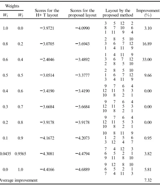
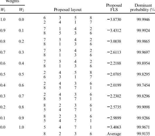
. All layouts for each weight combination generated by our approach were listed and scores were compared. These results are shown in tables 1± 4. Tables 1 and 2 summarize the results for the eight-department problem. Table 1 presents results based on our scoring system, and table 2 is based on Harmonosky and Tothero’s scoring system. Tables 3 and 4 summarize the results for the 12-department problem. All tables show that our proposed procedure is superior to Harmonosky and Tothero’s procedure. 6.2. Test problems

The non-symmetric ¯ ow matrices for the problems of sizes 8, 12, 15 and 20 were taken directly from Khare et al. (1988a

)

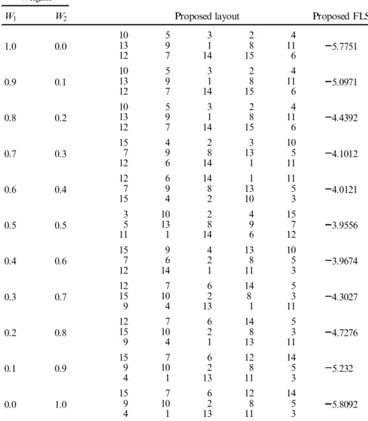
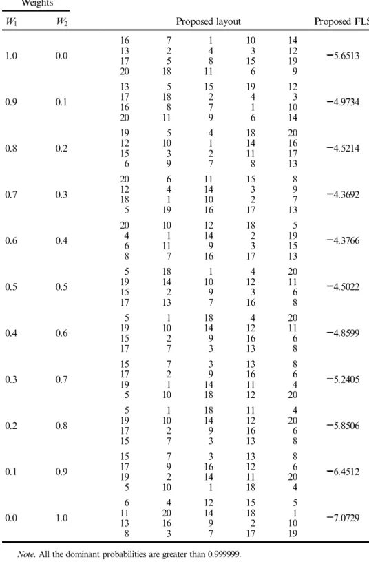
. The corresponding closeness rating matrices for these problems, which were generated by a random number generator are shown in the Appendix. We ran our proposed method using ® ve random initial layouts for each test problem with given weight combinations. We show the best solution for each case in tables 5± 8. According to the dominant probability shown in these tables, our method is capable of obtaining good-quality solutions.

6.3. Computational e ort

To test computational e ort, we generated eight random instances of 10-, 12-, 15-, 20-, 25-, 30-, 36- and 40-facility problems. For each problem size, 100 problems were randomly generated in which work ¯ ow values were taken from a discrete uniform distribution with range [0, 500] and closeness rating values generated at

(13)

Weights

W1 W2

Scores for the

H+ T² layout proposed layoutScores for the proposed methodLayout by the Improvement(%)

1.0 0.0 4.4235 4.4235 ₁2 7₅ 6₈ 4₃ 0.00 0.9 0.1 3.1377 4.1631 ₁2 7₅ 6₈ 4₃ 24.63 0.8 0.2 2.9408 3.9028 ₁2 7₅ 6₈ 4₃ 24.65 0.7 0.3 2.7483 3.6425 ₁2 7₅ 6₈ 4₃ 24.67 0.6 0.4 2.6124 3.3822 ₁2 7₅ 6₈ 4₃ 22.76 0.5 0.5 3.1941 3.1941 ₈6 7₅ 2₁ 4₃ 0.00 0.4 0.6 3.4654 3.4654 ₈6 7₅ 2₁ 4₃ 0.00 0.3 0.7 3.7368 3.7368 ₆8 5₇ 1₂ 3₄ 0.00 0.2 0.8 4.0082 4.0082 ₆8 5₇ 1₂ 3₄ 0.00 0.1 0.9 4.2795 4.2795 ₆8 5₇ 1₂ 3₄ 0.00 0.0 1.0 4.5508 4.5508 ₆8 5₇ 1₂ 3₄ 0.00 Average improvement 9.67

² _{H+ T is a symbol representing Harmonosky and Tothero.}

Table 1. Comparison procedure for the eight-department problem using our scoring system.

Weights

W1 W2

Scores for the

H+ T layout proposed layoutScores for the Improvement(%)

1.0 0.0 1.467 1.467 0.00 0.9 0.1 1.616 1.490 8.46 0.8 0.2 1.633 1.513 7.93 0.7 0.3 1.651 1.537 7.42 0.6 0.4 1.632 1.560 4.62 0.5 0.5 1.512 1.512 0.00 0.4 0.6 1.459 1.459 0.00 0.3 0.7 1.405 1.405 0.00 0.2 0.8 1.352 1.352 0.00 0.1 0.9 1.299 1.299 0.00 0.0 1.0 1.245 1.245 0.00 Average improvement 2.58

Table 2. Comparison procedure for the eight-department problem using H+ T’s scoring system.

(14)

random. Each problem was run individually with an initially random layout. The results shown in table 9 are the average results obtained for the 100 problems of each problem size.

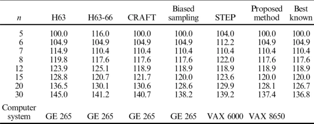
Further proving the e ectiveness of our proposed algorithm, another important comparison was made with other published heuristic approaches to the eight com-monly used test problems proposed in Nugent et al. (1968

)

. For the eight single-objective problems, our solutions were obtained by setting the value of the qualita-tive weight equal to 0. Comparisons were made in terms of the quality of the sol-utions obtained and the computation time required. With respect to the solution quality, Kusiak and Heragu (1987

)

took it as (OV 100

)

/LB, where OV is the objective value and LB is the lower bound as given by Nugent et al. (1968

)

. Thus, the lower the value of the solution quality measure, the better the solution.

Weights

W1 W2

Scores for the

H+ T layout proposed layoutScores for the proposed methodLayout by the Improvement(%)

1.0 0.0 3.9721 4.0990 38 5 127 10 26 3.10 1 11 9 4 0.8 0.2 3.0705 3.6943 23 86 5 107 12 16.89 1 4 11 9 0.6 0.4 2.4046 3.4892 13 4 116 7 129 33.00 2 8 5 10 0.5 0.5 3.0514 3.3777 21 86 5 107 12 9.66 3 4 11 9 0.4 0.6 3.4190 3.4190 12 119 7 65 43 0.00 10 8 2 1 0.3 0.7 3.6684 3.6684 12 119 7 65 43 0.00 10 8 2 1 0.2 0.8 3.9178 3.9178 12 119 7 65 43 0.00 10 8 2 1 0.1 0.9 4.1672 4.2073 101 8 112 5 96 0.95 3 12 4 7 0.0435 0.9565 4.3081 4.4794 76 4 125 2 31 3.82 9 11 8 10 0.0 1.0 4.4166 4.6889 9 126 5 8 102 1 5.81 7 4 11 3 Average improvement 7.32

Table 3. Comparison procedure for the 12-department problem using our scoring system.

(15)

Weights

W1 W2

Scores for the

H+ T layout proposed layoutScores for the Improvement(%)

1.0 0.0 1.991 1.979 0.61 0.8 0.2 2.019 1.967 2.64 0.6 0.4 2.036 1.936 5.17 0.5 0.5 1.916 1.907 0.47 0.4 0.6 1.818 1.818 0.00 0.3 0.7 1.759 1.759 0.00 0.2 0.8 1.701 1.701 0.00 0.1 0.9 1.643 1.619 1.48 0.0435 0.9565 1.610 1.573 2.35 0.0 1.0 1.585 1.538 3.06 Average improvement 1.58

Table 4. Comparison procedure for the 12-department problem using H+ T’s scoring system.

Weights W1 W2 Proposed layout Proposed FLS probability (%Dominant ) 1.0 0.0 6₂ 3₄ 5₁ 8₇ 3.8730 99.9946 0.9 0.1 7₈ 1₅ 4₃ 2₆ 3.4312 99.9924 0.8 0.2 7₈ 5₁ 4₃ 2₆ 3.0038 99.9865 0.7 0.3 7₈ 5₁ 4₃ 2₆ 2.6113 99.9697 0.6 0.4 7₈ 5₁ 4₃ 2₆ 2.2188 99.8954 0.5 0.5 2₆ 4₃ 5₁ 8₇ 2.0705 99.8295 0.4 0.6 2₈ 4₅ 3₇ 6₁ 2.0199 99.7454 0.3 0.7 2₈ 4₅ 3₇ 6₁ 2.2302 99.8296 0.2 0.8 8₅ 2₄ 3₇ 6₁ 2.5735 99.9098 0.1 0.9 8₅ 2₄ 3₇ 6₁ 2.9899 99.9286 0.0 1.0 5 4 7 1 3.4063 99.9671 8 2 3 6 Average 99.9135

Table 5. Problem size n 8 (area limited to two rows and four columns).

(16)

We ran our proposed method with 100 random initial layouts for each test problem. The comparison results are shown in tables 10 and 11. Table 10 gives a comparison of the quality of the best solutions obtained with these heuristic methods, and table 11 gives a comparison of the average solution quality obtained with these heuristic methods. Tables 10 and 11 show that our proposed solutions are better than those provided by other heuristic methods, or are at least as good. As mentioned by Kusiak and Heragu (1987

)

, the computation time provided in table 11 cannot be directly used for comparison because the computation time for each of the

Weights W1 W2 Proposed layout Proposed FLS probability (%Dominant ) 1.0 0.0 76 1011 31 58 4.2233 99.9988 2 4 12 9 0.9 0.1 58 111 103 67 3.7797 99.9985 9 12 4 2 0.8 0.2 98 1211 43 27 3.4235 99.9983 5 1 10 6 0.7 0.3 89 121 113 104 3.1550 99.9983 5 2 7 6 0.6 0.4 89 111 46 103 3.0986 99.9991 5 12 2 7 0.5 0.5 42 103 111 128 3.1647 99.9996 7 6 9 5 0.4 0.6 125 91 106 72 3.3025 99.9998 8 11 3 4 0.3 0.7 42 103 111 128 3.4403 99.9997 7 6 9 5 0.2 0.8 125 19 106 27 3.7008 99.9996 8 11 3 4 0.1 0.9 42 36 118 101 4.0271 99.9996 7 5 9 12 0.0 1.0 128 119 36 45 4.4277 99.9995 10 1 2 7 Average 99.9992 Table 6. Problem size n 12 (area limited to three rows and four columns).

(17)

algorithms depends on factors such as the programmer’s e ciency, the computer system used, etc. However, we can see our proposed method does yield solutions of very competitive quality in reasonable computation time.

6.3.1. Empirical results

While, in general, the improvement algorithm is exponential in the worst case, the algorithm in practice behaves very well. As an improvement algorithm, the comput-ing time is mainly spent on: (1

)

the number of major iterations; (2

)

the computing e orts required for each iteration. In order to examine the e ciency of our

algor-Weights

W1 W2 Proposed layout Proposed FLS

1.0 0.0 1013 59 31 28 114 5.7751 12 7 14 15 6 0.9 0.1 1013 59 31 28 114 5.0971 12 7 14 15 6 0.8 0.2 1013 59 31 28 114 4.4392 12 7 14 15 6 0.7 0.3 157 49 28 133 105 4.1012 12 6 14 1 11 0.6 0.4 127 69 148 131 115 4.0121 15 4 2 10 3 0.5 0.5 35 1013 28 49 157 3.9556 11 1 14 6 12 0.4 0.6 157 96 42 138 105 3.9674 12 14 1 11 3 0.3 0.7 1215 107 62 148 53 4.3027 9 4 13 1 11 0.2 0.8 1215 107 62 148 53 4.7276 9 4 1 13 11 0.1 0.9 159 107 62 128 145 5.232 4 1 13 11 3 0.0 1.0 159 107 62 128 145 5.8092 4 1 13 11 3

Note. All the dominant probabilities are greater than 0.999999.

Table 7. Problem size n 15 (area limited to three rows and ® ve columns).

(18)

Weights

W1 W2 Proposed layout Proposed FLS

1.0 0.0 16 7 1 10 14 5.6513 13 2 4 3 12 17 5 8 15 19 20 18 11 6 9 0.9 0.1 13 5 15 19 12 4.9734 17 18 2 4 3 16 8 7 1 10 20 11 9 6 14 0.8 0.2 19 5 4 18 20 4.5214 12 10 1 14 16 15 3 2 11 17 6 9 7 8 13 0.7 0.3 20 6 11 15 8 4.3692 12 4 14 3 9 18 1 10 2 7 5 19 16 17 13 0.6 0.4 20 10 12 18 5 4.3766 4 1 14 2 19 6 11 9 3 15 8 7 16 17 13 0.5 0.5 5 18 1 4 20 4.5022 19 14 10 12 11 15 2 9 3 6 17 13 7 16 8 0.4 0.6 5 1 18 4 20 4.8599 19 10 14 12 11 15 2 9 16 6 17 7 3 13 8 0.3 0.7 15 7 3 13 8 5.2405 17 2 9 16 6 19 1 14 11 4 5 10 18 12 20 0.2 0.8 5 1 18 11 4 5.8506 19 10 14 12 20 17 2 9 16 6 15 7 3 13 8 0.1 0.9 15 7 3 13 8 6.4512 17 9 16 12 6 19 2 14 11 20 5 10 1 18 4 0.0 1.0 6 4 12 15 5 7.0729 11 20 14 18 1 13 16 9 2 10 8 3 7 17 19

Note. All the dominant probabilities are greater than 0.999999.

Table 8. Problem size n 20 (area limited to four rows and ® ve columns).

(19)

ithm, we will re-examine Nugent et al.’s test problems and record the number of major iterations (step 2± step 13

)

of our proposed algorithm after the initial assign-ment. The results are shown in table 12. As this table shows, the maximum number of major iterations was less than 2n/3, where the problem size was n. Table 12 shows that the number of major iterations required by our algorithm does not increase signi® cantly when the problem size is increased. This result is indicative of the potential of our algorithm for applications to problems of substantially large dimen-sions.

7. Conclusions

In this paper, a new multi-objective heuristic algorithm for resolving the facility layout problem is presented. It incorporates qualitative and quantitative objectives and resolves the problem of inconsistent scales and di erent measurement units. We

Problem size

n FLS CPU time(s) Dominant probability (%)

10 2.5403 0.1063 99.9836 12 3.0398 0.1995 99.9991 15 3.5842 0.3557 > 99.9999 20 4.2929 0.9033 > 99.9999 25 4.9634 1.9067 > 99.9999 30 5.5365 3.8185 > 99.9999 36 6.4063 7.6159 > 99.9999 40 7.1134 10.8260 > 99.9999

Note. The weight W1was set = 0.5.

Table 9. Computational e ort.

n H63 H63-66 CRAFT samplingBiased STEP Proposedmethod knownBest

5 100.0 116.0 100.0 100.0 104.0 100.0 100.0 6 104.9 104.9 104.9 104.9 112.2 104.9 104.9 7 114.9 110.4 110.4 110.4 110.4 110.4 110.4 8 119.8 117.6 117.6 117.6 122.0 117.6 117.6 12 123.9 125.1 118.9 118.9 118.9 118.9 118.9 15 128.8 120.7 121.7 120.0 123.6 120.0 120.0 20 136.5 130.1 130.6 128.6 129.9 128.1 126.7 30 145.0 141.2 140.7 138.2 139.2 137.4 136.8 Computer

system GE 265 GE 265 GE 265 GE 265 VAX 6000 VAX 8650

Note 1. Results for H63, H63-66, CRAFT, Biased sampling were obtained from Nugent et al. (1968).

Note 2. Results for STEP were obtained from Li and Smith (1995).

Note 3. For n 15, the best known results (n 5± 8)are global optimal solutions obtained from

Nugent et al. (1968), the best known results n 12, 15)are obtained from Burkard and Stratmann (1978)and the best known results (n 20, 30)were obtained from Burkard and BoÈnninger (1983).

Table 10. Comparison of the best solution qualities for the eight test problems in Nugent et al. (1968).

(20)

H 63 H 63 ±6 6 C R A F T B ia se d sa m pl in g F A T E Pr op os ed m et ho d B es t kn ow n n So lu tio n qu al ity C PU time (s) So lu tio n qu al ity C PU time (s) So lu tio n qu al ity C PU time (s) So lu tio n qu al ity CPU time (s) So lu tio n qu al ity C PU time (s) So lu tio n qu al ity C PU tim e (s ) M ea n st d. So lu tio n qu al ity 5 11 0. 4 6. 00 11 7. 6 10 .0 0 11 2. 8 1. 00 10 7. 2 11 .0 0 10 4. 0 2. 80 10 1. 3 0. 02 0 0. 00 9 10 0. 0 6 10 7. 8 7. 00 10 7. 8 9. 00 10 7. 8 2. 00 10 6. 3 21 .0 0 12 3. 4 2. 40 10 4. 9 0. 02 8 0. 01 2 10 4. 9 7 11 7. 6 15 .0 0 11 7. 0 12 .0 0 11 8. 8 5. 00 11 1. 6 57 .0 0 11 6. 4 3. 10 11 3. 8 0. 03 9 0. 01 3 11 0. 4 8 12 5. 7 14 .0 0 12 1. 1 14 .0 0 12 4. 6 10 .0 0 11 7. 6 10 9. 00 13 9. 2 3. 30 12 0. 2 0. 05 7 0. 01 7 11 7. 6 12 13 0. 6 55 .0 0 12 7. 7 19 .0 0 12 1. 9 70 .0 0 12 0. 6 65 8. 00 13 4. 3 4. 80 12 3. 3 0. 16 7 0. 04 2 11 8. 9 15 13 2. 1 78 .0 0 12 5. 3 40 .0 0 12 6. 5 16 0. 00 12 1. 1 21 92 .0 0 13 8. 0 6. 10 12 4. 5 0. 29 5 0. 05 9 12 0. 0 20 13 8. 1 16 8. 00 13 2. 6 75 .0 0 13 2. 1 52 8. 00 12 9. 4 69 15 .0 0 14 1. 6 11 .9 0 13 2. 0 0. 73 8 0. 17 0 12 6. 7 30 14 6. 1 39 8. 00 14 3. 3 28 5. 00 14 2. 5 31 50 .0 0 13 9. 6 42 24 .0 0 15 1. 5 32 .4 0 14 2. 2 2. 79 5 0. 66 0 13 6. 8 C om pu te r sy st em G E 26 5 G E 26 5 G E 26 5 G E 26 5 IC L 19 03 T V A X 86 50 N ot e 1. R es ul ts fo r H 63 ,H 63 ±6 6, C R A F T ,B ia se d sa m pl in g w er e ob ta in ed fr om N ug en t et al .( 19 68) . N ot e 2. R es ul ts fo r F A T E w er e ob ta in ed fr om L ew is an d B lo ck (1 98 0) . T ab le 11 . C om pa ri so n of th e av er ag e so lu tio n qu al iti es fo r th e ei gh t te st pr ob le m s in N ug en t et al .( 19 68 ) .

(21)

develop the dominant index (DI

)

to guarantee the quality of proposed solutions. Moreover, a new measure of solution quality, dominant probability (Dp

)

, is o ered to determine the probability that one layout is better than the others. The proposed approach seems simple, applicable and computationally e cient. We are optimistic that our approach will be helpful in assisting layout planners select good-quality solutions to practical facility layout problems. In this paper we considered only departments of equal area. In future research, we plan to take unequal-area depart-ments into account.

Appe ndix

Data sets created at random for closeness rating values in 8-, 12-, 15- and 20-facility problems. The corresponding work ¯ ow matrices are from Khare et al. (1988a

)

. 8-department problem 0 1 2 2 0 4 2 0 1 0 1 0 0 0 1 3 2 1 0 2 0 3 2 0 2 0 2 0 4 0 2 3 0 0 0 4 0 0 1 3 4 0 3 0 0 0 0 0 2 1 2 2 1 0 0 0 0 3 0 3 3 0 0 0 12-department problem 0 4 1 0 2 0 0 3 2 3 2 3 4 0 1 0 1 3 3 0 0 1 1 1 1 1 0 2 0 4 0 1 1 1 4 0 0 0 2 0 0 1 1 0 1 0 0 0 2 1 0 0 0 3 0 1 2 0 0 1 0 3 4 1 3 0 0 0 4 0 1 0 0 3 0 1 0 0 0 0 3 1 0 0 3 0 1 0 1 0 0 0 3 0 3 2 2 0 1 1 2 4 3 3 0 1 3 2 3 1 1 0 0 0 1 0 1 0 0 2 2 1 4 0 0 1 0 3 3 0 0 1 3 1 0 0 1 0 0 2 2 2 1 0 Problem size (n) 5 6 7 8 12 15 20 30

Number of major iterations 3 4 3 4 6 7 7 8

Table 12. The number of major iterations required by our proposed method.

(22)

15-department problem 0 2 0 3 0 1 2 0 3 1 4 1 2 2 0 2 0 3 1 2 3 2 4 0 3 0 1 1 0 1 0 3 0 0 3 1 0 2 1 0 4 0 2 1 0 3 1 0 0 1 0 1 0 4 4 0 1 2 0 2 0 2 3 1 0 0 1 3 0 2 1 0 1 0 0 1 3 1 0 0 0 2 0 0 3 0 1 3 3 0 2 2 0 1 1 2 0 0 0 0 1 2 1 0 1 0 4 2 0 3 0 0 0 1 4 3 2 3 3 2 3 0 1 4 0 0 0 1 0 3 0 2 1 0 3 1 3 0 4 2 3 0 4 3 0 1 0 1 0 1 4 0 4 0 1 0 1 3 0 1 0 3 2 1 1 1 1 0 1 0 1 2 2 2 0 3 0 1 1 1 2 1 2 2 1 3 1 3 1 1 2 1 0 0 1 2 0 1 0 0 3 0 3 0 0 1 1 0 0 0 0 1 0 2 0 0 1 2 3 1 1 1 1 0 0 20-department problem 0 2 1 2 1 0 1 1 1 1 2 0 1 4 0 0 1 2 4 0 2 0 0 0 0 1 1 0 4 3 3 1 3 3 3 0 1 3 3 1 1 0 0 2 1 0 3 1 2 1 1 0 4 2 1 3 4 0 0 0 2 0 2 0 1 2 0 0 1 0 1 2 1 2 0 0 1 1 0 3 1 0 1 1 0 0 1 0 1 2 0 1 1 2 2 0 2 2 1 0 0 1 0 2 0 0 0 0 3 0 3 4 1 0 2 2 1 0 0 2 1 1 3 0 1 0 0 2 3 3 1 2 0 1 1 2 3 0 0 0 1 0 1 0 0 0 2 0 2 0 0 0 0 0 1 1 0 0 0 3 1 4 2 1 1 3 3 2 0 3 0 2 1 2 2 4 3 2 2 2 1 3 1 0 2 0 3 0 3 0 2 3 1 1 0 1 0 3 4 0 2 3 1 1 0 3 1 0 0 2 0 1 3 2 0 2 0 3 0 3 0 1 0 2 1 4 2 0 2 3 1 0 0 2 1 3 2 3 2 3 1 3 4 1 1 1 0 0 1 1 3 0 0 4 0 2 0 2 0 1 4 3 2 2 2 0 1 0 2 1 2 2 4 0 1 3 3 3 2 3 0 3 1 0 2 2 1 1 2 0 0 1 0 1 0 0 0 1 2 0 0 0 3 0 0 2 2 1 4 1 2 3 2 3 0 0 2 0 2 3 1 1 4 1 2 1 3 0 3 0 0 2 0 3 0 2 0 2 4 1 2 3 0 1 2 0 0 0 2 3 3 3 2 3 1 0 2 0 0 3 4 3 0 0 1 0 0 0 2 4 0 2 0 2 2 2 4 0 0 0 0 1 0 3 0 2 0 3 2 0 3 3 1 3 0 3 1 3 0 0

(23)

References

Burkard, R. E.andBoïnniger, T.,1983, A heuristic for quadratic boolean programs with applications to quadratic assignment problems. European Journal of Operational Research, 13, 374± 386.

Burkard, R. E.andStratmann, K. H.,1978, Numerical investigations on quadratic assign-ment problems. Naval Research Logistic Quarterly,25, 129± 144.

Dutta, K. N. and Sahu, S., 1981, Some studies on distribution parameters for facilities design problems. International Journal of Production Research, 19, 725± 736; 1982, A

multi-goal heuristic for facilities design problems: MUGHAL. International Journal of Production Research,20, 147± 154.

Fortenberry, J. C.andCox, J. F.,1985, Multiple criteria approach to the facilities layout problem. International Journal of Production Research, 23, 773± 782.

Garey, M. R.andJohnson, D. S.,1979, Computers and Intractability: a Guide to Theory of NP-Completeness (San Francisco: W. H. Freeman).

Gavett, J. W.andPlyter, N. V.,1966, The optimal assignment of facilities to locations by branch and bound. Operations Research, 14, 210± 232.

Gilmore, P. C.,1962, Optimal and suboptimal algorithms for the quadratic assignment prob-lems. Journal of the Society for Industrial and Applied Mathematics, 10, 305± 313. Harmonosky, C. M.andTothero, G. K.,1992, A multi-factor plant layout methodology.

International Journal of Production Research, 30, 1773± 1789.

Houshyar, A., 1991, Computer aided facilities layout: an interactive multi-goal approach. Computers Industrial Engineering, 20, 177± 186.

Khare, V. K., Khare, M. K. and Neema, M. L.,1988a, Estimation of distribution par-ameters associated with facilities design problem involving forward and backtracking of materials. Computers Industrial Engineering,14, 63± 75; 1988b, Combined

computer-aided approach for the facilities design problem and estimation of the distribution parameter in the case of multigoal optimization. Computers Industrial Engineering,

14, 465± 476.

Kusiak, A. and Heragu, S. S., 1987, The facility layout problem. European Journal of Operation Research, 29, 229± 251.

Lawler, E. L.,1963, The quadratic assignment problem. Management Science,9, 586± 599. Lee, R. C.andMoore, J. M.,1967, CORELAP-computerized relationship layout planning.

Journal of Industrial Engineering, 18, 195± 200.

Lewis, W. P. andBlock, T. E.,1980, On the application of computer aids to plant layout. International Journal of Production Research, 18, 11± 20.

Li, W. J.andSmith, J. M.,1995, An algorithm for quadratic assignment problems. European Journal of Operational Research,81, 1205± 216.

Malakooti, B.,1989, Multiple objective facility layout: a heuristic to generate e cient alter-natives. International Journal of Production Research, 27, 1225± 1138.

Muther, R.,1973, Systematic Layout Planning (New York: Von Nostrand Reinhold).

Muther, R.andMcPherson, K.,1970, Four approaches to computerized layout planning. Industrial Engineering, 21, 39± 42.

Nugent, C. E., Vollman, T. E.andRuml, J.,1968, An experimental comparison of tech-niques for the assignment of facilities to locations. Operations Research,16, 150± 173. Rosenblatt, M. J.,1979, The facilities layout problem: a multi-goal approach. International

Journal of Production research, 17, 323± 332.

Sahu, S.andSahu, K. C.,1979, On the estimation of parameters for distributions associated with the facilities design problem. International Journal of Production Research,17, 137±

142.

Seehof, J. M.andEvans, W. O.,1967, Automated layout design program. The Journal of Industrial Engineering, 18, 690± 695.

Sule, D. R.,1994, Manufacturing Facilities: Location, Planning and Design, 2nd edn (Boston: PWS Publishing), pp. 435± 443.

Urban, T. L.,1987, A multiple criteria model for the facilities layout problems. International Journal of Production Research, 25, 1805± 1812; 1989, Combining qualitative and

quantitative analysis in facility layout. Production and Inventory Management, 30,

73± 77.

(24)

Waghodekar, P. H.andSahu, S.,1986, Facility layout with multiple objectives: MFLAP. Engineering Cost and Production Economics,10, 105± 112.

Wallace, H., Hitchings, G. G.andTowill, D. R., 1976, Parameter estimation for dis-tributions associated with the facilities design problem. International Journal of Production Research,14, 263± 274.