Robust indirect adaptive control of the electrohydraulic velocity control systems

Robust indirect adaptive control

of

the

electrohydraulic velocity control systems

W.-S.Yu, PhD

T.-S. KUO. PhD

Indexing terms: Indiwct rrdaptiw control, Estiination, Robust control, Cowputer upplicariom

Abstract: A robust version of an indirect adaptive control scheme with self-excitation capability to the problem of controlling velocity of the electrohydraulic servosystems subject to unmodelled dynamics and load disturbances is proposed. The scheme contains an effective gradient least squares estimator using a dead zone technique and a certainty equivalence based adaptive controller. A design procedure for synthesising the adaptive controller is formulated by using the pole-placement technique, where a signal is created and fed back to the control law such that it has self-excitation capability and thus the stability of the closed-loop control system can be achieved. A series of simulations are performed to demonstrate the effectiveness of the proposed scheme. The results show that the proposed scheme is fairly robust to the control systems with uncertainties as well as improved performance characteristics, compared with that of the suboptimal PID control scheme with constant feedback gain and that of the adaptive model following control scheme.

List of symbols

K = valve constant, m3/sec/(mAd[N/m2]) Qt = load flow rate of servovalve, m3/s

P,

= supply pressure, Nim

PI = load pressure across cylinder, N/m2

m = total mass of piston and load, Ns2/rad C, = VISCOUS damping coefficient, Nsim F, = external load disturbance,

N

C, = piston ram area, m3/rad

C, = totdl leakage coefficient, m5/(Ns)

V , = total volume of valve and cylinder chamber, m3

CO = bulk inodulus of the oil, N/m2

0 IEE, 1996

IEE Proceedings online no. 19960519

Paper first received 26th September 1995 and in revised form 11th March

1996

Yu is with the Department of Elcctricdl Engineering: Tatung

Institute of Technology, 40 Chung-Shan North Rd. 3rd Sec., Taipei,

Taiwan 10451, Republic of China

Kuo is with the Department of Electrical Engineering, National

Taiwan University, 1 Roosevelt Rd. Sec. 4, Taipei, Taiwan. Republic of China

C,, = gain of nonlinear load disturbance

I& = velocity of the piston, m/s U = input current of servovalve, mA

1 Introduction

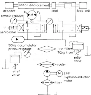
Electrohydraulic servosystems are widely used in con- trol system applications for position or velocity con- trols such as mobile, airborne, and stationary equipment which require servos to convert electrical controls to large mechanical propulsion forces [l-3, 5 , 61. The simulated system in this paper is shown in Fig. 1. It consists essentially of a power cylinder and a servovalve that controls oil flow. Owing to the flow pressure properties and to the load system motion itself, the dynamic characteristic between the power cyl- inder and servovalve is often complex and highly non- linear, which will result in the time-varying of the pressure gain and flow gain obtained from the line- arised hydraulic system for a specified operating point.

linear displacement 3-phase-induction re1 i ef v a l v e motor filter

A

Fig. 1 Schematic diugrani of electrohydraulic velocity control system

Therefore, a linear model used for describing a hydrau- lic system should include unmodelled dynamics. In [2, 31, the authors proposed a model reference adaptive control scheme for the problem of controlling the posi- tion of the system using the linearisation technique for a fixed constant, nominal operating point and consider- ing no external load disturbances. As for the velocity

IEE Proc.-Control Theory Appl., Vol. 143, No. 5. September 1996

control problem, the authors [ 5 ] presented an adaptive model following control scheme to tackle the system with changing operating points and linear load distur- bances. However, since the load disturbances of the hydraulic system depend on the velocity of the piston, and are always nonliinear and time-varying, it is diffi- cult to consider the :stability of the system only with linear load disturbances or with any fixed operating point. Furthermore, it is hard to exhibit good efficiency and performances by using conventional control schemes for the nonlinear hydraulic systems.

In recent years, numerous approaches have been made in the literature towards achieving global stability and convergence of the control system using the indi- rect adaptive control scheme without external persist- ently probing signals [7, 9-13]. In this control scheme, the basic idea is to constitute an on-line estimation algorithm to estimate plant model parameters and then to obtain ii stabilising controller based on the certainty

equivalence principle such that the stability of' the clos- edloop system can be achieved. In general, the external load disturbance always varies in an unknown fashion, although it is bounded, and the unmodeled dynamics exist due 1.0 the fact that the chosen plant model does not give complete descriptions of the controlled plant. So, the estimated model from an on-line estimation can never capture the true: system model, which would push the estimation into poor excitation. It is theriefore bet- ter to obtain an on-line linear model with urimodelled dynamics for use as the basis of control system design by dead-zone technique to avoid the phenomenon of poor excittation [ l l , 15, 16, 18, 241.

In this paper, we propose a certainty equivalence based indirect adaptive contrel (IAC) scheme with self- excitation capability using the pole-placement tech- nique for the problem of controlling the velocity of the hydraulic system sub.ject to unmodelled dynamics and load disturbances. The control scheme is an outgrowth of the work of [16, 18, 241, which can be used to guar- antee global stability of the controlled system without being corrupted by the uncertainties. To estimate the parameters of the plant model, we use the gradient least squares dead-zone estimator [16, 181 to obtain the best curve fitting data on-line. It has been shown that this estimator has monotonic parameter error reduction capability with an easily added norm-bound dead-zone errors given by the plant output and control input his- tories and uncertainti~es. Hence, it can treat a noncon- servative uncertain signal energy bound and give a better transient perfo:rmance of the system. In addition, it is cornputationally efficient and only requires approximately the same memory and computation time as recursive least squares. It is shown that, based on such an effective estimator, a design procedure for syn- thesising the certainty equivalence based ada-ptive con- troller is formulated by using the pole- placement technique, wherein a signal is created and fed back to the control law such that the control scheme has self- excitation capability. Thus, when it is applied to con- trol the velocity of tlhe hydraulic servosysteni, the sta- bility of the closed-loop control system can be achieved without being corrupted by the nonlinearity olf the flow pressure property, the variations of operating points of the hydraulic system, and the load disturbances. A

series of simulations are performed to demonstrate the effectiveness of the proposed scheme. The results show that the proposed scheme is fairly robust to the systems

with uncertainties and also improves performance char- acteristics, as compared with that of the suboptimal PID control scheme with constant feedback gain [4] and that of the adaptive model following control scheme [5].

2

algorithm

2.7 Modelling of the plaint

Consider an uncertain plant P(p) which is described in a stable factor form by

Derivation of the indirect adaptive control

(4)

A

@

'

= [AA,_ 1 . . . AAOABnL-l . . .

AB01

₍₅₎

where p

2

didt, u ( t ) and y ( t ) are the command input and plant output, respectively, and A@) =

@+A,)

...

@+A,)

is a known, strictly Hurwitz polynomial. Moreo- ver, A#@) and B#(p) are the nominal part of the plant, and AA@) and AB@) are the signals which arise because of time variation of system parameters and external load disturbance. The following a priori infor- mation will be assumed about the process:

(Al) A#@) and E#@) are coprime.

(A2) 1/A011 < 6 , V t where

11.11

denotes the usual Eucli- dean norm on Rn+" ancl 6 is a some, known positive constant.

(A3) n and m are known.

The uncertain plant described above can be reformu- lated as

A # ( P ) U f ( t ) = B#(PI'uf(t)

+

W f ( t ) (6) where u k t ) and yAt) are the filtered signals of the com- mand input u ( f ) and plant output y(t), respectively, sat- isfying * ( p ) u " f ( t ) =: ' u ( t ) ( 7 ) NP)Yf(YJ =-

d t )

( 8 ) (9) @ ( t ) = bn-'yf(t). . - w f ( t ) - p " - l u S ( t ) " ' - U " f ( t ) ] (10) and W f ( t ) =

-aoT4(t)

= p n y f ( t )

+

OT$h(t)

2.2 Adaptive

control

algorithm

In the adaptive control system, since 0 is unknown and only the plant input and output are measurable, we are in a position to use the gradient least squares dead- zone estimator to estimate the parameters of the plant model from the plant input and output. Let O ( t ) be an estimate of 0. Since @ ( t ) is constructible in real time, and the parameter estirnate O ( t ) is known at time t,

wf(t) defined in eqn. 9 for each fixed t is estimated according to the following:

w j ( t , T ) =

P"Yf(T)

+

Q"(,+lO)

(11)

= P ( T ) q q T )

+

W f ( T ) 0

5

7 5

t

(la)

where

6(t)

=

e(t)-o.

Let the identification error be defined by

e ( t )

= p n y f ( t ) -

o T ( t ) 4 ( t )

= w f ( t )

+

i T ( t ) $ ( t )

(13)

Since the difference f l ( t ) - O ( ~ ) , x E [0, t ] , is known to the estimator, one can thus construct the functional corre- lation error signal

q ( t , 7 ) = 2 i f ( t . 7)

+

( q t )

- Q ( T ) ) T 4 ( T ) (14)

=

Tr(t)4(7)

+

W S ( T ) 0

5

T

5

t(eqn.12) (15)

To construct an estimation algorithm, it is assumed that

wAt)

and its derivatives satisfy

Ilw(t)//

5

P 4 t ) V t (16) where w(t) = [0 ... 0 pn-'wl{t) ... wj(t)lT, b i is some posi- tive scalar and d ( t ) is defined by

02

P 4 t ) = - P 1 4 t )

+

P2(IUJ(t)l

+

l Y f ( t ) i

+

1) 4 0 )

>

--

01

(17)

where [ 3 , , [j2 > 0 and (3,+(3, < min(A,, ..., A,) for some The gradient least squares algorithm for identifying

8 3

0.

the parameters of the plant model is given by where

@ ( t )

= P a t ) = -r(t)l(t)s(t) (18) t t ( 2 2 ) ( 2 3 ) 0 n -

4 t ) =

S U P

14.11

o < T < t

Proposition 1: [16-18] The estimation algorithm defined by eqn. 18 has the following properties:

(i) Letting ';(t) = dist(O(t), 0 ) where dist(.;)

is

a given distance, then

P(C"t))

5

- 2 ~ ( t ) ~ ( t ) ( l l ~ ( t ) l l C ~ - ~ ~ ~ (~ ) ~ ll ~ (5 0 ~ ) lV t l C I

(24) with equality if and only if pO(t) = 0.

(ii) 'Transient performance:'

p m

[ l l d ~ ) l l C l -

/mI+

llrl(t)llc,dt

L

C2(0)

0

= constant (25) where

[.I'

denotes the positive part.

From qqn. 18, we can make up the estimated polyno- mials .l(O(t),p) and B(O(t),p) for the controlled plant. Let

s(0)

and s ( O ( t ) ) be the Sylvester matrices consti- tuted "by the coefficients of polynomials ( A # @ ) , B#(p)) and .l(O(t),p), B(O(t),p)), respectively. By the coprime- ness of A#@) and B#Q7), there exist two unique polyno- mials

R ( p ) = pn

+

Rn-1pn-l

+

.

. .

+

R i p

+

R,

S ( p ) = s,-lpn-l

+

. ' .

+

SIP

+

so

450

such that

where E@) = p2n

+

!,,-,p2"-'

+

...

+

Eo

is a desired closed-loop characteristic polynomial. Following the assumptions AI-A3 in Section 2.1, the certainty equiv- alence based robust adaptive controller is given by where r f ( t ) = r(t)/A(P) is an external reference input and

T(p) = Tn. ~p"'

+

... +T$+T, which can be selected properly to achieve tracking purpose. Moreover, R(B,, p ) and S(B,, p ) are evaluated from the following:

R(P)A#(P)

+

S ( P ) B # ( P ) = (26

1

N Q O " ( t ) , P ) 7 J f = T ( P ) T f ( t ) - S(Q'Z(t)>P)Yf(t) + n 0 ( t ) (27)

W ( t ) , P ) A ( Q O " ( t , , P ,

+

S ( Q a ( t ) , P ) & w , P ) = E ( P ) (28) and O,(t) and no(t) are evaluated as follows:

If idet(s(fl(t)))i 5 p > 0, then

Q,(t)=O(t) with t=max{$l$

<

t and

1

det(S(Q(6)))l

>

p }

(29) (30) (31) ( 3 2 )

I

no

( t )

=

nl

( t )

+

no2

( t )

n&) = K j i q t ) , n l ( t ) = namax,/T,lT, 0

<

a

<

cc /c

>

0 - T = supl{pnrS(t)pn-lrf(t).

.

T f ( t ) }

Else

Q,(t)

=

e ( t )

no(t) = 0

Note that the initial value O(0) must satisfy Idet(S(O(0)))l > p. It is seen that the adaptive control scheme takes the form of an adaptively tuned linear controller with an additional feedback signal no(t). Also, the reference signal is compensated by the signal n l ( t ) , the control parameters variations are completely removed when idet(s(O(0)))i 5 p, and the effect of the

uncertainties are cancelled by n2(t). The latter produces also the required amount of excitation.

Eqn. 27 can be written as

P " U f ( t ) = - R,-l(Bn(t))pn-lUf(t)- . ' ' -R"(Ba(t))u,f(t)

+Tn-lp"-lTf(t)

+

' ~ ' + T I T f ( t )

- sn-l(Q'Z(t))p"-lYf(t) - " ' - So(Qa(t))Yf(t)

+

no(t)

( 3 3 ) Then the control law eqn. 33 provides pnuJ(t) which together with eqn. 7 allows the computation of the actuator input u (t ) as follows:

u ( t ) = p n 7 r f ( t )

+

X,-lpn-luf(t)

+

' . '

+

X , U f ( t ) (34)

Given the signals y ( t ) and u(t), the filtered signals yj{t), q ( t ) and their differentiations, and the estimate

O ( t ) , the purpose of this paper is to design a certainty equivalence based indirect adaptive control algorithm eqns. 18 and 27 such that the input signal u(t) and out- put signal y ( t ) , and the estimated parameter errors will be uniformly bounded subject to the unmodelled dynamics and load disturbances.

Proposition 2: There exists a positive-scale k l and any unit vector v such that ivr@(t)l / ( d ( t ) ) 2 k l K - p ( t )

where p ( t ) is bounded for all t . The proof is shown in Appendix 7.1.

Proposition 3: The estimated parameter error is uni- formly bounded for all t. The proof follows directly We can now establish the stability of the adaptive

U

11.

control system.

Theorem 1': With thle uncertain dynamics :satisfying eqn. 16, when the adaptive control algorithm eqns. 18 and 27 is applied to the system eqn. 1, it ensures that u(t) and y ( t ) are uniformly bounded for all t.

The proof is very similar to that of Appendix F in [24] and is: therefore, omitted.

From the above analysis, the indirect adapt' ' ive con- troller design procedure is delineated as follows: Step 1: Select the plant model with proper dimension to construct O(t) and @(t)m and a proper filter l/A(p).

Select a stability margin p and O(0) such that Idet(9 Select the characteristic polynomial

E@).

Give the values for $(0), e,,

PI,

p2,

a , K , p, d(0) and

r(4.

Step 2: Update A,,j = 0, 1, ..., n-1, and BjJ == 0, 1, ..., m-1, using, the update law in eqn. 18.

Step 3: Chlculate R(O,(t), p ) and S(O,(t), p ) from eqn. 26 and select 7(p) properly to achieve tracking

purpose.

Step 4: Then the adaptive control law is attained from eqn. 27.

The Steps 2-4 are repeated at each sample time. Remarks: I n Step 3 , if IRo(ea(t))l s E for a small positive

value E, one can freeze ur(t) to keep safe from a very

large control input since the freezing technique [21] is still applie'd.

If the output performance is unsatisfactory, then we can increase the value p to cope with the gadn of the signal corruption and repeat Steps 2-4.

From proposition 2 and theorem 1, if the identifier or the control law g o w s without bound and/or u ( f ) and y ( t ) bllow up, then modify the values a arid K from eqn. 30, and repeat Steps 2-4.

3 Simuilations anid discussions

3.

I

Simulations

A mathematical model for the electrohydraulic velocity

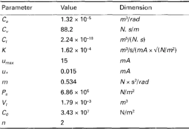
control system was derived in Appendix 7.2. The parameten of the hydraulic servosystem used for simu- lations are: listed in Table 1.

(O(0)))l > IP.

Table 1: Parameters oif electrohydraulic servosptem

Parameter Value Dimension

ca 1.32 x 10 m3/rad C" 88.2 N. slm

c,

2.24 x lO-'O m5/( N. s) K 1.62 x IO4 rn3/sl(mA x t'(Nlm2) ulna, 15 m A U * 0.015 mA m 0.534 N x s2/rad ps 6.86 x IO5 N/m2 vt I .79 10-3 m3 CO 3.43 107 N/m2 n 2

From Table 1, the minimum and maximum values of

Kq and K, in eqn. 51 can be given by 0.07747 5 K q

<_

0.15493

1.27 x

5

K ,

5 2.54

x 1 0 - ~ (35)

IEE Pro( -Coiztiol Theory Appl Vol 143 N o 5 Septemhei 199t'

and thus the parameters of the mathematical model of the electrohydraulic velocity control system in eqn. 54 are

y(t )

+

Ailj(t)

+

Ao%f(t) == Bou(t)

+

~ ( t )

(36) where A. = 174.6736, A , = 166.2256, 492.032 5 Bo 5 984 and w ( t ) = 1.97948 CdyZ(t) -3.7453 Cdy(t)y(t). (i) Step 1: A parametric model of the following form was fitted to the on-line data i o the system:

(37)

m a

( t )

1 P ) / A ( P ) - 6 0 / A ( P ) A ( W ) , P ) / ~ ( P ) (P2

+

AlP

+

A o ) / A ( P )

-

that is, O ( t ) =

[Al

4

k0lT

and @(t) = byAt) y f ( t ) -u{(t)lT. Let the filter 1/A(p) having a roll-off at roughly 20rad/s be given by

1 1

The position of the filter in the simulated system is shown in Fig. 2.

---:

gradient least squares dead-zone algorithm

r-

-

6,

bandpass bandpass

u ( t ) Y ( t )

Fig. 2 Filter.y,/or purumtrr estimution ulgorithm

Letting p = 2.25 x the initial values of the model parameters AI A$ and Bo can be selected as 0.01, 0.02 and 0.015, respectively, such that idet(s(e(0)))l > p. Let the dominant closed-loop poles be placed with a bandwidth of roughly 10radis and with a damping fac- tor of 0.75, and this characteristic polynomial be given z ( p ) = p4

+

65p3

+

1475p2 $- 1 4 3 7 5 ~

+

62500 (39) The required known U priori control parameters used

for simulations are listed in Table 2. by

Table 2: Design parameters

Parameter Value 4 (0) 0 C1 0.1 01 15 P 2 10 U 1 k 12.3 w 1.1 d (0) 1 Y ( t ) 1

(ii) Step 2: Update S ( l ) =

[Al

&

&Ir

using thc update law eqn. 18.

(iii) Step 3: By the certainty equivalence principle, the control parameters R,(O,(t)), Ro(Oo(t)), S,(O,(t)) and 451

10 u ( t ) =.u(t)

+

--n(t)

0.01 0

(42) where h, = 50 and h, = 625 as given in eqn. 38.

A0 B O A1 ... .. ... ~ ... . ~~ ... ~ ... <,',, i ... ~ ~ ... ~ ~ ~ ... ~ ... ... In

2-

0.01 h 0 1 ' " " 0 0.04 0 0 8 012 016 0.20 time, s

Trajectories of control system subject to C,, = 0. velocity output Fig.3

0-0-0 AMFC Y it)

x-x-x suboptimal control scheme

0 0 0 4 008 0.12 0.16 0.20

time, s

Fig.4 Trajectories of control system subject to C, = 0: actuator signal

$2*

I*C In

.

E- 0.01 z1

of

" " " " ' J 0 0.04 0.08 0.12 0.16 0.20 time, s

Trujectories of control system subjecl to C, = 9.8 x IO6: velocity Fig.6

ozrtput y ( t )

x -x-x suboptimal control scheme

*_*-* IAC 0-0 0 AMFC

2-TLE-=7

= J 5 0 0 4 008 012 016 020 time, s OO Fig.7

rignul u ( t ) Trajectories of control syrtem subject to C, = 9 8 x IO6 uctuator *_*-* IAC 482 - O O l l - . ' ' ' ' A I , , I 0 004 008 012 016 020 time, s Fig.8

pczrumeters Trujectorm of control system subject to

C, = 9.8 x IO': system 0 02 E 0 0 1 In

.

<

0 0 004 008 012 016 020 time, s Fig.9

output V ( t ) fiojectoria oJcontrol system subject to C , = 39.6

x IO6: velocity

x-x-x suboptimal control scheme

IAC 0-0-0 A M F C

2-::F

' ' '

--:!

3 5 0 0 0 0 4 008 012 016 0 2 0 time, s Fig. 10 tor signal U *-* * IAC

Tfajeclories o j tontiol system Jubject to

c,

= 39 6 x 10' uctuu-

- ' . O 4 k 004 ' 0.08 ' 0.12 ' 0116 ' 0 10

time, s

Fig. 11

parameter's Trajectories

of contvol system subject to C, = 39.6 x I O 6 - system

Following the design procedure, a series of simula- tion studies are made, for various load disturbances, to evaluate the performance by the proposed scheme. These results are compared with those of the subopti- mal PID controller [4] and that of the adaptive model following control scheme [5]. These simulations are done by a digital computer using the Simnon software package with a step size 0.001s. To investigate the effect of the load disturbance on the hydraulic system, n is chosen to be 2. Throughout the simulations, the reference velocity input is kept at O.O15m/s. The performances of the system with c d = 0, c d = 9.8 x IO6, C, = 39.2 x lo6 and C, = 9 . 8 ~ 1 0 ~

+

0 . 9 8 ~ 1 0 ~ sin(40xt) are illustrated in Figs. 3-5, 6-8, 9-11 and 12-14, respectively. The simulation results are compared to that of the suboptimal controller which has the follow- ing form:

(43) This controller minimises the cost function ISE (inte- gral square error) criterion. The detailed design proce- dure of the suboptimal controller can be found from

[4].

From the design procedure the parameters k,,,

ki

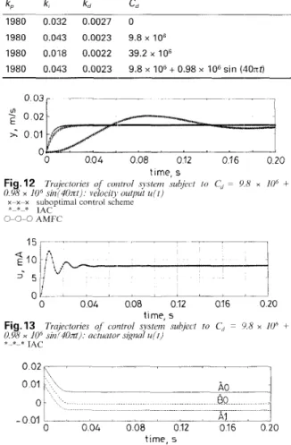
and kd subject to various cases of uncertainties are shown in Table 3.

Table 3: Design parameters for PID controller

1980 0.032 0.0027 0

1980 0.043 0.0023 9.8 x IO6

1980 0.0118 0.0022 39.2 x IO6

1980 0.043 0.0023 9.8 x IO6

+

0.98 x IO6 sin (4Orrt)

5

:::c

0 0 004 008 012 016 020 time, s Fig. 12 0.98 x I O 6 s i n ( 4 0 ~ t ) : velocity output u ( t )

Truiectories of control sys/ein .subjc,c~ lo C, = 9.8 x IO6 t x-x-x suboptimal control scheme

*-*-* IAC 0-0-0 AMFC O I L ’ 1 - LJ--.- -0 0.04 0.08 0.12 0.16 0.20 time, s Fig.13

0.98 x IO6 sin,/40&): actuator s@al u(f)

Truiectories of’ control system subject to CO = ‘9.8 x IO6 +

* .*-* IAC 0.02 0.01 0 - 0 01 Fig.14

0.98 x IO6 .rin(40zt): systent paranwters

0 0.04 0.08 0.12 016 0.20

time, s

Trajectories of control system subject to C,, = 9.8 x IO6 +

The simiilation results are also compared to that of the adaptive model following control (AMFC) scheme [ 5 ] . In the AMFC scheme, the design parameters used for simulations are the same as that in [5] since all con- ditions givmen in eqns. 31, 32 and 41 in [5] are ,satisfied.

3.2

Discussions

The above sirnulatiom indicate that:

(i) For th’e case C, = 0, the velocity responses per- formed by the IAC arid AMFC schemes shown in Figs. 3-5 are almost the same and slightly lag behirid that of the suboptimal PIDl controller. In this case, the response performed by the IAC scheme behaves with a small amount of steady state error, about 0.3‘%1 of the desired value, and a small amount of overshoot since the damping factor of the desired closed-loop charac- teristics is selected as 0.75.

(ii) As to Cd = 9.8 x lo6 shown in Figs. 6-8, the responses -performed by the AMFC scheme arid subop- timal PID controller are observed to be inferior to that of the IAC scheme. /ilso, the response of the subopti- mal PID controller shows large overshoot and oscilla- tion.

(iii) From Figs. 3-1 1, it is also observed that the veloc- ity responses of thie AMFC scheme show slower response (characteristics and that of the suboptimal

controller exhibit large oscillation as the magnitude of the load disturbance increases, However, the responses

of the proposed IAC scheme behave well only with a small amount of undershoot. This feature can be explained as follows. At some time, if the determinant

o f the Sylvester matrix 3 0 ( t ) > is smaller than the pre- specified controllable margin p, then the estimate is replaced by the last past one which we can use to design a stabilising controller, and the exciting signal is fed back to the cont:rolled plant simultaneously. Finally, when the excitation becomes poor again, the estimate still can be used to design the corresponding stabilising controller.

(iv) As to Cd = 9.8 x IO6

+

0.98 x IO6 sin(40mt) shown in Fig. 6, the response of the velocity performed by the IAC scheme shows more satisfactory results for the dis- turbance with unknown as well as time-varying charac- teristics than that of the AMFC scheme and the suboptimal PID controller.

(v) From the simulation results, because there exist par- ametric uncertainty and disturbance, the estimated parameters obtained from estimation algorithm will not approach the true values but when used for designing the adaptive controller, the controlled system can be stabilised all the time.

(vi) From the above discusslons, the proposed IAC scheme can be a promising way to tackle the problem of controlling thc velocity of hydraulic servosystems subject to time-varying external velocity-dependent load disturbances.

4 Conclusion

In this paper, we have proposed a robust certainty equivalence based adaptive control scheme with self- excitation capability, which is an outgrowth of the work of [16, 18, 241, to the problem of controlling the velocity of electrohydraulic servosystems subject to unmodelled dynamics and external load disturbance. The estimator used for ideritifying the parameters of the plant model is similar to that proposed by [16-181. It is shown that the proposed adaptive control scheme using the certainty equivalence principle and pole placement technique can guarantee the boundednesses of the input and output of the controlled plant. From the simulation results, the proposed adaptive control scheme is fairly robust to the systems with unmodelled dynamics and unknown as well as time-varying load disturbance, as compared with that of the suboptimal PID control scheme arid that of the AMFC scheme.

5 Acknowledgment

The authors would like to thank the reviewers for their constructive comments.

6 References

1 MERRITT, H.E.: ‘Hydraulic conlrol systems’ (Wiley, New York,

1967)

2 PORTER. B.. and TATNALL. M.L.: ‘Performance characteris-

tics of dn addptivc hydrdulic servo-mechanism’, Int J Control,

1970, 11, pp 741-757

3 KULKARNI. M M

.

TRIVEDI. D B . and CHAN-

DRASEKHAR, J.: ‘An adaptive control of an electro-hydraulic position control system’. Proceedings of American Control Con-

ference, 1984, pp 443-448

4 Y U N J S , a n d CHO, H S ‘A ,uboptimal d e w p approach to

the ring diameter control for ring rolling processes’, Truns.

ASME. J . DJW. Syst. Meus. Conlrol, 1985, 107, pp. 207-212 5 YUN, J.S., and CHO, H.S.: ‘Adalptive model following control of

electrohydraulic velocity control systems subjected to unknown

disturbances’, IEE Proc. D , 1988, 135, (2), pp. 149-156

LEQUOC, S., CHENG, R.M.H., and LIMAYE, A.: ‘Investiga-

tion or an electrohydraulic servovalve with tunable return pres-

sure and drain orifice’, Trans. ASME, J. Dyn. Sysl. Meus.

Control. 1987. 109

7.2

Derivation o f

mathematical

mode/ Referring to Fig, and orifice law, the load flow rate

(0,)

of the servovalve to the actuator input current (U)

KREISSELMEIER, G.: ‘An indirect adaptive controller with a

self-excitation capability’, IEEE Trans. Autom. Control, 1989, AC-

KREISSELMEIER, G.: ‘Adaptive observers with exponential

isgiven by [I, 5 , 61

34, ( 5 ) , pp. 524-528 Ql =

K u J P ,

- sigii(u)Pl

(47)

rate of convergence’, IEEE Trans, Autom, Control, 1977, AC-22, where is the ‘Onstant, 5‘ is the pressure,

( I ) , VU. 2-8 Pi is the load pressure across the cylinder, and

KREkSELMEIER, G., and SMITH, M.C.: ‘Stdbk adaptive reg-

ulation of arbitrary nth-order plants’, ZEEE Trans. Autom. Con-

trol, 1986, AC-31, (4), pp. 299-305

10 GIRI, F., M’SAAD, M., DION, J.-M., and DUGARD, L.: ‘On

tlie robustness or discrete-time adaptive linear controller’. Pre-

sented at 1988 Proceedings IFAC Workshop Robust Adaptive Control, Newcastle, Australia, Aug. 1988

11 GIRI, F., M’SAAD, M., DION, J.-M., and DUGARD, L.: ‘On

the robustness o l discrete-time adaptive (linear) controllers’, Auto-

matica, 1991, 27, ( I ) , pp. 153--159

12 ELLIOTT, H., CRISTI, R., and DAS, M.: ‘Global stability of

adaptive pole placemerit algorithms’, IEEE Trans. Autom. Con-

trol, 1985, AC-30, pp. 348-356

13 PENG. H.-J.. and CHEN. B.-S.: ‘A robust indirect adantive ree-

ulatioil algorithm with self-excitation capability’, I E k E Tran:.

Autom. Control, 1993, AC-38, (2)

14 ELLIOTT, H.: ‘Direct adaptive pole placement with application

to nonminimum uhase systems’. IEEE Trans. Autom Control.

1982. AC-21. no. 720-722’

15 ASTROM, K:f., and WITTENMARK, B.J.: ‘Adaptive control’

16 KRAUSE. J.M., and KHARGONEKAR, P.P.: ‘A comparison (Addison-Wesley Publishing Company, 1989) of classical stochastic estimator and deterministic robust kstima-

tion’, IEEE Trans. Autom. Control, 1992, AC-37, (7), pp. 994-

1000

17 KRAUSE, J.M.; STEIN, G., and KHARGONEKAR, P.P.:

Toward practical adaptive control’. Proceedings of the American

Control Conference, June 1989, pp. 993-997

18 KRAUSE, J.M., and KHARGONEKAR, P.P.: ‘Parameter iden-

tification in the presence of nonparametric dynamic uncertainty’,

Autornatica, 1990, 26, (I), pp. 113-123

19 ASTROM, K.J.: ‘Robustness of a design method based on

assignment of poles and zeros’, IEEE Truns. Autom. Control,

20 MILLER, R.K., and MICHEL, A.N.: ‘Ordinary differential equations’ (Academic, New York, 1982)

21 ANDERSON, B.D.O., and JOHNSTONE, R.: ‘Global adaptive

pole positioning’, IEEE Trans. Autoni. Control, 1985, AC-30, (1),

22 HA”, W.: ‘Stability of motion’ (Springer-Verlag, New York,

1967)

23 VIDYASAGAR, M.: ‘Nonlinear systems analysis’ (Prentice-Hall, 1993)

24 MIDDLETON, R.H., and GOODWIN, G.C.: ‘Digital control

and estimation: A unified approach’ (Prentice-Hall International, Inc., 1990)

25 GOODWIN, G.C., and TEOH, E.K.: ‘Persistency of excitation in

tlie presence of possibly unbounded signals’, IEEE Trans. Autom.

Control, 1985, AC-30, pp. 595-597

1980, AC-25, ( 3 ) , pp. 588-591

pp. 11-22

7 Appendix

7.1 Proof of Proposition 2 From [14] and eqn. 27, we have

QT(t)S(@)Ld(t) = T ( P ) T f ( t ) - S ( Q , ( t ) , P ) W . f ( t ) + no(t)

(44) where e C ( 4 = [R,-,(%(t)>

’..

R,(%,(t))

s,-,(%(t>>

...

SO(O,(t))lT and L is a known full rank matrix. Since OCr(t)S(o)L is not a zero vector, we can take vT =

LTSr(@)E!,(t) / ~ ~ L T S T ( @ ) € ) , ( t ) ~ ~ . Dividing both sides of eqn. 44 by lILTST(o)€tC(tjll and pd(tj results in

IVT4(t)l kllnz(t)l k l / S ( Q a ( t ) > P ) ~ ~ f ( t ) l - k ; p ~ d t ) l P $ t ) P 4 t ) / a t ) P a t )

O < k l < O o

Since iT(p)rdt)l 5 nmaxilT,17 is bounded and, -from eqns. 16, 27 and 28, the signal IS(8,(t),p)wj(t)l / p d ( t ) is also bounded, we have

(45)

where p(t) = (k,lS(E!,(t),p>wdt)l

+

(cr-kl)nmaxj/TjIF)l (p

d(t))

is bounded.

sign(u) = I , for U-> 0, sign(u) = -1, for U - < 0. For the application of the adaptive control, the linearised sys- tem of eqn. 47 is obtained for an arbitrary operating point in the following:

where K4 = Kv‘(P,,-sign(u*)P,*) is the flow gain, K, =

Klu*l/{v‘(/(P,~-sign(u*)P~*)} the pressure coefficient and ‘*’ means the nominal operating point. The continuity equation of the servovalve and the cylinder chamber is given by

Q i 1 K,u - K,Pl ₍₄₈₎

Q1

= Cad

+

C I B

+ (3)

Ijl

4co (49)

where C, is the piston ram area, C, is the total leakage coefficient, V, is the total volume of the valve and the cylinder chamber, CO is the bulk modulus of the oil, and $ is the velocity of the piston. To determine the minimum and maximum values of the parameters Kq and K, the following physical consideration can be uti- lised:

where C, is an arbitrary positive number less than 1 and is chosen as 213 for the reason that power elements are sized such that PI does not exceed 213P, for the maximum loads normally expected. Thus, the mini- mum and maximum values of Kq and K, can be obtained as

which imply that only the bounds of the magnitudes of Kq and K, are known. It is assumed that the magni- tudes of Kq and K,. are slowly time varying within the bounds. Under the assumption that Coulomb friction between the piston and sleeve is negligible, the equation of motion of the piston is given by

where m is the total mass of piston and load, and C,, is the viscous damping coefficient. It is assumed that the external load disturbance, Fl(Q(t)), is differentiable with

Q ( t ) and is frequently given by

where Cd = 6 F I / 6 ~ ( t ) l i * ( t ) and n is a positive integer number. The above equation indicates that the load

disturbance depends on the velocity of the piston,

which acts as a nonlinear damper whose damping coef- ficient varies with the velocity

[SI.

Hence, letting y ( t ) =

W(t), we obtain the following linear differential equa- tion with parametric uncertainties and external load disturbance:

(54) where C , = m/(4C0), K, = K,

+

C,, A. = (C:

+

K,C,)/

C,Pl = m&t)

+

C,&t)

+

f i ( & t ) ) (52)

F1(4(t))

= C,G”(t) (53)

y ( t )

+

Ailj(t)

+

A o y ( t ) = @ u ( t )

+

~ ( t )

(Cbm), AI = (Kern + CbCv)/(Chm>, BO (CaKq)l(Ci~m)> w(t> = -Cd,Y”(t> - Cd2y”-’(t)Av(t>, Cdl = KeCdl(Cbm),

c d z = nCdIrn and n 1.

IEE Proc.-Control Theory Appl., Vol 143, No. 5, September 1996