電解質溶液於細孔內之電動力流動(2/3)

行政院國家科學委員會專題研究計畫 期中進度報告

電解質溶液於細孔內之電動力流動(2/3)

期中進度報告(精簡版)

中 華 民 國 96 年 05 月 13 日

摘要

本計畫對電解質溶液受到外加切線方向溶質濃度梯度之作用下，沿一帶

電孔壁表面吸附帶電高分子層的平板形孔隙內之穩態擴散滲透流動進行理論

探討。其中帶電高分子層的電荷與流動阻力密度為均勻分布，離子與溶劑皆

可自由穿透，且帶電高分子層與電雙層的厚度可為任意值。使用

Debye-Huckel

近似，電位分布可藉由求解線性化後的

Poisson-Boltzmann 方程式而得到，至

於由外加電解質濃度梯度所產生的巨觀電場和流體流速分布可藉由求解修正

後的

Navier-Stokes/Brinkman 方程式而得到。研究結果顯示，帶電高分子層與

電雙層中軸向誘導電場之徑向分布，和帶電高分子層與電雙層外主體誘導電

場間差異的效應，在一般情況下對流體速度的影響相當顯著。而帶電高分子

層的存在亦可大幅改變孔隙內之擴散滲透流動現象。

關鍵詞： 擴散滲透流動，吸附帶電高分子層的孔隙，任意電雙層厚度

Abstract

The steady diffusioosmotic flow of an electrolyte solution in a fine capillary slit with each of its inside walls covered by a layer of adsorbed polyelectrolytes is analytically studied. In this solvent-permeable and ion-penetrable surface charge layer, idealized polyelectrolyte segments are assumed to distribute at a uniform density. The electric double layer and the surface charge layer may have arbitrary thicknesses relative to the gap width between the slit walls. The Debye-Huckel approximation is used to obtain the electrostatic potential distribution on a cross section of the slit. The macroscopic electric field induced by the imposed electrolyte concentration gradient through the slit is determined as a function of the lateral position rather than taken as its constant bulk-phase quantity. Explicit formulas for the fluid velocity profile are derived as the solution of a modified Navier-Stokes/Brinkman equation. The effect of the lateral distribution of the induced axial electric field in the slit on the diffusioosmotic flow is found to be of dominant significance in most practical situations and to drive the fluid towards the end of higher electrolyte concentration. The existence of the surface charge layers can lead to a quite different diffusioosmotic flow from that in a capillary with bare walls.

1. Introduction

The flow of electrolyte solutions in a small pore with a charged wall is of much fundamental and practical interest in various areas of science and engineering. In general, driving forces for this electrokinetic flow include dynamic pressure differences between the two ends of the pore (a streaming potential is developed as a result of zero net electric current) and tangential electric fields that interact with the electric double layer adjacent to the pore wall (electroosmosis). Problems of fluid flow in pores caused by these well-known driving forces were studied extensively in the past century [1-8].

Another driving force for the electrokinetic flow in a micropore, which has commanded less attention, involves tangential concentration gradients of an ionic solute that interacts with the charged pore wall. This solute-wall interaction is electrostatic in nature and its range is the Debye screening length κ−1 (defined right after Eq. (3)). The fluid motion associated with this mechanism, known as “diffusioosmosis”, has been analytically examined for solutions near a plane wall [4, 9-12] and inside a fine capillary [13-16]. Electrolyte solutions with a concentration gradient of order 100 kmol/m4 (= 1 M/cm) along solid surfaces with a zeta potential of order kT/e (~25 mV; e is the charge of a proton, k is the Boltzmann constant, and T is the absolute temperature) can flow by diffusioosmosis at velocities of several micrometers per second.

Although the basic relationships involved in electrokinetic phenomena were derived mainly by using the traditional model of plain distribution of surface charges, quite a number of investigations have applied these phenomena to the study of the effects of polyelectrolyte adsorbates. The electroosmotic flows in capillaries with thin polymer layers on the inside walls were theoretically examined for the cases of a slit [17, 18] and a tube [19] with thin double layers. On the other hand, analytical formulas for the electroosmotic velocity profile of electrolyte solutions on the cross section of a capillary with its inside wall covered by a finite

layer of adsorbed polyelectrolytes were obtained by solving the linearized Poisson-Boltzmann equation for the case of an arbitrary value of κ or hR κ , where R is the radius of a capillary

tube and h is the half thickness of a capillary slit [20]. Recently, the diffusioosmotic flow of a symmetric electrolyte solution in a fine capillary slit bearing adsorbed polyelectrolytes on its inside walls was theoretically investigated for the case of small potentials or low fixed-charge densities, and an analytical formula for the fluid velocity profile on the cross section of the slit was obtained [21]. In this study, however, the effect of lateral distributions of the counter-ions and co-ions on the local macroscopic electric field induced by the imposed electrolyte concentration gradient in the axial direction, which can be important, was neglected.

In this report we present an analysis of the steady diffusioosmosis of an electrolyte solution with a constant imposed concentration gradient through a capillary slit bearing permanently adsorbed or covalently bound polyelectrolytes on its inside walls. The charge and segment densities of the adsorbed polymers are assumed to be uniform throughout the surface charge layer, and the Debye-Huckel approximation for the electrostatic potential is employed. However, no assumptions will be made about the thickness of the electric double layer or the thickness of the surface charge layer relative to the gap width between the slit walls, and the lateral distribution of the induced axial electric field is allowed. We shall derive explicit formulas for the local and average fluid velocities due to the application of an electrolyte concentration gradient along the slit walls. These results show that the effect of the deviation of the induced axial electric field in the slit from its bulk-phase quantity on the diffusioosmotic velocity of the fluid is dominantly significant in most practical situations.

2. Electrostatic potential distribution

We first consider the electrostatic potential distribution in the fluid solution of a symmetrically charged electrolyte on a cross section of the narrow channel between two large

identical parallel plates of length L at separation distance 2h with h<< , as illustrated in Fig. L 1. Each of the inside walls of the capillary slit is coated with a layer of adsorbed, charged polymers in equilibrium with the surrounding solution of a symmetrically charged electrolyte. The polymer layer is treated as a solvent-permeable and ion-penetrable surface charge layer of constant thickness in which fixed-charged groups of valence q are distributed at a uniform density N. (Experimental values for human erythrocytes [22], rat lymphocytes [23], and grafted polymer macrocapsules [24] indicate that d ranges from 7.8 nm to 3.38

b h d = −

m

μ and N can be as high as 0.03 kmol/m3, depending on the pH and ionic strength of the electrolyte solution.) The prescribed electrolyte concentration gradient is a constant along the axial (z) direction in the capillary, where is the linear concentration distribution of the electrolyte in the bulk solution phase in equilibrium with the fluid inside the slit. Since the electrolyte ions can diffuse freely along the capillary (inside and outside the surface charge layers), there exists no regular osmotic flow of the solvent. It is assumed that

, where is set at the midpoint through the capillary slit. Thus, the variation of the electrostatic potential (excluding the macroscopic electric field induced by the prescribed electrolyte gradient, which will be discussed in the next section) and ionic concentrations in the slit with the axial position is negligible.

∞ ∇n ) (z n∞ 1 ) 0 ( / | |∇n∞ n∞ << L z =0

Owing to the planar symmetry of the system, we need consider only the half region , where y is the distance from the median plane between the slit walls in a normal direction. If h y ≤ ≤ 0 ) ( y

ψ represents the electrostatic potential at the position y relative to that in the bulk solution and and denote the local concentrations of the cation and anion, respectively, of the symmetric electrolyte with valence Z (which is positive), then Poisson’s equation gives

) , ( zy n₊ n₋( zy, ) 4π { [ ( ,0) ( ,0)] ( ) } d d 2 2 qN y H y n y n Z e y + − − = _{+ −} ε ψ . (1)

Here, H( y)is a unit step function which equals unity if b< y<h, and zero if 0≤ y<b;

r 0

π 4 ε ε

ε = , where ε_r is the relative permittivity of the electrolyte solution which is assumed to be constant and ε₀ is the permittivity of a vacuum. The local concentrations n₊ and n₋ can also be related to the electrostatic potential ψ by the Boltzmann equation,

exp( )

kT Ze n

n_± = ∞ _m ψ . (2)

Substitution of Eq. (2) into Eq. (1) leads to the well-known Poisson-Boltzmann equation. For small values of ψ (or Zeψ kT <<1, known as the Debye-Huckel approximation), the Poisson-Boltzmann equation can be linearized and Eq. (1) becomes

ε ψ κ ψ qeN y H y π 4 ) ( d d ₂ 2 2 − = , (3)

where κ =[8π(Ze)2n∞(0)/εkT]1/2 is the Debye screening parameter. The boundary conditions for ψ are

( =0)= 0 d d y y ψ , (4a) ψ(y =b−) =ψ(y =b+), (4b) ( ) d d ) ( d d ₌ − _{= =} + b y y b y y ψ ψ , (4c) ε σ ψ 4π ) ( d d = = h y y . (4d) Equations (4b) and (4c) are the continuity requirements for ψ and dψ/dy at the outer edge

of the surface charge layer. Equation (4d) is the Gauss condition at the capillary wall, with σ equal to the surface charge density of the bare wall.

The solution to Eqs. (3) and (4) is Acosh( y) Ze kT _κ ψ = , if 0≤ y ≤b, (5a) [Bcosh( y) Csinh( y) N] Ze kT _{+ +} = κ κ ψ , if b≤ y ≤h, (5b) with ) sinh( ) sinh( h d N A κ κ σ + = , (6a)

) sinh( ) sinh( ) cosh( h b h N B κ κ κ σ − = , (6b) C = Nsinh( bκ ), (6c)

where σ =4πZeσ /εκkT and N =4πZe2qN/εκ2kT . Evidently, the electric potential given by Eq. (5) is correct to the first orders of the dimensionless fixed-charge densities σ and N . Note that the parameter N can also be viewed as the nondimensionalized Donnan potential

[18, 25] of the surface charge layer in the Debye-Huckel approximation.

If the boundary condition (4d) for the case of constant surface charge density is replaced by the boundary condition for the case of constant surface potential,

ψ(y= )h =ζ , (7)

then the solution in the form of Eq. (5) is also valid to the first orders of ζ and ,N with ) cosh( ] 1 ) [cosh( h d N A κ κ ζ + − = , (8a) ) cosh( ] 1 ) sinh( ) [sinh( h b h N B κ κ κ ζ − + = , (8b)

where ζ =Zeζ kT is the dimensionless surface potential, and is still given by Eq. (6c).

By using Eqs. (4d), (5b), (6c), and (8b), it can be found that the relation between C

ζ and σ for arbitrary values of N , κ and bh, κ under the Debye-Huckel approximation is

σ cosh(κh)=(ζ −N)sinh(κh)+Nsinh(κb). (9)

When there is no polyelectrolyte adsorbed on the walls of the capillary slit, or when the adsorbed polymer layer is uncharged, one has N =0. Then, Eqs. (5), (6), and (8) reduce to

) cosh( 0 y A Ze kT _κ ψ = , (10) where ) sinh( 0 h A κ σ = (11a)

for the situation of constant surface charge density, and ) cosh( 0 h A κ ζ = (11b)

for the situation of constant surface potential (B= A= A₀ and C =0).

Then, Eqs. (5), (6), and (8) reduce to ] ) cosh( [B₁ y N Ze kT ₊ = κ ψ , (12) where ) sinh( 1 h B κ σ = (13a)

for the situation of constant surface charge density, and ) cosh( 1 h N B κ ζ − = (13b)

for the situation of constant surface potential (A−N =B=B₁ and C =0).

3. Induced electric field distribution

Since the ionic concentrations n₊ and n₋ in the capillary slit are not uniform in both axial and lateral directions, their prescribed gradients in the axial direction can give rise to a “diffusion current” distribution on a cross section of the slit. To prevent a continuous separation of the counter-ions and co-ions, an electric field distribution along the axial direction arises spontaneously in the electrolyte solution to produce another electric current distribution which exactly balances the diffusion current [4, 10, 26].

)

(z ( y)

Ε

If the electrolyte solution is dilute, the flux of either ionic species is given by the Nernst-Planck equation, )] ( [ E J_± =− _± ∇ _± ± n_± ∇ψ − kT Ze n D , (14)

where the principle of superposition for the electric potential is used, and and are the diffusion coefficients of the cations and anions, respectively, which are assumed to be constant both inside and outside the porous surface layer. In order to have no current arising from the cocurrent diffusion of the cations and anions, one must require that

+

D D₋

J J

J₊ = ₋ = . Applying this constraint to Eq. (14), we obtain

) 0 ( ) ( _∞ ∞ − + − + ∇ + − = n n G G G G Ze kT E , (15)

where ) exp( kT Ze D G_± = _{± m} ψ . (16)

The positive coefficients G₊ and G₋ defined by the above equation reflect the fact of an increase in the axial diffusive flux of the counter-ions and a decrease in the flux of the co-ions inside the electric double layer. Substitution of Eqs. (15) and (16) into Eq. (14) leads to a net flux distribution of the electrolyte in the slit,

, (17) ∞ ∇ − = D n J

where the position-dependent net diffusivity is

− + − + + = G G G G D 2 . (18)

Equation (15) and (17) show clearly that both and are collinear with , which is in the axial direction.

E J ∇n∞

For small values of ψ , a Taylor expansion applies to Eq. (16), and Eqs. (15) and (18) can be expressed as ) 0 ( )] ( ) 1 ( [ − − 2 + 2 ∇_∞ ∞ = n n O kT Ze Ze kT _{β β} ψ _ψ E (19) and )] ( 1 [ 2 _β ψ _ψ2 O kT Ze D D D D D + + + = − + − + _{, (20)} where − + − + + − = D D D D β . (21)

Obviously, −1≤β ≤1. Note that, even if the cation and anion diffusion coefficients are identical (i.e., β =0), the O(ψ) term in Eq. (19) for the induced electric field still exists

(due to the adsorption of the counter-ions and depletion of the co-ions near the slit walls) and equals . In a previous study of the diffusioosmosis of electrolyte solutions in a capillary slit with each of its inside walls covered by a layer of adsorbed polyelectrolytes [21], only the first term in the brackets of Eq. (19) was considered for E (the bulk-phase

E ) 0 ( / ∞ ∞ ∇ −ψ n n

electrostatic potential ψ =0 is taken everywhere), and thus, the effect of the lateral distribution of the induced electric field on the fluid velocity was excluded.

4. Fluid velocity distribution

We now consider the steady flow of an electrolyte solution in a capillary slit with each of its inside walls coated with a layer of charged polymers under the influence of a constant concentration gradient of the electrolyte prescribed axially. The momentum balances on the Newtonian fluid in the y and z directions give

0 d d ) ( − = + ∂ ∂ − + y n n Ze y p ψ ; (22) ( ) ( )E d d 2 2 − +− − ∂ ∂ = − Ze n n z p fu y H y u η . (23)

Here, u(y) is the fluid velocity profile (satisfying the equation of continuity for an incompressible fluid) in the direction of decreasing electrolyte concentration (i.e., direction of

), p(y, z) is the pressure, is the macroscopic electric field induced by the applied concentration gradient of the electrolyte given by Eq. (15) or (19),

∞ ∇

− n E( y)

η is the viscosity of the fluid, and f is the hydrodynamic friction coefficient in the polymer layer per unit volume of the fluid; both η and f are assumed to be constant. Equation (23) is the Navier-Stokes/Brinkman equation modified by adding a term of electrostatic force.

The boundary conditions for u are ( 0) 0 d d _{= =} y y u , (24a) u(y =b−) =u(y =b+), (24b) ( ) d d ) ( d d ₌ − _{= =} + b y y u b y y u , (24c) 0 ) (y = h = u . (24d)

boundary of the surface charge layer. In Eq. (24d), we have assumed that the shear plane coincides with the surface of the bare wall.

After the substitution of Eq. (2) for n_± into Eq. (22) (based on the assumption that the equilibrium lateral ionic distributions are not affected by the axially induced electric field ) and the application of the Debye-Huckel approximation, the pressure distribution can be determined, with the result correct to the second orders of

E σ (or ζ ) and N as = ₀ + ∞( )(Ze)2{[ψ(y)]2 −[ψ(0)]2} kT z n p p . (25)

Here, is the pressure at the median plane between the slit walls, which is a constant in the absence of applied pressure gradient, and the electric potential distribution

0 p ) ( y ψ is given by Eq. (5).

Substituting the ionic concentration distributions of Eq. (2), the electrostatic potential distribution of Eq. (5), the pressure profile of Eq. (25), and the induced electric field profile of Eq. (19) into Eq. (23), and solving for the fluid velocity subject to the boundary conditions in Eq. (24), we obtain _{1 2} 2 ₃ * ₄(1 ) 1 8 1_{Φ β Φ} Φ β + − − = U u , (26) where ) ( ) tanh( ) ( ) ( sech ) ( ) ( ) ( _{1 2 2 0} 1 b g y g b d g h d g b g_{i i i i i} i κ κ κ λ κ λ κ Φ = − − + − , if 0≤ y≤b, (27a) ) ( )] sinh( ) ( ) cosh( ) ( )[ ( sech d g_i2 h y b g_i0 b h y g_i2 y i λ κ λ λ κ λ λ κ Φ = − − − − , if b≤ y≤h, (27b)

for 1, 2, and 3. In the above equations, , which is a characteristic value of the diffusioosmotic velocity, the functions , , and are defined by Eqs. (A1)-(A3) in the appendix, and

= i U∗ =2kT |∇n∞ |/ηκ2 ) ( 0 x g_i g_i1(x) g_i2(x) 2 1 ) / ( η

λ= f . The parameter 1/λ has the dimension of length and the square of it is the so-called Darcy permeability of the porous medium, which is related to the pore (or segment) size and porosity and characterizes the

dynamic behavior of the viscous fluid in it. For the surface charge layers of human erythrocytes [18], rat lymphocytes [23], and grafted polymer microcapsules [24], experimental data of 1 range from 1.35 to 3.7 nm. λ

The definition of the average fluid velocity over a cross section of the capillary slit is u =

h

1

∫

0 u(y)dy. (28)

Substituting Eqs. (26) and (27) into the above equation and performing the integration, we obtain _{* 1 2} (1 2) ₃ 4 1 8 1 _{Φ β Φ} Φ β + − − = U u , (29) with ) ( )] tanh( ) sech( b [ 1 )] ( ) ( [ _{1 2} d d g ₂ h h b g b g h b i i i i κ κ _λ λ λ λ κ Φ = − + + ) ( ) ( ) ( 1] ) sech( ) tanh( [ 1 2 1 0 b s b s b g d d b h λ λ λ i κ i κ i κ λ − + − − − , (30)

where the functions ( ) and ( ) are defined

by Eqs. (A5) and (A6). ) ( 1 x s_i =

∫

∫

The function Φ₁ in Eqs. (26) and (29) represents the first orders of σ (or ζ ) and N , while the functions Φ₂ and Φ₃ denote the second orders. As it is well known, the diffusioosmosis of an electrolyte solution in a capillary pore results from a linear combination of two effects: “chemiosmosis” due to the nonuniform adsorption of counter-ions and depletion of co-ions in the electric double layer over the charged surface and “electroosmosis” due to the macroscopic electric field generated by the imposed concentration gradient of the electrolyte given by Eq. (15) or (19). The terms in Eqs. (26) and (29) involving the functions Φ₁ and

3

Φ represent the contribution from electroosmosis, while the remainder terms (containing the function Φ₂) are the chemiosmotic component. Note that additional second-order terms caused by electroosmosis may exist if the electrolyte is not symmetric.

0 =

λ , and the potential profile in the slit is given by Eq. (10). Then, Eqs. (27) and (30) reduce to ) ( ) ( ₁ 1 h g y g_{i i} i κ κ Φ = − ; (31) ) ( ) ( ₁ 1 h s h g_{i i} i κ κ Φ = − . (32)

In the functions g_i1 and s_i1 for this simple case, we take A= A₀, which was defined by Eq. (11). Equations (31) and (32) agree with the result obtained in a previous article [16], in which only the case of a capillary with bare walls is examined. It can be found by a comparison between Eq. (30) and Eq. (32) that the structure of the surface charge layer can result in an augmented or a diminished fluid velocity relative to that in a capillary with bare walls, depending on the characteristics of the electrolyte solution, of the surface charge layer, and of the capillary.

For the case of a capillary slit coated with an uncharged polymer layer at each of its inside walls, Eq. (10) for the potential distribution is also applicable and the fluid velocity can be evaluated from Eqs. (26)-(30) by setting

) 0 (N = 0 = N , ,B= A= A₀ and C =0.

When λ →∞ (very high segment density), the resistance to the fluid motion inside the surface charge layer is infinitely large. For this limiting case, g_i0(x)=g_i2(x)=0, and Eqs. (27) and (30) reduce to Φ_i =g_i1(κb)−g_i1(κy), if 0≤ y ≤b, (33a) Φ_i =0, if b≤ y ≤h; (33b) ) ( ) ( ₁ 1 b s b g h b i i i κ κ Φ = − . (34)

Equation (33) shows that the fluid flow in the surface charge layer disappears and the velocity profile of the remaining fluid is similar to that in a polymer-free capillary slit of half thickness b with a modified surface charge density or surface potential at the wall.

When λ →0 (very low segment density), the adsorbed polymers do not exert resistance to the fluid motion in the capillary channel. In this limit, Eqs. (27) and (30) become

Φ_i =g_i1(κb)−g_i1(κy)+g_i3(κb), if 0≤ y ≤b, (35a) Φ_i = g_i3(κy), if b≤ y ≤h; (35b) ) ( ) ( )] ( ) ( [g₁ b g ₃ b s₁ b s₃ b h b i i i i i κ κ κ κ Φ = + − + , (36)

where the functions g_i3(x) and s_i3(x) (=

∫

x gi x x h

κ

κ

3( )d / ) are defined by Eqs. (A7) and

(A8). If the adsorbed polymers are uncharged (N =0), the above expressions for the fluid

velocity again reduce to Eqs. (31) and (32).

When the capillary slit is filled with the adsorbed polymers, one has d =h and b=0, and the potential distribution in the slit is given by Eq. (12). Then, Eqs. (27) and (30) reduce to

( ) ) cosh( ) cosh( ) ( ₄ 4 g y h y h g_{i i} i _λ κ λ κ Φ = − ; (37) ) ( ) tanh( ) ( ₄ 4 s h h h h g_{i i} i _λ κ λ κ Φ = − , (38)

where the definitions of the functions and ( ) are given by Eqs. (A9) and (A10).

) ( 4 x g_i s_i4(x) =

∫

5. Results and discussion

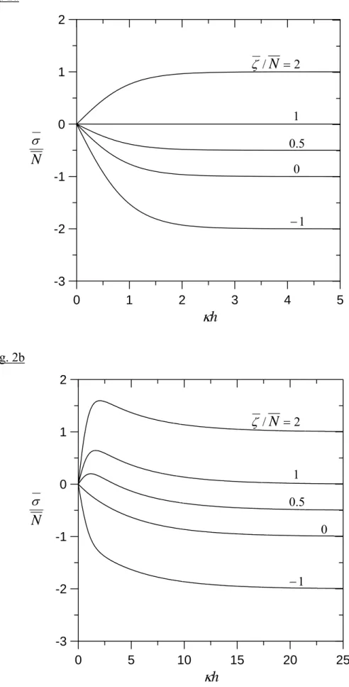
For the system of an electrolyte solution in a capillary slit bearing adsorbed polyelectrolytes on its inside walls, the surface charge density of the wall, the surface potential of the wall, the fixed-charge density in the polyelectrolyte layer, and the electrokinetic dimensions of the system are related by Eq. (9). Figs. 2(a) and (b) show the results of the ratio

N /

σ for the case of and for the case of a finite value of (=0.8), respectively, as functions of

0 /h=

b b/ h h

κ for several values of the ratio ζ /N . It can be seen that σ/N =0 as 0

= h

κ and σ/N =ζ /N −1 as κh→∞, regardless of the values of ζ /N and . For

the special case with and

h b / 0

/h=

b ζ /N =1, the potential in the polyelectrolyte-filled

capillary equals the Donnan potential everywhere, and σ /N =0 at any value of hκ . For the other cases with b/h=0, σ has the same sign as ζ −N and the magnitude of σ/N

increases monotonically with an increase in hκ for a constant value of ζ /N. For the case

with a finite value of b /h, σ/N is negative and its magnitude is still a monotonic increasing function of hκ if ζ /N ≤0, but the dependence of σ/N on hκ may not be monotonic if

0 /N >

ζ .

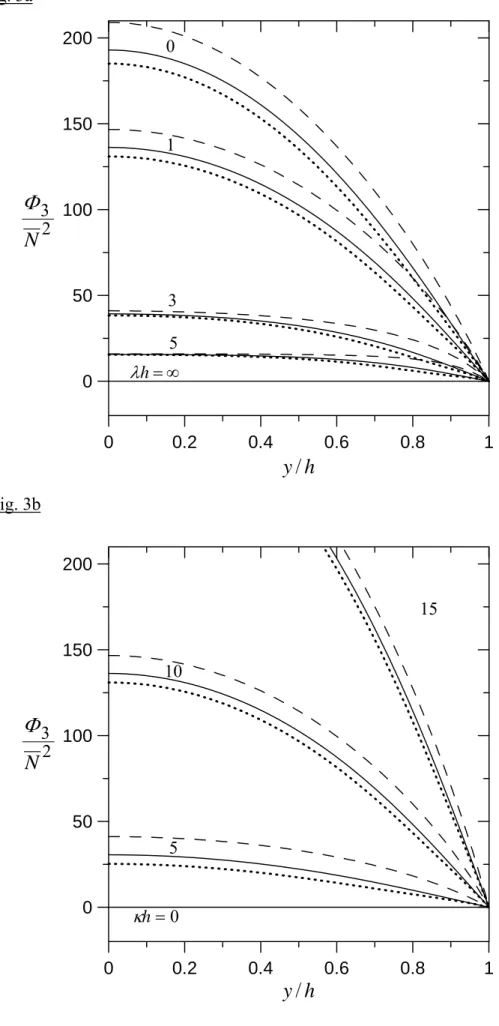
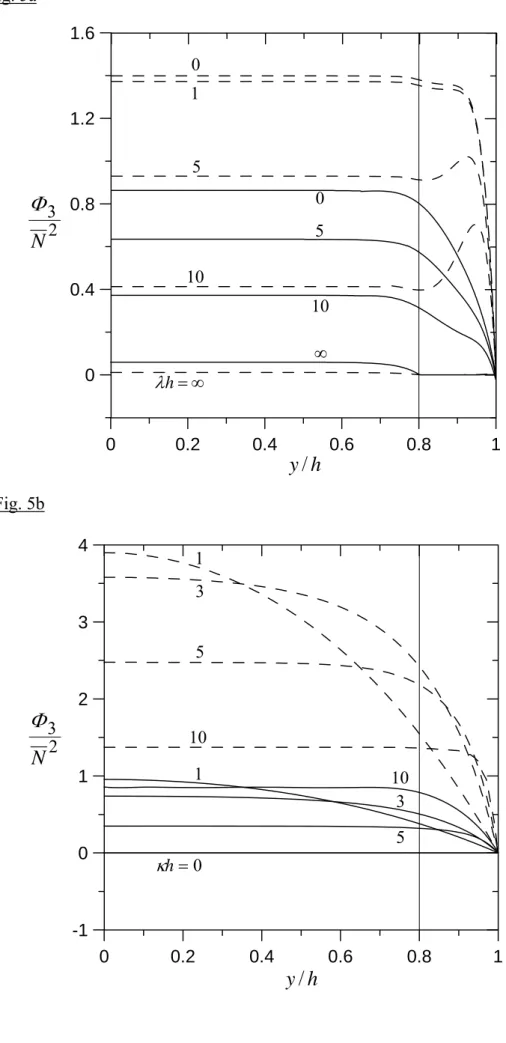
The functions Φ₁, Φ₂, and Φ₃ given by Eq. (27) for the general case and by Eqs. (31), (33), (35), and (37) for several special cases determine the diffusioosmotic velocity of a symmetric electrolyte in a capillary slit with each of its inside walls covered by a layer of adsorbed polyelectrolytes according to Eq. (26) correct to the second orders of σ (or ζ ) and N . Some graphical results concerning Φ₁/N and Φ₂/ N2 (and Zeψ /kTN) as functions

of the dimensionless coordinate can be found in the literature [21]. In Fig. 3, the function

h y /

2 3/ N

Φ for a slit filled with adsorbed polyelectrolytes (with ) calculated form Eq. (37) is plotted versus for several values of the parameters

0 /h= b

h

y / ζ /N, hκ , and hλ .

It can be seen that Φ₃ is positive, meaning that the effect of the lateral distribution of the induced axial electric field in the slit will cause the fluid flowing towards the end of higher electrolyte concentration. As expected, the value of Φ₃ is a monotonically decreasing function of y /h from a maximum at the median plane (with y=0) between the slit walls to

zero at the no-slip walls (with y=h). The value of Φ₃/ N2 in general increases with an increase in ζ /N . Evidently, Φ₃ increases with an increase in the value of hκ and

decreases with an increase in the value of hλ , for an otherwise specified condition. In the limiting situations that κh=0 (there is no interaction between the diffuse ions and the fixed charges) or λh→∞ (there is no flow penetration into the polymer layer), Φ₃ vanishes at any position in the capillary.

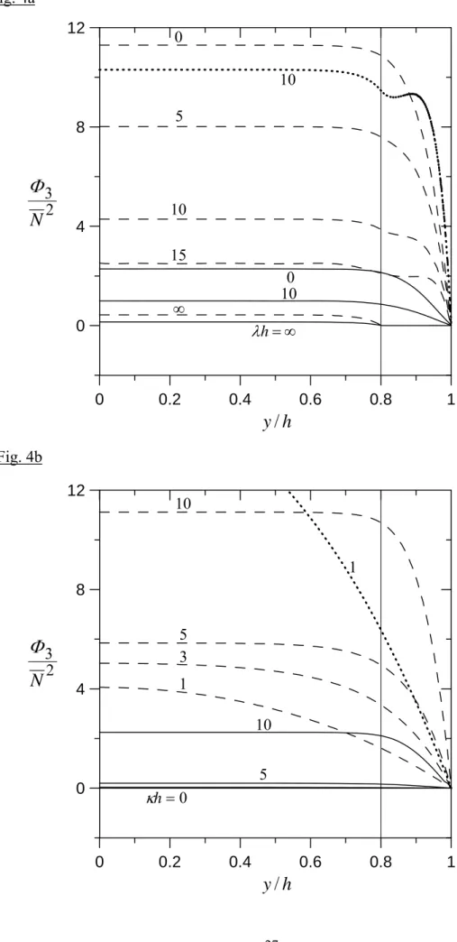
The function Φ₃/ N2 for a capillary slit with its inside walls covered by finite layers of adsorbed polyelectrolytes (with b/h=0.8 as an example) is plotted versus the relative position

in Figs. 4 and 5 for different values of the parameters

h

is positive for given values of these parameters, equals zero everywhere in the capillary for the limiting case of κh=0, and decreases with an increase in hλ for an otherwise fixed condition. When the magnitudes of ζ /N and hλ are relatively large, Φ₃/ N2 is not a monotonic

function of due to the existence of the finite polyelectrolyte layers on the slit walls. In the limit h y / ∞ → h

λ , Φ₃ vanishes within the surface charge layer ( ) as expected, but can be finite at other locations in the capillary. For the case of

b y>

0

/N ≥

ζ , as illustrated in Fig. 4, the value of Φ₃/ N2 increases with an increase in hκ or ζ /N for an otherwise specified

condition. For the case of ζ /N <0, as shown in Fig. 5, Φ₃ at a given relative position not

too close to the slit walls may not be a monotonically increasing function of hκ .

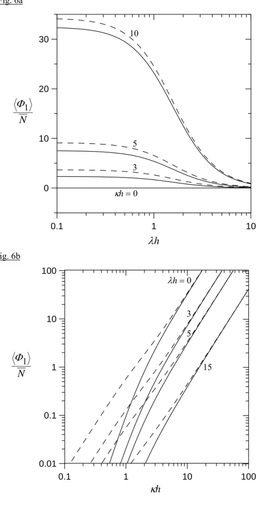
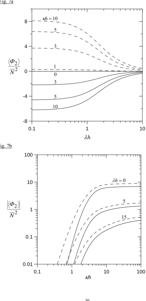
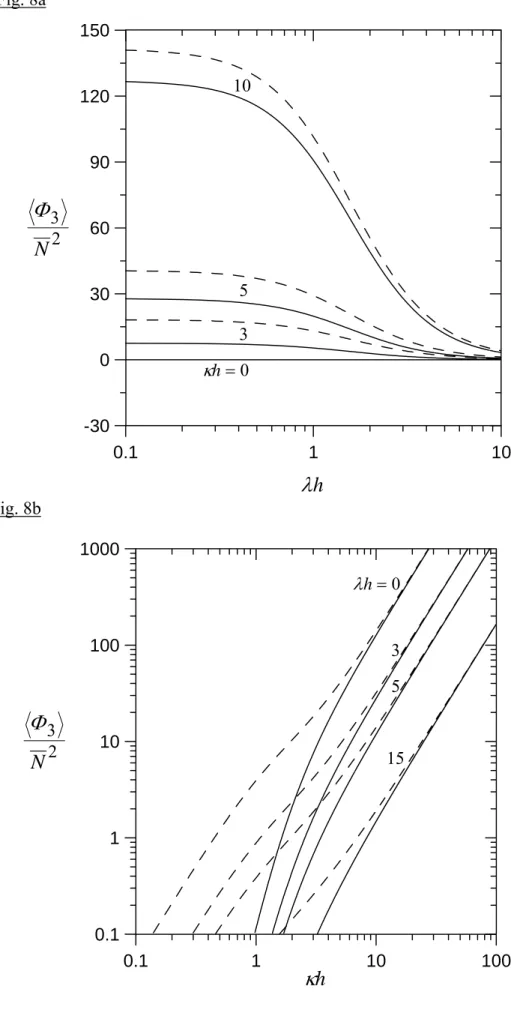
In Figs. 6, 7, and 8, the averaged values Φ₁ /N, Φ₂ / N2, and Φ₃ / N2, respectively, calculated from Eq. (38) as functions of the relevant parameters are plotted for a slit filled with adsorbed polyelectrolytes. For all cases, both Φ₁ /N and Φ₃ / N2 are positive, and the dependence of these values on the parameter ζ /N becomes relatively weak when the

magnitude of the parameter hκ is large. On the other hand, Φ₂ / N2 is positive as

1 /N >

ζ , negative as 0≤ζ /N <1, and vanishes as ζ /N =1. For the case of ζ /N <0

(which is not plotted here for conciseness), Φ₂ / N2 can be either positive or negative depending on the combination of ζ /N and hκ . As expected, the magnitudes of all these

three average functions increase with an increase in the value of hκ (the dependence for

2 2 / N

Φ is weaker than for the other two functions when hκ is large) and decrease with an increase in the value of hλ , for an otherwise specified condition. In the limiting situations that κh=0 or λh→∞, Φ₁ = Φ₂ = Φ₃ =0 and there is no fluid flow in the capillary.

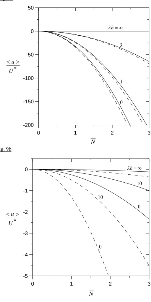
The dependence of the normalized average diffusioosmotic velocity u /U* of an electrolyte solution in a capillary slit with each of its inside walls covered by a layer of adsorbed polyelectrolytes on the dimensionless fixed-charge density N at a fixed value of hκ and various values of ζ /N, hλ , and b /h calculated from Eqs. (29) and (30) is displayed in Figs.

9 and 10. Because our analysis is based on the assumption of small electrostatic potentials, the magnitudes of N considered are less than 3. Fig. 9 is drawn for the case of a symmetric electrolyte that the cation and anion diffusivities are equal (β =0, representing the aqueous solution of KCl if Z =1). Only the results at positive values of N are shown because the

fluid velocity, which is due to O(ζ2,ζN, N2) contribution entirely as illustrated by Eqs. (29)

and (30), is now an even function of N . It can be seen from Eq. (29) and Figs. 7 and 8 that the fluid flows contributed from chemiosmosis (involving the function Φ₂) and electroosmosis (involving Φ₃) are in the same direction as 0≤ζ /N <1 but in the opposite directions as

1 /N >

ζ , and the net flow is dominated by the electroosmotic effect (having the direction of increasing electrolyte concentration). As expected, the magnitude of u /U* increases monotonically with an increase in N and with a decrease in hλ for constant values of

N

/

ζ , hκ , and b /h. There is no diffusioosmotic motion of the fluid for the special case of

0 = = N

ζ . In a previous study of the same diffusioosmosis [21], the

contribution from electroosmotic effect was not considered, and the resulted fluid velocity (which is due to chemiosmotic effect only) for the case of

) , , ( 2 N N2 O ζ ζ 1 /N >

ζ was in the direction of decreasing electrolyte concentration.

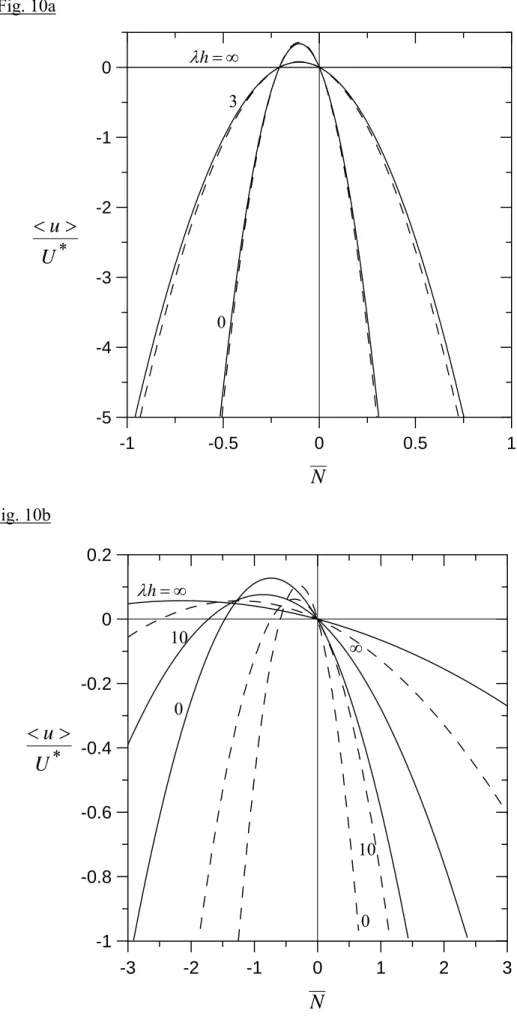
In Fig. 10, the normalized average diffusioosmotic velocity u /U* as a function of N is plotted for the case of a symmetric electrolyte whose cation and anion have different diffusion coefficients (β =−0.2 is chosen, representing the aqueous solution of NaCl if Z =1). In this

case, the diffusioosmotic velocity is neither an even nor an odd function of N . It can be seen that the fluid velocity is not necessarily a monotonic function of the magnitude of N for fixed values of ζ /N, hκ , hλ , and b /h. The curves in the vicinity of N =0 indicate that the fluid might reverse direction of flow more than once as N varies in a narrow range from negative to positive values. The reversals occurring at the values of N other than zero result from the combination of the contributions from electroosmosis of O( Nζ, ) and

) , ,

( 2 N N2

O ζ ζ (which is still dominant in many situations) and chemiosmosis of . Again, for specified values of

) , ,

( 2 N N2

O ζ ζ ζ , N , hκ , and b /h, the magnitude of

* /U

u decreases monotonically with an increase in hλ . In general, the net diffusioosmotic flow is still dominated by the electroosmotic contribution and in the direction of increasing electrolyte concentration.

6. Concluding remarks

The steady diffusioosmotic flow of solutions of symmetric electrolytes in a narrow capillary slit bearing a layer of adsorbed polyelectrolytes on each of its inside walls is analytically studied in this project. Solving the linearized Poisson-Boltzmann equation and the modified Navier-Stokes/Brinkman equation applicable to the system, the electrostatic potential distribution and the fluid velocity profile under the influence of a constant gradient of the electrolyte concentration are obtained in closed forms to the orders ( Nζ, ) and (ζ2,ζN,N2), respectively. The macroscopic electric field induced by the prescribed electrolyte concentration gradient through the capillary slit is a function of the lateral position rather than a constant bulk-phase quantity. The contribution to the diffusioosmotic flow made by the position dependence of the induced electric field is of the same order [ ] as, but may have an opposite direction to, that made by the chemiosmotic effect, and the former is dominant in most practical situations, as indicated by Eq. (26). Therefore, the effect of the deviation of the induced axial electric field in the slit from its bulk-phase quantity, which causes the fluid flowing towards the end of higher electrolyte concentration, can not be neglected in the evaluation of the diffusioosmotic flow rate in a capillary, even for the case of very thin double layer. Our results demonstrate that the structure of the surface charge layer can lead to a quite different diffusioosmotic flow from that in a capillary with bare walls [16], depending on the characteristics of the capillary, of the surface charge layer, and of the electrolyte solution.

) , ,

( 2 N N2 O ζ ζ

E

The macroscopic electric field arising spontaneously due to the imposed concentration gradient of the electrolyte in the axial direction of the capillary slit is provided by Eq. (15) or (19), and the diffusioosmotic velocity of the electrolyte solution is obtained in Eq. (26). In addition to the ionic fluxes due to electric migration (given by the second term in the brackets of Eq. (14)), the induced electric field can generate an electric current by electric conduction. Moreover, the diffusioosmotic fluid flow leads to another electric current by ionic convection. These two electric currents are not included in the current balance for the determination of . Thus, a secondary induced electric field must build up through the capillary, which is just sufficient to prevent the net electric current flow. This secondary electric field and its contribution to the fluid flow can be calculated via a similar approach in the calculations of the streaming potential induced across the capillary in the presence of an applied pressure gradient [2, 3, 20].

E

u

E

Appendix

For conciseness the definitions of some functions in Section 4 are listed here. In eq. (27), ] sinh ) ( [ ) ( ₂ 2 _{2 2} 10 x F x A x g − − = λ κ κ λ κ , (A1a) )] 2 2 (sinh ) ( 8 ) ( 4 4 [ ) ( ₂ 2 2 2 2 4 2 2 2 20 x F x NF x A x x g − − − + − = λ κ κ λ κ κ λ κ , (A1b) )] 2 2 (sinh ) ( 8 ) ( 4 4 [ ) ( ₂ 2 2 2 2 4 2 2 2 30 x F x NF x A x x g − + − + − = λ κ κ λ κ κ λ κ ; (A1c) , (A2a) x A x g₁₁( )= cosh ) 2 2 (cosh 2 1 ) ( 2 2 21 x A x x g = − , (A2b) ) 2 2 (cosh 2 1 ) ( 2 2 31 x A x x g = + ; (A2c) N x F x g 2 2 1 2 2 2 12( ) ( ) λ κ λ κ κ − − = , (A3a) ) 2 2 ( 2 ) ( 8 ) ( 4 2 ) ( 2 2 2 2 2 2 1 2 2 2 3 2 2 2 22 x F x NF x A B C N g + − + − − + − = λ κ λ κ κ λ κ κ , (A3b)

2 2 2 22 32(x) g (x) 4 A g λ κ − = , (A3c) where , (A4a) x C x B x F₁( )= cosh + sinh 2 x B x C x, (A4b) F ( )= sinh + cosh , (A4c) x BC x C B x F₃( )=( 2 + 2)cosh2 +2 sinh2 . (A4d) x BC x C B x F₄( )=( 2 + 2)sinh2 +2 cosh2 In Eq. (30), h x A x s κ sinh ) ( 11 = , (A5a) ) 4 2 sinh 3 ( 12 1 ) ( 2 3 21 A x x h x s = − κ , (A5b) ) 4 2 sinh 3 ( 12 1 ) ( 2 3 31 A x x h x s = + κ ; (A5c) ) ( )] ( ) ( [ 1 ) ( 2 2 2 2 2 2 12 N h x h x F h F h x s − − − − = κ λ κ κ λ κ κ κ , (A6a) )] ( ) ( [ 8 )] ( ) ( [ 4 1 ) ( ₂ 2 _{2 4 4 2} 2 _{2 2 2} 22 N F h F x h x F h F h x s − − + − − = κ λ κ κ κ κ λ κ κ κ ) )( 2 2 ( 2 _{2 2 2} 2 2 A B C N h x h − − + − + κ λ κ , (A6b) ) ( 4 ) ( ) ( _{22 2} 2 32 A h x h x s x s = − κ − λ κ . (A6c) In Eqs. (35) and (36), ) ( ) ( ) ( _{1 1} 13 x F h F x g = κ − , (A7a) ) ( 8 )] ( ) ( [ 2 1 ) ( ) ( _{33 3 3 13} 23 x g x F h F x Ng x g = = κ − + ; (A7b) )] ( ) ( ) )( ( [ 1 ) ( _{1 2 2} 13 F h h x F h F x h x s = κ κ − − κ + κ , (A8a) ) ( 8 )] ( ) ( [ 4 1 ) )( ( 2 1 ) ( ) ( _{33 3 4 4 13} 23 F h F x Ns x h x h h F h x s x s = = − − κ − + κ κ κ κ . (A8b) In Eqs. (37) and (38), N x B x g ₂ 2 1 2 2 2 14( ) cosh λ κ λ κ κ − − = , (A9a) ) 4 ( 2 cosh 8 2 cosh 4 2 ) ( ₁2 ₁ 2 2 1 2 2 2 2 1 2 2 2 24 x B x B N x B B N g + + − + − = λ κ λ κ κ λ κ κ , (A9b) 2 1 2 2 24 34(x) g (x) 4 (B N) g = − + λ κ ; (A9c) N h x h x B x s 2 1 2 2 2 14( ) sinh λ κ κ λ κ κ ₋ − = , (A10a)

) 4 ( 2 sinh 8 2 sinh 4 ) ( ₂2 _{2 1}2 ₂ 2 _{2 1 2 1}2 ₁ 24 B B N h x h x N B h x B x s + + − + − = λ κ κ λ κ κ κ λ κ κ , (A10b) 2 1 2 24 34( ) ( ) 4 (B N) h x x s x s = − + λ κ , (A10c)

and B₁ was defined by Eq. (13).

References

[1] M. Smoluchowski, in: I. Graetz (Ed.), Handbuch der Electrizitat und des Magnetismus, vol. II, Barth, Leipzig, 1921, p. 336.

[2] D. Burgreen, F.R. Nakache, J. Phys. Chem. 68 (1964) 1084. [3] C.L. Rice, R. Whitehead, J. Phys. Chem. 69 (1965) 4017.

[4] S.S. Dukhin, B.V. Derjaguin, in: E. Matijevic (Ed.), Surface and Colloid Science, vol. 7, Wiley, New York, 1974.

[5] J.L. Anderson, K. Idol, Chem. Eng. Commun. 38 (1985) 93.

[6] J.H. Masliyah, Electrokinetic Transport Phenomena, AOSTRA, Edmonton, Alberta, Canada, 1994.

[7] C. Yang, D. Li, J. Colloid Interface Sci. 194 (1997) 95.

[8] A. Szymczyk, B. Aoubiza, P. Fievet, J. Pagetti, J. Colloid Interface Sci. 216 (1999) 285. [9] D.C. Prieve, Adv. Colloid Interface Sci. 16 (1982) 321.

[10] D.C. Prieve, J.L. Anderson, J.P. Ebel, M.E. Lowell, J. Fluid Mech. 148 (1984) 247. [11] J.L. Anderson, Annu. Rev. Fluid Mech. 21 (1989) 61.

[12] H.J. Keh, S.B. Chen, Langmuir 9 (1993) 1142. [13] J.C. Fair, J.F. Osterle, J. Chem. Phys. 54 (1971) 3007.

[14] V. Sasidhar, E. Ruckenstein, J. Colloid Interface Sci. 85 (1982) 332.

[15] G.B. Westermann-Clark, J.L. Anderson, J. Electrochem. Soc. 130 (1983) 839. [16] H.J. Keh, H.C. Ma, Colloids Surfaces A 233 (2004) 87.

[18] H. Ohshima, T. Kondo, J. Colloid Interface Sci. 135 (1990) 443.

[19] V.M. Starov, Y.E. Solomentsev, J. Colloid Interface Sci. 158 (1993) 166. [20] H.J. Keh, J.M. Ding, J. Colloid Interface Sci. 263 (2003) 645.

[21] J.H. Wu, H.J. Keh, Colloids Surfaces A 212 (2003) 27. [22] K.A. Sharp, D.E. Brooks, Biophys. J. 47 (1985) 563.

[23] K. Morita, N. Muramatsu, H. Ohshima, T. Kondo, J. Colloid Interface Sci. 147 (1991) 457. [24] O. Aoyanagi, N. Muramatsu, H. Ohshima, T. Kondo, J. Colloid Interface Sci. 162 (1994)

222.

[25] A.W. Adamson, Physical Chemistry of Surfaces, 5th ed., Wiley, New York, 1990.

[26] V.G. Levich, Physicochemical Hydrodynamics, Prentice Hall, Englewood Cliffs, NJ, 1962.

Figure captions

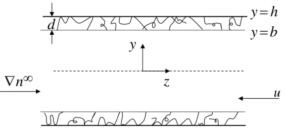
Fig. 1. Geometrical sketch for the diffusioosmosis in a capillary slit with each of its inside walls covered by a layer of adsorbed polyelectrolytes.

Fig. 2. Plots of the ratio σ/N for a capillary slit with its inside walls covered by layers of adsorbed polyelectrolytes versus the parameter hκ : (a) b/h=0; (b) b/h=0.8.

Fig. 3. Plots of the function Φ₃/ N2 for a capillary slit filled with adsorbed polyelectrolytes (b/h=0) versus the relative position y /h: (a) κh=10; (b) λh=1. The dashed, solid, and dotted curves represent the cases ζ /N =2, 0, and −2, respectively.

Fig. 4. Plots of the function Φ₃/ N2 for a capillary slit with its inside walls covered by layers of adsorbed polyelectrolytes versus the relative position y /h as b/h=0.8: (a) κh=10; (b)

1 = h

λ . The solid, dashed, and dotted curves represent the cases ζ /N =0, 2, and 4,

Fig. 5. Plots of the function Φ₃/ N2 for a capillary slit with its inside walls covered by layers of adsorbed polyelectrolytes versus the relative position y /h as b/h=0.8: (a) κh=10; (b)

1 = h

λ . The solid and dashed curves represent the cases ζ /N =−1 and −2, respectively.

Fig. 6. Plots of the function Φ₁ /N for a capillary slit filled with adsorbed polyelectrolytes (b/h=0) versus the parameters λh and hκ . The solid and dashed curves represent the cases ζ /N =0 and 2, respectively.

Fig. 7. Plots of the function Φ₂ / N2 for a capillary slit filled with adsorbed polyelectrolytes (b/h=0) versus the parameters λh and hκ . The solid and dashed curves represent the cases ζ /N =0 and 2, respectively.

Fig. 8. Plots of the function Φ₃ / N2 for a capillary slit filled with adsorbed polyelectrolytes (b/h=0) versus the parameters λh and hκ . The solid and dashed curves represent the cases ζ /N =0 and 2, respectively.

Fig. 9. Plots of the normalized average diffusioosmotic velocity u /U* in a capillary slit with its inside walls covered by layers of adsorbed polyelectrolytes versus the dimensionless charge density N with κh=10 and β =0: (a)b/h=0; (b)b/h=0.8. The solid and dashed curves represent the cases ζ /N =0 and 2, respectively.

Fig. 10. Plots of the normalized average diffusioosmotic velocity u /U* in a capillary slit with its inside walls covered by layers of adsorbed polyelectrolytes versus the dimensionless charge density N with κh=10 and β =−0.2: (a)b/h=0; (b)b/h=0.8. The solid and dashed curves represent the cases ζ /N =0 and 2, respectively.

Fig. 1

d

u

h

y

=

b

y

=

y

∞

∇

n

z

Fig. 2a 0 1 2 3 4 5 -3 -2 -1 0 1 2 2 /

N

N

h

κ

N

N

h

κ

Fig. 3a 0 0.2 0.4 0.6 0.8 1 0 50 150 200 ₀ 1 2 3

N

Φ

h

y

/

N

Φ

h

y

/

Fig. 4a 0 0.2 0.4 0.6 0.8 1 0 4 8 12 ₀ 10 5 0 0.2 0.4 0.6 0.8 1 0 4 8 12 Fig. 4b 0 = h κ 3 5 10 1 10 5 ∞ = h λ 10 ∞ 10 15 0

h

y

/

h

y

/

N

Φ

N

Φ

Fig. 5a 0 0.2 0.4 0.6 0.8 1 -1 0 1 2 3 4 0 0.2 0.4 0.6 0.8 1 0 0.4 0.8 1.2 1.6 0 1 5 0 2 3

N

Φ

y h

/

N

Φ

h

y

/

Fig. 6a 0.1 1 10 0 10 20 30 10

N

Φ

h

λ

N

Φ

h

κ

Fig. 7a 0.1 1 10 100 0.01 0.1 1 10 100 0.1 1 10 -8 -4 0 4 8 κh=10 5 3 2 2

N

Φ

h

λ

N

Φ

h

κ

Fig. 8a 0.1 1 10 -30 0 30 60 90 120 150 10 2 3

N

Φ

h

λ

N

Φ

h

κ

Fig. 9a 0 1 2 3 -200 -150 -100 -50 0 50 ∞ = h λ 3 *

U

u

>

<

N

U

u

>

<

N

Fig. 10a -1 -0.5 0 0.5 1 ∞ = h λ -5 -4 -3 -2 -1 0 3 *

U

u

>

<

N

U

u

>

<

N

（一）參加會議經過

「 澳 洲 膠 體 與 界 面 研 討 會 」 (Australian Colloid and

Interface Symposium)是由澳洲膠體與界面學會(ACIS)主辦，近

年來每兩年舉行一次，是國際間膠體與界面科學相關領域之重

要學術會議。今（2007）年的會議是第三屆，依往例在澳洲雪

梨東方的 Coogee 海灘假日旅館 Crowne Plaza Hotel 會議廳舉

行，會期從二月四日至八日共計五天。

此 次 會 議 共 有 二 百 餘 篇 論 文 發 表 ， 其 中 plenary and

keynote lectures 十六篇，一般論文中口頭發表 (lectures) 部份

計有一百餘篇，分別安排於五天會期中；另外有一組全天的海

報展示（posters）時段。會議期間主要活動除了論文發表與討

論外，還包括書籍與期刊展示、以及海灘參觀活動。此次參加

會議的學者專家超過二百人，分別來自澳洲及其他約十六個國

家。較著名的學者包括德國的 W. Knoll， 英國的 B. Vincent，

美國的 J. N. Israelachvili, D. L. Sparks, G. E. Brown 與 D.

Wasan，以及荷蘭的 U. Schubert，他們並分別就其專長領域各

做了二十至六十分鐘的專題演講，內容頗為豐富。

筆者此次發表的研究論文「液滴垂直二平板之熱毛細運

動」（Thermocapillary migration of a fluid drop perpendicular to

two plane walls）被安排在會議正式議程第一天（二月五日）的

海報展示時段中作一整天展示，並於下午 18:00-20:00 二小時

中接受與會者之詢問與討論。在休息的時間中，亦有不少與會

人士與筆者繼續就此篇論文的內容交換意見，氣氛熱烈融洽。

（二）與會心得

此次會議，筆者除了發表一篇論文外，亦積極參與議程

中之聽講與討論，並參觀海報論文展示，頗有獲益良多之感。

筆者對於有關膠體輸送現象以及界面電動力現象的三十幾篇論

文最感興趣，發現國際間此領域的研究有以下幾個新的發展趨

勢：

（1）對於膠體粒子輸送現象之相關研究，已從過去的球形

粒子，剛性粒子，單一或兩、三個粒子，以及無孔隙粒子的單

純情形，延伸到非球形粒子，非剛性粒子，多個粒子，以及多

孔隙粒子等較複雜的情況。

（2）對於膠體粒子表面電雙層（electric double layer）的分

析，已從過去理想的均勻分佈，平衡狀態及無濃度極化現象，

延伸到非均勻分佈，非平衡狀態以及有濃度極化現象等較實際

的情況。

（3）對於固體表面的處理，已從過去的平滑表面、無吸附

情況、以及均勻表面電位（zeta potential）分佈的單純情形，延

伸到粗糙表面、表面吸附高分子物質、以及非均勻表面電位分

佈等較複雜的情況。

（4) 逐漸研究帶電多孔物質 (如薄膜、膠體粒子凝聚體)

中之微小粒子或電解質溶液的輸送現象。

（5) 進行高濃度膠體懸浮液之電動力性質（如粒子表面電

位、電泳、沉降電位、電導度、介電行為等）的理論分析與實

驗量測。

（三）建議

(1) 國內目前之研究環境及經濟條件，對發展中國家的研

究人員而言，相當具有吸引力。可考慮邀請具有學術地位的學

者及研究潛力的博士後研究員來台短期訪問或長期研究，以增

強我國的學術水準。

（2）一般學術性的研討會大多以學術性與基礎研究性的

論文題目較受與會者重視，國科會應多鼓勵國內研究人員從事

學術性與基礎性的研究。

（3）政府應鼓勵國內優秀的研究人員多參加有水準的專

業性國際學術會議發表論文，藉以吸收國際間最新的研究成果

與方向，並提昇國內研究表現在國際學術界的能見度與地位。

（四）攜回資料

「ACIS 2007澳洲膠體與界面研討會」之會議論文摘要集

一冊。