行政院國家科學委員會專題研究計畫 期中進度報告
蛋白質立體結構預測(2/3)
計畫類別: 個別型計畫 計畫編號: NSC92-3112-B-002-001- 執行期間: 92 年 05 月 01 日至 93 年 04 月 30 日 執行單位: 國立臺灣大學資訊工程學系暨研究所 計畫主持人: 高成炎 共同主持人: 楊進木 報告類型: 完整報告 報告附件: 出席國際會議研究心得報告及發表論文 處理方式: 本計畫可公開查詢中 華 民 國 93 年 3 月 2 日
關鍵詞(keywords): Human genome project, Family Competition Evolution Algorithm, Rotamer Library, Lattice Model, ab initio, Tertiary protein structure, Secondary Structure Prediction, HP model, Support Vector Machine, Disulfide-bond connectivity
一、 中文摘要:
自然界生物有機體的蛋白質結構 (Protein structure) 都被賦予幫助生存的特別功能,這些 蛋白質會因為不同形狀的3D 立體結構 (three- dimensional structures) 而有特別的功能及負責的 任務,因此,3D 立體結構將決定蛋白質的功能及作用。而 3D 結構是由 1D 結構,也就是蛋白 質氨基酸序列所組成的鍊狀物,由線性的形狀透過本身機制折疊(fold)成 3D 結構,折疊的機制 是目前許多研究者研究的方向,希望能夠瞭解為什麼可以蛋白質在短短的幾毫秒時間能夠形成 立體結構的原因。 蛋白質結構折疊的問題在計算分子生物學裡頭是一個非常重要且有名的難題。即使簡化 成HP 模型,在計算理論上亦是 NP-Hard 的問題,平常的演算法無法在短時間內得到好的結果。
我們嘗試以家族競爭式演化方法 (Family Competition Evolutionary Algorithms) 從蛋白質序列的 觀點,來預測蛋白質的立體結構,此演算法的目的是專門解決最佳化問題。我們設計以立體晶 格模型 (Lattice model) 顯示蛋白質結構,並使用氨基酸各種不同的特性來表示晶格上的氨基 酸。
本計畫中,我們在晶格模型中可以輸入氨基酸序列,家族競爭式演化方法將透過重組操 做 (Recombination Operator) 及突變運算 (Mutation Operator) 產生不同的子代,我們將進行關 於凝聚函數、殘基間相互影響的能量函數及親水疏水能量的計算,每個所產生的結構都將被運 算,根據運算的結果,我們將取得能量最低且穩定的結構作為我們預測的結果,經過幾代的演 進之後,最後得到穩定的結果,這即是最佳的立體結構。使用者可以透過我們以圖形視覺化介 面的工具看到整個折疊模擬的過程,也可以視需要調整觀看的結構角度,最後將顯示出最穩定 的結構。除了使用晶格模型之外,本計劃使用各種不同的機器學習技術,由蛋白質序列中預測 結構上的特徵,例如二級結構,雙硫鍵樣式等等。最後匯整所有的資訊,用立體結構模擬的方 法,加上快速能量計算晶片的幫助,預測蛋白質的結構。 本系統使用演化式演算法來找出最佳化的結構,再配合設計的操作,能量評估等化學特 性,希望能解決組合性爆炸的問題,找出最佳解供從事蛋白質結構研究的研究員一些幫助,也 可以加速及減少實驗上的成本,讓研究員可以在 X 光晶體繞射 (x-ray) 或核磁共振 (nuclear magnetic resonance ,NMR) 得到立體結構的方式外,多了一項選擇。
二、 英文摘要:
Protein functions are decided by their three-dimension structure. We have explored the application of family competition evolutionary algorithms (FCEA) to the determination of protein structure from sequence. The algorithm is proposed to solve optimization problem. The protein structures are showed with a square lattice of we design. The protein component uses Hydrophobic-hydrophilic model (HP model) to calculate structure energy. The protein components are reduced to a binary class: P for polar, hydrophilic monomers, and H for non-polar, hydrophobic monomers.
We can input amino acid sequence or HP sequence to lattice model in our system. The operation of recombination and mutation of FCEA will produce many different offspring. We will calculate structure energy that are distance function, residues-residues interaction function and HP function on every three-dimension structure of lattice model. According to the calculated result, the system will select the lowest energy. After many generations, the result will be stable status and optimization structure. The user can see the process that folding simulations and adjust the structure angle in our visual tool. The last stable structure will be show in the monitor.
三、 前言:
生物體是倚靠體內蛋白質的運作來維繫生命現象,目前對於自然界如何從蛋白序列轉變成 立體結構的過程並不瞭解,因此,便有一些研究學者設計各種實驗方法,試圖瞭解蛋白質形成 立體結構的過程,想藉著這些方法來進行蛋白質立體結構的預測。 蛋白質結構預測已經研究超過30 年,想要藉由一些實驗來瞭解蛋白質所形成的三維立體 結構,成本高又耗時。解一個蛋白質結構往往需要很長的時間,先前IBM 的超級電腦 (Super Computer) 模擬一個小的蛋白質結構也需要一年的時間,所以準確的蛋白質結構預測是十分困 難的工作,需要考量很多因素。 有一些預測結構的方法是從蛋白質序列出發,運用一些技術來作預測立體結構。以前的 實驗中,蛋白質序列通常已經折疊的結構中所取得[5,6],然而當時的實驗都是以小型蛋白質切 成多個小片段來取得資料,再組合這些資訊做出完整的結構,蛋白質折疊的方法便成為蛋白質 形成立體結構的關鍵[21,35],原則上,這些計算都需要靠功能強大的電腦的幫助,在折疊模擬 的過程中挑出幾個可能的結構作為預測的結果,至於預測的結果好不好,則分別計算這些結構 的能量,以能量最穩定的結構作為最後選擇的答案[2,8],為了節省計算的時間,有些研究人員 簡化了計算能量的函數及 3D 空間所帶來的複雜度,希望能解決這個關於複雜計算量的問題 [19,22,23,36], 後來便有人提出以晶格(Lattice) 的表示法來表示立體結構中每一個氨基酸的位 置[12,14,20],及精確的描繪出蛋白質主鍊結構預測的設計方法[11,27,28]。 基於這樣的想法,我們運用由基因演算法 (Genetic Algorithm) 所發展出的家族競爭式演 算 法 (family competition evolutionary approach algorithm) , 再 加 上 親 水 疏 水 性 的 模 型 (Hydrophobic -hydrophilic model) 來進行蛋白質折疊模擬 (Protein Folding Simulation) ,希望結 合目前科技,試著以先進的電腦軟硬體技術輔助,來模擬蛋白質由序列轉變成立體結構的過 程,並以最少時間及成本預測出蛋白質三維立體結構。目前有許多研究機構投入蛋白質結構預測 (Protein structure prediction) 的工作,每個機構 都採用不同的方法加以研究,有些單位是結合蛋白質二級結構 (Protein secondary structure) 的
資訊;有些使用Lattice 模型來表示蛋白質結構;有些固定蛋白質主鍊 (backbone),使用支鍊
(side-chain) 的資訊等,選擇操作模型後,最後再以演算法來解決組合性爆炸的問題,這些演 算法包含蒙地卡羅 (Monte Carlo) 隨機法、遺傳演算法 (Genetic Algorithm) 及動態規劃 (Dynamic programming) 等來進行預測,其中的 Lattice 模型即是本篇所使用的方法。
除了 Lattice Model 之外,一些從蛋白質序列中萃取出來的資訊,例如二級結構,支鍊的 構型,雙硫鍵的連接樣式等等。也會加入最後立體結構的模擬,提高整體的準確性。本計劃還 開發了專門計算分子等級的能量 (Amber Function) 晶片,藉由硬體的加速,縮短預測蛋白質 結構的時間。
四、 研究目的:
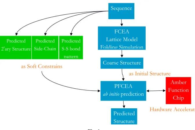
A reliable prediction and precise classification of proteins structure and function of has become increasingly important due to the completion of Human Genome project and other genome projects. The Protein folding problems is one of the most computation extensive tasks the scientific community facing these days. In the past few years, our group has developed an efficient evolutionary algorithm, Family Competition Evolution Algorithm (FCEA), to solve problems in Structure-Base Drug Design, Protein Side-Chain Prediction, and other optimization problems. The performance of the algorithm is very promising. It is a very powerful stochastic global optimization tool to search large sample space. In this project, we plan to extend our FCEA to parallel and distributed version and apply it to solve the Protein Folding Problem, as well as to investigate the following three prediction tasks about proteins from protein amino acid sequences:
1. Learning a model of protein folding
2. Predict protein structure features (Secondary Structure, Disulfide-pattern, Side-chain conformation) as soft constrains using machine learning skills
3. Designing an efficient distributed evolutionary algorithm (PFCEA) for the protein folding problem using PC-Cluster and ab initio method.
Fig. 1
FCEA
Lattice Model
Folding Simulation
Sequence
Predicted 2’ary StructureCoarse Structure
PFCEA
ab initio prediction
Predicted
Structure
as Soft Constrains
as Initial Structure
Predicted Side-Chain Predicted S-S bond patternAmber
Function
Chip
Hardware Accelerate
五、 文獻探討:
5.1 生物學與蛋白質 Biology and Protein
蛋白質是維持生物體的生理機制及各種催化的重要元素,大多的生命現象與新陳代謝 都是仰賴有功能的蛋白質,所以蛋白質是使得細胞內各項活動得以順利進行的主要關鍵。 蛋白質是由氨基酸連接而成,其結構可以分一級到四級結構 (圖一) 。
自然界中蛋白質氨基酸序列由線性形成立體結構的過程稱為蛋白質折疊 (Protein folding),這個結構是因為氨基酸間經由轉動或移動,也就是多肽鏈 (polypeptide chain) 折 疊或聚合之後,最後形成穩定的鍵結。蛋白質折疊的過程所需的時間大約是幾毫秒(μs) 至幾微秒 (ms) 之間,如此短暫的時間便可以完成結構,而其中的折疊過程目前還在持續 的研究中。
圖一:蛋白質結構 5.2 晶格模型與親水疏水模型 Lattice model and H-P model
本研究使用親水—疏水模型 (Hydrophobic-Hydrophilic Model) 簡稱 H-P 模型,這是由許 多晶格(cube)所屬組成,每一個晶格為立方體,立方體上的點代表的是蛋白質序列中該位置
為 20 種氨基酸(Amino acids)的哪一種,H-P 模型將這些氨基酸分成兩種型態,一種是疏水性
(hydrophobic),簡稱為 H,大多存在立體結構的內部;另外一種為親水性 (hydrophilic) 或是帶 極性 ( polar),簡稱為 P,大多存在於結構的表面 (protein surface),常與水溶液接觸,被水中
的帶電離子吸引。如圖一所示,黑點代表的是H,白點代表的是 P,蛋白質的立體結構便可由
圖二:H-P 模型 5.3 演化式計算 Evolutionary Computation
在解最佳化的問題時,往往會採用演化式演算法來計算,常見的算法包含動態環境學習 的分類式系統(Classifier system)、數值分析為主的演算法策略(Evolution Strategy)、人工智慧演 算 式 規 劃(Evolutionary Programming) 、 家 族 競 爭 方 式 的 演 化 式 方 法 (Family Competition Evolutionary Approach)、遺傳演算法(Genetic algorithm)、人工智慧型的遺傳規劃(Genetic programming)。
由人工智慧 (Artificial Intelligence,簡稱 AI) 研究領域所發展出來的運用生物演化方式的一 項學科—演化式計算 (Evolutionary Computation,簡稱 EC) ,可以快速的找到最佳解,其原理 是來自生物學家達爾文(Darwin)提出的「物競天擇,適者生存」的演化論,目前依照自然界生 物演化的機制,這樣的構想發展出幾套演算法。 目前生存在地球上生物體系的生物群體 (population) 中的個體 (individual) 在有限資源的環 境下,必須為了生存 (survival) 而競爭 (competition)。在達爾文的理論架構下,只有強者或稱 勝利者有生存下去的機會,也會經由繁衍後代來維繫生物型態的維繫,而失敗者將在被各種條 件篩選之下被淘汰出局,勝利者將透過生物的各種遺傳(genetic) 機制繁衍後代,這樣的子代 與父代有一定的相似度,也有可能因為較大的差異而產生新的物種,因此,在這樣的機制下所 產生的後代將演化成越來越能適應環境,每一個世代 (generation) 的調整也有助於適應當前的 生存環境。 根據上述的演化機制,所發展的各類演化式計算方法程序大致如下 (如圖四): 1.選擇及設定初值 (initialization) 群體。 2.評估 (evaluation) 群體中的個體,決定結束程序的條件。
3.對於群體中的個體依據適合度 (fitness function) 做選擇 (selection),評估中適存度較高的個 體較易生存,淘汰部份個體。
4.以突變(mutation)、交換(crossover)、複製(reproduction) 等遺傳運算 (genetic operation),產生 多個新的變異個體加入群體,而得到下一代的群體。
圖四:EC 一般的方式
針對各種問題不同的特性來設計方法,以最適當的方式設計不同的行為模式、個體結構、和 群體組織,以期待能更快速地解決問題。
5.4 家族競爭式演算法 Family Competition Evolutionary Approach
何謂家族競爭演化式,在最佳化問題中最難的是解決全域性最佳化(Global optimization) 的問題,家族競爭演化式(Family Competition Evolutionary Algorithm),簡稱 FCEA,此方法以 家 族 競 爭 (family competition) 及 適 應 規 則 (adaptive rule) 為 基 礎 , 並 整 合 遞 減 式 (decreasing-base) 及自我調整 (self-adaptive) 的突變 (mutation),使 FCEA 能同時具有區域性 最佳化及全域性最佳化兩者之長處的搜尋策略。我們將這一些策略結合之後,便具有全域性問 題最佳化的解決能力,並在較短的時間內得到好的結果。 FCEA 是一個可以解決全域性最佳化問題的演算法,它整合多個突變的運算,這套演算 法是由交通大學生命科學系楊進木教授於台灣大學資訊工程研究就所讀博士班時所發展出來 的。FCEA 的執行,根據初值隨機產生 N 個解答,接著進入主要競爭的循環,意圖找出最佳 解,每一代均會經過三次的處理,每一次的處理包含重新組合 (recombination) ,突變
(mutation),家族競爭 (family competition) 及最後的選擇。
何謂家族競爭(family competition)?簡單的說就是在同父異母的兄弟姊妹中,只有一個能
存活下來的淘汰法則。家族競爭的處理方式如圖六,一共有L 個子代被作重組及突變的運算,
而最後經過選擇後,只有最佳解會存在,其他的解將在競爭之下淘汰,如同達爾文的適者生存 的理論般。
圖五:家族競爭的步驟
每一個獨立的染色體 (In),我們稱為這一個家族的父代,這個父代配合產生的機率 Pc 隨機 產生一群解(I11...I1l),對於這一些解在組合後新結果,這些產生的子代(I11...I1l)及原來的家族 父代再經由突變後,選出最佳解(C1_best)。
我們定義經由FCEA 處理的資料稱做染色體(chromosome representation),染色體的資料格
式為由使用者訂定,如果染色體序列有 n 個長度,則資料由 X1...Xn。接著重組操做
(recombination operator),FCEA 有兩種簡單的重組運算,一種是修正式離散的重組方式,以固 定的比例重組。另外必須訂定不同的突變運算(mutation operator),產生不同的子代,突變的方 式有三種,分別是以遞減為基礎的高斯突變 (decreasing-based Gaussian mutation)、高斯自我適 應 突 變 (self-adaptive Gaussian mutation) 及 歌 西 自 我 適 應 突 變 (self-adaptive Cauchy mutation) , 最 後 還 有 依 照 不 同 的 評 估 方 式 所 規 範 的 兩 種 適 應 規 則 , 一 是 遞 減 規 則 (A-decrease-rule),如果父代評估結果優於子代中最好的一個,則選擇父代,並將突變率降低, 使得內容不至於變的太快,另外一個是遞增規則 (D-increase-rule),如果父代評估結果比子代 的差,則在最好的子代與平均的父代中選擇較佳的,成為下一個高斯自我適應突變參數,不斷 產生子代進行演化,最後趨於穩定則此即為最佳解的答案。
六、 研究方法與討論:
In this project, we will predict protein structure solely from amino-acid sequence using an ab initio method. It will involve three major steps – (1) adapt the HP model on a lattice system to gain a coarse structure; (2) predict secondary structure elements, and use the results as soft constraints to optimize an AMBER-like energy function and (3) place the side-chains with side-chain prediction results, and refine the structure.
We have the following progresses in the second year- 1. Lattice Model simulation
2. Predict the secondary structure by SVM 3. Predict Disulfide-Bond pattern by SVM 4. Amber function chip Implementation
1. Construct Lattice Model for folding simulation
The first step of our methodology was to simulate the protein structure on a lattice model, and minimize the hydrophobic energy to gain the coarse structure .We adapted the HP model to the contact energy function, and optimize the total energy of the system by our new Family Competition Evolutionary Algorithm (FCEA).
We considered the problem of determining the three-dimensional folding of a protein, given its one-dimensional amino acid sequence. The model we used was based on the Hydrophobic-Polar (HP) model (Dill 1985) on cubic lattices, in which the goal was to find the fold with the maximum number of contacts between non-covalently linked hydrophobic amino acids. Hart and Istrail (1995) gave a 3/8 approximation algorithm for folding proteins on the cubic lattice. Since the cubic lattice exhibits the ``parity'' problem (described below), we instead considered folding proteins on a different lattice: the three-dimensional triangular lattice. For this lattice, Decatur and Batzoglou (1996) gave a simple linear time algorithm which achieved a 16/30 asymptotic approximation. In this study, we further improved the model by generalizing the HP model to account for hydrophobic residues with different levels of hydrophobicity. After describing the motivation for this generalization of the model, we showed that in the new model we were able to achieve the same constant factor approximation guaranteed on the triangular lattice as was achieved in the standard HP model.
For the lattice model system, the space in which the protein folds discretized by defining a lattice and requiring residues to lie only on lattice points. Residues which were adjacent in the primary sequence (i.e. covalently linked) have always been placed at adjacent points in the lattice. A fold of a protein was simply a self-avoiding walk along the lattice. In order to distinguish the quality of a given fold of a protein, we showed that a contact between two residues was a topological contact if they were not covalently linked and there would be an edge connecting the lattice points of the two residues.
The original HP model abstracted the problem by classify the 20 amino acids which composed proteins into two classes: hydrophobic (or non-polar) residues and hydrophilic (or polar) residues. Then the free energy of a fold was defined to be (–1) x (# of topological contacts between pairs of hydrophobic residues). We often referred to the score of a fold as defined to be the absolute value of its free energy. The target fold for the protein is the one which has the lowest free energy, or equivalently, the highest possible score.
The biological foundation of this model is the belief that the first-order driving force of protein folding is due to a “hydrophobic collapse” in which those residues which prefer to be shielded from water (hydrophobic residues) are driven to the core of the protein, while those which interact more favorably with water (polar residues) remain on the outside of the protein. The protein is hypothesized to fold in such a way as to minimize the surface area of hydrophobic residues exposed to water or polar residues. The HP model has been studied extensively [Dill et.al, ].
Fig. 2
Table 1 shows the simulation results of our FCEA-based hydrophobic - hydrophilic model and other methods. The model optimized by FCEA obtains better HP scores than optimized by Monte
Carlo method [Ramakrishnan et al., 2003] or New Monte Carlo method [Bastolla et al., 2003] in three testing proteins. Fig. 3 shows the structure of testing proteins folded by our model.
Protein Length HP score (FCEA)
HP score (Monte Carlo)
HP score (New Monte Carlo)
Hp60 60 -44 -34 -36
Hp1001 100 -55 -44 -47
Hp1002 100 -52 -46 -49
Table 1
Hp60 hp1001 hp1002
Generation:115 Generation:601 Generation:258
HP score:-44 HP score:-59 HP score:-52
Fig. 3
2. Predict secondary structure by SVM
In this project, we exploit the possibility of using SVM for protein secondary structure prediction. We worked on similar data and encoding scheme as those in Rost and Sander. The results indicated that SVM easily returns comparable results as neural networks. Therefore, in the future, it is a promising direction to study other more recent neural-network-based approaches by using SVM.
Given an amino acid sequence, for each amino acid, we predicted it as an alpha helices, a beta strand, or a coil. The secondary structure assignment was done according to the DSSP algorithm, which distinguishes eight secondary structure classes. We converted the eight types into three classes in the following way: H (alpha-helix), I (pi-helix) and G (310-helix) were classified as helix (alpha), E (extended strand) as beta-strand (beta), and all others as coil (c).
. The encoding method we used in our study is basic on the evolutionary information. This method considered a moving window of 17 (typically 13-21) neighboring residues and representing each window using profile obtained from multiple alignments taken from the HSSP database. Prediction was made for the central residue in the windows. In this encoding scheme, for each residue the frequency of occurrence of each of the 20 amino acids at one position in the alignment is computed. In order to allow the moving window to overlap the amino- or carboxyl- terminal end of the protein, a null input was added for each residue. Therefore, each data consists of 17 windows and each window contains 21 attributes, where most of them have the value zero. The training data
consists of 24,387 records in three classes where 47% are coil, 32% are helix, and 21% are strand. Each record contains 21x17 = 357 attributes.
We evaluated the prediction system with seven-fold cross validation on a dataset used by Rost and Sander. The accuracy was 70.5% which is competitive with the results by Rost and Sander. We have to emphasize here again that we use the same data set and secondary structure definition. It has been shown by many researchers that using more data improve the prediction accuracy. The improvement may be due to the accidental addition of more easily predicted sequence to the set or better predictive patterns learned by the classifiers trained on more sequences. We have a similar observation while using SVM.
3. Predict Disulfide-bond pattern by SVM
While a protein folds into its native structure, two cysteine residues can be oxidized to form a disulfide bond. This covalent bonding is commonly found in extra-cellular proteins, which helps stabilizing the native conformation due to their contribution of thermodynamic stability in three-dimensional structure. Two cysteines are very close in 3D space if they form a disulfide bond. This kind of information will dramatically reduce the search space and raise the accuracy when we predict structures of proteins.
Several studies were investigated to predict disulfide-bonds. For examples, several classifiers were developed to predict the oxidation state of each cysteine residue from sequences by using neural networks, support vector machine, or HMM. The accuracy is about 70~80% which depend on the evolutionary information is considered or not. However, even the oxidation state of each cysteine residue is known, locations of disulfide bonds (i.e. disulfide connectivity pattern) are still difficult to determine. Farselli and Casadio transferred the disulfide-connectivity problem into an undirected graph, where vertices represent bonded cysteine residues and weights of edges are the binding potentials for corresponding cysteines. The connectivity pattern prediction was then turned into a problem of finding the maximum weight perfect matching. They trained the matrix of contact potential by simulated annealing (SA). Vullo and Frasconi trained a recursive neural network to score candidate graphs, and exhaustively search for the best scored graph to obtain the disulfide connectivity pattern.
In this paper, we predict the disulfide connectivity patterns with the information of bonded cysteines. A support vector machine (SVM) is applied to predict the bonded potential. After the potentials are generated, Edmonds’ algorithm is employed to find the disulfide connectivity patterns in proteins. In addition to the conventional sequence sliding window feature, the effect of predicted secondary structure, hydrophobicity, and sequential distance are explored.
The rest of this paper is organized as follows. Section 2 introduces the proposed approach. Data preparations are detailed in Section 3. Section 4 discusses the performance and important features. Concluding comments are drawn in Section 5.
There are two main steps in predicting the disulfide connectivity pattern: 1) estimating the probability (bonding potential) of each pair of cysteines forming a disulfide bond; and 2) predicting a disulfide connectivity pattern of a target protein according to the bonding potential. Therefore the proposed approach is composed of two mechanisms: 1) training a model to predict the bond potential for all pairs of cysteines from the training set; 2) for a sequence of protein, the predicted
bond potential is adopted to find the most possible disulfide connectivity pattern.
In this paper we observe disulfide bonded and non-bonded cysteines to estimate the bonding potential of each pair of cysteines forming a disulfide bond. Given a set of proteins with known structures, disulfide bonded and non-bonded cysteines are separated into positive and negative instances, respectively. For each instance, various features are collected to capture useful information of the pair of cysteines that can discriminate bonding pairs from non-bonding ones. These feature vectors of both positive and negative instances are used as the input to a classification tool to learn a classifier. In our approach, support vector machines (SVMs) is adopt as the classification tool. SVM is a new rising classification tool and becomes more and more popular. The support vector learning algorithm can avoid both under-fitting and over-fitting and hence reduce training and testing error. The concepts of training procedure are as follows.
Step 1: For each protein in the training set, collect all pairs of cysteines in bonding state, whether the pairs would form a disulfide bond or not, and extract necessary features from the sequence. Each instance is composed of one cysteine pair.
Step 2: Cysteine pairs of which form disulfide bonds as positive class, and others as negative class. Step 3: Use these instances as input of SVM and learn a classifier C. This classifier can predict a
probability whether a cysteine pair would form a disulfide bond.
Given a sequence with unknown structure where the bonding state of the cysteine residue is know, the resulting classifier predicts the probability of whether the pairs of cysteines of the sequence is disulfide bonded or not based on their feature vectors. A weighted complete graph is constructed in which vertices represents the cysteines, and the weight of edge between its two incident vertices is the bonding probability predicted by the classifier. According to this matching, a disulfide connectivity pattern is obtained. In finding maximal weight perfect matching in a graph, we used the algorithm proposed by Edmond and Johnson. The concepts of predicting procedure are as follows. Step1: Given a protein sequence, all pairs of cysteines in bonding state together with necessary
features are collected.
Step2: For each cysteine pair, the classifier C would predict a value to represent the probability that this cysteine pair belongs to the positive class, i.e. it would form a disulfide bond.
Step3: Construct a complete weighted graph G, where the vertices are the cysteines, and the weight of edge between its two incident vertices is the bonding probability predicted by the classifier C.
Step4: Perform maximum weight matching algorithm on G, and a maximum weight perfecting matching is obtained.
Step 5: In the matching obtained in step 4, an edge represents a disulfide bond and the end points of the edge are the cysteines which would form a disulfide bond. Hence according to the matching, we can obtain a disulfide connectivity pattern.
An important question is which features are important to this problem. In this paper we consider four features, including the amino acid type, secondary structure, Hydrophobicity, and sequential distance, which are details in the following section.
3.1. Features Amino acid type
Given a window size w, the types of (w-1)/2 residues before and after the cysteine residue were considered. For each residue, there are 20 values to represent its type. The corresponding residue type is set to one and others are set to zero.
Predicted secondary structure
Secondary structure elements are classified to three classes: α-helix, β-sheet and coil. For each cysteine residue, three values were used to represent which secondary structure element it belongs to. If the residue belongs to one of the three secondary structures, the corresponding value is set to one and zero otherwise. Hence for each cysteine pair there are six features of secondary structure in total. PSIPRED is employed to predict secondary structures for each training and testing sequence. Hydrophobicity
To examine the influence of the hydrophobicity on disulfide bond formation, we use the vector of hydrophobicity from AAindex. The vector has a length of 20 and each of its elements is a value to describe how hydrophobic the corresponding amino acid is. For a pre-defined window size wh, the
hydrophobicity of each residue in the window centered at cysteine residue is added up as the overall hydrophobicity around the cysteine residue. For each pair of cysteines, there are two values to represent the hydrophobicity around these two cysteines.
Sequential Distance
For the cysteine pair in position i and j, if cysteine i is the pth residue and cysteine j is the qth residue in sequence, their distance in sequence is defined by |p-q|. Each pair of cysteines have a value to represent this feature.
SVM Models
SVM models are trained by using various combinations of different features. Wn denotes the
feature of amino acid type with window size n. The features of predicted secondary structure, hydrophobicity and difference of order in sequence were represented by Pss, H and D, respectively. Features Wn, Wn+ Pss, Wn+Pss+D, Wn+Pss+H, Wn+Pss+D+H, with different n value are used. All
models are trained using LIBSVM. 3.2 Evaluation
In order to evaluate a prediction for a protein p, two terms, Qp and Qc, are defined as:
= else 0 correct exactly is pattern predicted the if 1 p Q ,and pairs possible of number pairs predicted correctly of number = c Q .
Qp measures whether a prediction of a protein is exactly correct. Qc measures that how many
cysteine pairs are predicted correctly. Qp is stricter than Qc, and in general Qc is no less than Qp.
of a random predictor. For a protein with B disulfide bonds, the expected prediction accuracy Qpr of
a random predictor r can be regardes as
B N 1 , where ∏ ≤ − = B i B i
N (2 1) is the number of different disulfide
patterns of a protein with B disulfide bonds.
Based on the above equation, Qpr for proteins with B = 2, 3, 4, and 5 disulfide bonds can be
calculated as 33.33, 6.67, 0.95, and 0.11 %, respectively. Besides, the expected prediction accuracy QTr of a random predictor r is
1 2
1 −
B . For proteins with B = 2, 3, 4, and 5, QT
r = 33.33, 20, 14.29, and
11.11 %, respectively.
Protein sequences with disulfide bonds were extracted from Swiss-Prot database. In order to limit the noise due to wrong annotations, disulfide assignments that are described as “probable”, “potential”, or “by similarity” were not regarded as real disulfide bonds. Next, proteins with only one disulfide bond were also excluded. All these proteins are extracted from SWISS-PROT release no. 40, October 2001. To make sure that each pair of proteins in our data set has sequence identity no more than 30%, the following procedure was used:
Step 1. Add the first unmarked protein of the original set to our new data set and mark it as examined.
Step 2. For each unmarked protein in the original set, calculate its sequence identity using pairwise alignment of CLUSTALW with the protein selected in step1. If the sequence identity is above 30%, mark it as examined.
Step 3. Repeat step 1 and step 2 until all proteins are examined. The new data set contains proteins which have identity less than 30% with each other.
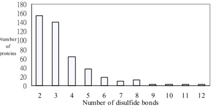
After this filtering procedure, 452 proteins were selected and Fig. 3.1 shows the bar graph of the distribution of the proteins grouped according to the number of the disulfide bonds.
3.3 Results
A 4-fold cross validation was performed to exam the proposed approach. The data set was randomly split into four folds. In each iteration, one of the four folds was treated as the testing set, and the others as the training set. There are five models tested on these data.
Fig. 2 shows that the prediction accuracy rises when the window size increases. However, the effects are marginal when the window size exceeds 17. The results indicate that the amino acid type around the cysteine actually affects the formation of disulfide bonds. However, when too many residues around the cysteine, including no particular information on the formation of a disulfide bond, were considered, predictions would be affected by these noises.
0 20 40 60 80 100 120 140 160 180 2 3 4 5 6 7 8 9 10 11 12
Number of disulfide bonds
Number of proteins
disulfide bonds. Most proteins have less than six disulfide bonds. 15 20 25 30 35 40 45 50 3 5 7 9 11 13 15 17 19 21 Window size (n ) P re di ct ion accuracy (%) Wn Wn+Pss
Figure 3.2 The overall accuracy Qp of model Wn and Wn+Pss with different window size n.
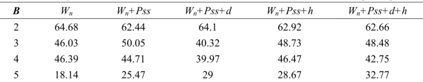
Two measurements, Qp and Qt, as described in Section 2.2, are used herein to evaluate those five
models. Table 3.1 and table 2 show the results. The overall best model is W17+Pss, which exhibits Qp
= 44.53% accuracy. This model is based on the features of amino acid type and predicted secondary structures. W17+Pss performs slightly better than W17 by considering predicted secondary structures.
According to Fig. 3.3, the ratios of predicted secondary structure pairs are different in three types. Cysteines at β-sheet prefer to form disulfide-bond with cysteines at coil or α-helix, rather than β-sheet. Cysteines at α-helix prefer to form disulfide-bond with cysteines at coil. These differences contribute slightly to the improvement of prediction (Fig. 3.2).
Table 3.3 shows the comparison between the results of the proposed method with Farselli et al.’s and Vullo et al.’s methods. Farselli equated the problem to a problem of finding the maximum weight perfect matching in a weighted complete graph according to a matrix of contact potential. They trained potential matrix by Edmonds-Gabow algorithm and Monte-Carlo simulated annealing. Vullo and Frasconi scored the candidate graphs which represent possible disulfide connectivity patterns by using recursive neural networks. Please note that their data sets were extracted from SwissProt release no. 39, while ours was from no. 40. But all the criteria for selecting protein sequences in SwissProt database are identical.
Table 3.1 The Qp of different models, the window size n of feature Wn is 17 according to Fig. 3.2. B Wn Wn+Pss Wn+Pss+d Wn+Pss+h Wn+Pss+d+h 2 64.68 62.43 64.1 62.92 62.66 3 34.63 39.17 29.01 37.15 35.87 4 36.54 32.74 30.72 31.32 28.03 5 2.27 7.83 7.08 8.15 3.45 avg 43.05 44.53 41.01 43.87 42.34
Table 3.2 The Qt of different models, the window size n of feature Wn is 17 according to Fig. 3.2. B Wn Wn+Pss Wn+Pss+d Wn+Pss+h Wn+Pss+d+h
2 64.68 62.44 64.1 62.92 62.66
3 46.03 50.05 40.32 48.73 48.48
4 46.39 44.71 39.97 46.47 42.75
avg 46.52 48.59 44.74 49.11 48.12 0 0.05 0.1 0.15 0.2 0.25 H E C H E C
Figure 3.3 The ratio of the predicted secondary structure pairs for disulfide-bonded cysteines. H, E, and C represent α-helix, β-sheet, and random coil, respectively. Cysteines have different favors for
forming disulfide bond in each secondary structure types.
Table 3.3 shows that the proposed method yields higher overall prediction accuracy than the other two methods. Our approach used various combinations of features while they only consider the amino acid type. Besides, larger window size is considered to retain more information from the sequences.
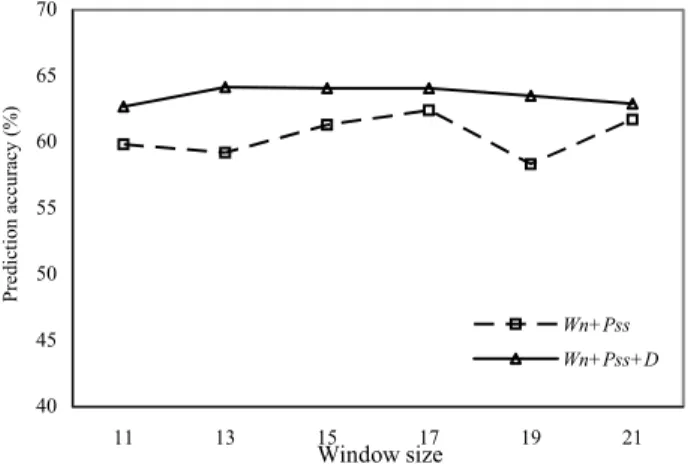
In model Wn+Pss+D, the addition of sequence distance makes it perform better than the other
models for proteins with two disulfide bonds (B = 2). Fig. 4 shows the comparison of Wn+Pss and Wn+Pss+D. According to the figure, disulfide connectivity patterns of proteins with two disulfide
bonds have strong preference for some specific patterns.
Adding the feature H, the prediction accuracy for proteins with five disulfide bonds is better than the other models (Fig. 5), probably due to those more non-local contacts, such as hydrophobic/hydrophilic interactions, occur in this group of proteins.
An interesting result is that although the model Wn+Pss+H+D combines all features, it does not
yield the best. From above analysis, the feature H and D can contribute to improving the prediction in different groups. However these two features possibly interfere with each other and combining these two features does not perform as well as expected. Another possibility is that different weight of these features should be considered.
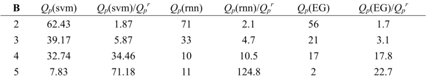
Table 3.3 Comparison between the proposed method and Farselli’s, Vullo’s method, where Qp(svm)
is the prediction accuracy for SVM-based method, Qp(rnn) is the accuracy for Vullo’s method (RNN), Qp(EG) is the accuracy for Farselli’s method (Edmond-Gabow), Qp(svm)/Qpr is the times to a
random predictor for a SVM-based method, and vice versa. The number in first column is the number of disulfide bonds B.
B Qp(svm) Qp(svm)/Qpr Qp(rnn) Qp(rnn)/Qpr Qp(EG) Qp(EG)/Qpr
2 62.43 1.87 71 2.1 56 1.7
3 39.17 5.87 33 4.7 21 3.1
4 32.74 34.46 10 10.5 17 17.8
Avg 44.53 2.87 39 30.35 2.18 40 45 50 55 60 65 70 11 13 15 17 19 21 Window size P redi ct io n accuracy (%) Wn+Pss Wn+Pss+D
Figure 3.4 The Qp of Wn+Pss and Wn+ Pss +D when B = 2 with different window sizes.
3.4 Conclusions
We have proposed a method to predict disulfide connectivity using support vector mechanism (SVM) and pattern matching algorithm. The corresponding accuracy (overall Qp = 44.53%) is
comparable or better than other published methods. In addition to consider amino-acid type features, predicted secondary structures, hydrophobicity, sequential distance feature are explored. The overall accuracy rises if the predicted secondary structures are considered. Two interesting results are also investigated in this paper. First, when the number of disulfide bonds is large (for example, five), the accuracy will significantly improved when we consider the feature of hydrophobicity. Second, when the number of disulfide bonds is small (for example, two), the feature sequential distance will help the predictor to obtain higher accuracy. In the future, we will pursue the proposed approach in adding more biological features, for example the evolutionary information. Different weight of these features should also be considered.
0 2 4 6 8 10 12 14 16 18 20 11 13 15 17 19 21 Window size Pr ed ict ion accu racy ( % ) Wn+Pss Wn+Pss+H
Figure3.5 The Qp of Wn+Pss and Wn+Pss+H when B = 5 with different window sizes.
4. Amber function chip Implementation
. In this project, we will build a distributed computation machine similar to IBM's BlueGene™, yet much more inexpensive, based on available technologies.Currently, microbiological scientists, who wish to research problems related to chemical properties of proteins, have to determine the structures and sequences of each protein molecules in the chain of reactions. These molecules can be very complex and large, requiring supercomputers days of calculation, if not
years and millenniums. Such long processing time is not acceptable. We have decided to combine current technologies, which are commonly available, into a fast, powerful solution to predict protein folding.
With some industrial experienced members in our team, we take the FPGA way rather than the fabrication way. FPGA is a reconfigurable solution to implement some high-speed digital designs which are not widely used. With nonstop growth of market, FPGA may be the second 0.13um semiconductor product in the world, just ranked below Intel Pentium processor. We may expect FPGA to be listed as number one as well as successive Intel processor.
Keeping our complicated goal as simple as possible, we have strived to maintain simplicity while slightly over-engineering the product to prevent failure. The user inputs analytical data into her GUI client to the data distribution server (DDS). The DDS divides the data up into calculating sizes, sends the data over 100mbit/1000mbit Ethernet to available data calculation unit (DCU). The DCU, being a thin-client computer with a few specially designed ASIC onboard, makes the calculations, and returns the data to the DDS.
Our main backbone of communication will be optical/copper gigabit Ethernet. Should there be any requirement of higher bandwidth, we will switch to commercially available solutions such as ATM (Asynchronous Transfer Mode) networks or fiber-channels.
We will implement our ASIC (Application Specific Integrated Circuit) on the modern Xilinx™ VertexII™ FPGA (Field Programmable Gate Array), packaged onto a PCB (Printed Circuit Board) with PCI (Peripheral Component Interconnect) connectors. It will include a pipelined algorithm of the Amber Force-field implementation, called Amber7™. The copyright of Amber7 belongs to the University of California Regents, and we will procure the usage rights from the U.C. Regents.
To implement a digital system that would deal with energy equations, we need iteration architecture to loop data in such data pathway. The central controller loops data between data registers, and operators. There is still another key to accelerate the computing speed, and the parallel architecture shows clues. The performance is speeded up N times with N operation units, with well arranged data pathways.
To reduce the difficulties of learning to use our system, we try to implement our system with the main stream PC products as often as possible. The final system will be a PC-based hardware, not a supercomputer nor an expensive work station.
For the sake of being reconfigurable, this FPGA hardware provides us not only a platform to implement Amber algorithm, but also a highway to some deep computing problems in bioinformatics.
The figure above shows the board level design of our system. The PCI provides a fast and popular interface for chips to receive data and command from PC.
This figure reveals the most basic data flow in our system, assuming the data of Ligand and Receptor comes from external data storage with well-scheduled data dispatcher. However, to make the diagram simple, the architecture of main operators is not drawn.
We have now completed the hardware design phase of the NTUGene project. We are proud to have designed a 400MHz PCB (Printed Circuit Board) with almost no electromagnetic interference. The PCB, now working with several features and demonstrated internally, including: (per board)
1. Two 500MHz state-of-the-art FPGAs not available on the market yet 2. Two 13Gigabits/sec LVDS-based interconnect
3. Four 2.5Gigabits/sec RocketIO-based interconnect 4. One PCI 1.1 interface
5. One 400MHz DDR SDRAM slot, capable of taking up to 1GB of memory 6. Two banks of 32MB of 200MHz SRAM, not available on the market yet
These achievements are comparable to the best designs on the market, and we have achieved them with minimal staffing, compared to large-scale PCB design houses.
We are now in the final design phase of the project, completing the data routing software, the user interface, and the firmware. We now plan to show a complete demo before the end of July, which would be the end of the 2nd year in this NSC research project.
七、 參考文獻:
1. Aaron R. Dinner and Martin Karplus. (1999) Is Protein Unfolding the Reverse of Protein Folding? A Lattice Simulation Analysis. J. Mol Biol. ,292, 403-419
2. Abagyan,R.A. (1993) Towards protein folding by global energy optimization. FEBS Letters, 325, 17-h.
Energetics, Function and Folding: Simulations and Bioinformatics Analysis. J. Mol. Biol. , 300, 975-985
4. Andrej Sali, Eugene Shakhnovich and Martin Karplus,(1994) Kinetics of Protein Folding: A Lattice Model Study of the Requirements for Folding to the Native State. J. Mol. Biol., 235, 1614-1636
5. Anfinsen,C.B.(1973) Principles that govern the folding of protein chains. Science., 181, 223-230.
6. Anfinsen,C.B., Haber,E., Sela,M. & White,F.H. (1961) The kinetics of formation of native ribonuclease during oxidation of the reduced polypeptide chain. Proc. Nat. Acad. Sci., U.S.A. 47, 1309-1314.
7. Broglia,R.A. and Tiana,G. (2001) Reading the Three-Dimensional Structure of Lattice Model-Designed Proteins from Their Amino Acid Sequence. PROTEINS: Structure, Function, and Genetics, 45, 421-427
8. Brower,R.C., Vasmatzis,C., Silverman,M. & Delisi,C. (1993) Exhaustive conformational search and simulated annealing models of lattice peptides. Biopolymers. 33, 329-334.
9. Carl Branden and John Tooze, Introduction to Protein Structure.(Second Edition), GARLAND.
10. Covell,D.G. (1994) Lattice Model Simulations of Polypeptide Chain Folding. J.Mol.Biol.,235,1032-1043
11. Covell,D.G. and Jernigan,R.L. (1990) Conformations of folded proteins in restricted spaces. Biochemistry, 29, 3287-3294
12. Crippen. G. M. (1991) Prediction of protein folding from amino acid sequence over discrete conformation spaces. Biochemistry, 30, 4232-4237.
13. David A. Hinds and Michael Levitt (1994) Exploring Conformational Space with a Simple Lattice Model for Protein Structure. J. Mol. Biol. 243, 668-682
14. Go,N. and Taketomi,H. (1978) Respective roles of short-and long-range interactions in protein folding. Proc. Nat. Acad. Sci., U.S.A., 75, 559-563.
15. Hongyu Zhang (2002) Protein Tertiary Structures: Prediction from Amino Acid Sequence. ENCY CLOPEDIA of LIFE SCIENCES.
16. Jinn-Moon Yang (2001) A Family Competition Evolutionary Approach of Global Optimization in Neural Networks, Optical Thin-film Design, and Structure-based Drug Design.
17. Junni L. Zhang and Jun S. Liu (2002) A new sequential importance sampling method and its application to the two-dimensional hydrophobic-hydrophilic model. Journal of Chemical Physics, Volume 117, Number 7 , 3492-3498
18. Kaizhi Yue, Klaus M. Fiebig, Paul D. Thomas, Hue Sun Chan. (1995) A test of lattice protein folding algorithms. Proc. Natl. Acad. U.S.A., Vol.92, 325-329.
19. Kuntz,I., Crippen,G., Kollman,P., Kimelman,D. (1976) Calculation of protein tertiary structure. J. Mol. Biol. ,106:983-994.
20. Lau,K.F. & Dill,K.A. (1989) Lau KF, Dill KA. Lattice statistical mechanics model of the conformational and sequence spaces of proteins. Macromolecules ,22:3986-3997.
21. Levinthal,C. (1968) Are there pathways for protein folding ? J. Chem. Phys., 65, 44-45.
22. Levitt,M. (1976) Simplified representations of protein conformations for rapid simulation of protein folding. J. Mol. Biol. ,104, 59-107.
23. Levitt,M. & Warshel,A. (1975) Computer simulation of protein folding. Nature, 253, 694-698.
24. MaiSua Li, D. K. Klimov, D. Thirumalai (2002) Folding in lattice models with side chains., Computer Physics Communications., 147 , 625-628
25. Oswin Aichholzer, David Bremner, Eric D. Demaine, Henk Meijer, Vera Sacristan, Michael Soss (2003) Long proteins with unique optimal foldings in the H-P model. Computational Geometry, 25 , 139-159
26. Ramakrishnan,R., Ramachandran,B., Pekney,J.F. (1997) A dynamic Monte Carlo algorithm for exploration of dense conformational spaces in heteropolymers. J. Chem. Phys.,106:2418-2425 27. Rolf Backofen, Sebastain Will and Erich Bornberg-Bauer, (1999) Application of constraint
programming techniques for structure prediction of lattice proteins with extended alphabets., BIOINFORMATICS, Vol. 15 no.3, 234-242
28. Ron Unger and John Moult (1993) Genetic Algorithms for Protein Folding Simulations. J.Mol. Biol, 231, 75-81
29. Skolnick,J. & Kolinski.A. (1990) Simulations of the folding of a globular protein. Science, 250, 1121-1125.
30. Skolnick,J., Kolinski,A., Brooks,C.L. III. Godzik,A. & Rey,A. (1993) A method for predicting protein structure from sequence. Curr. Biol. ,3, 414-423.
31. Tianzi Jiang and Qinghua Cui, (2003) Protein folding simulations of the hydrophic-hydrophlic model by combining tabu search with genetic algorithm. Journal of Chemical physics. Volume 119,Number 8
32. Ugo Bastolla, Helge Frauenkron, Erwin Gerstner, Peter Grassberger and Walter Nadler (1998) Testing a New Monte Carlo Algorithm for Protein Folding. PROTEINS: structure, Function and Genetics , 32 , 52-66
33. Unger,R. and Moult,J. (1993) A Genetic Algorithm for 3D Protein Folding Simulations. Proceedings of the Fifth International Conference on Genetic Algorithms (ICGA'93), 581-588 34. Unger,R. and Moult,J. (1993) Genetic Algorithms for Protein Folding Simulations. J. Mol. Biol.
231, 75-81
35. Wetlaufer,D.B. (1973) Nucleation, rapid folding, and globular intrachain regions in proteins. Proc. Natl. Acad. Sci. U.S.A., 70,697-701
36. Wilson,C., Doniach,S. (1989) A computer model to dynamically simulate protein folding: Studies with crambin. Proteins Struct Funct Genet 6:193-209.
37. Zhdannov,V.P. and Kasemo,B. (1997) Monte Carlo Simulation of Protein Folding Whit Orientation-Dependent Monomer-Monomer Interaction. Protein : Structure, Function, and Genetics 29:508-516