Abstract—This study presents a functional-link-based fuzzy neural network (FLFNN) structure for temperature control. The proposed FLFNN controller uses functional link neural networks (FLNN) that can generate a nonlinear combination of the input variables as the consequent part of the fuzzy rules. An online learning algorithm, which consists of structure learning and parameter learning, is also presented. The structure learning depends on the entropy measure to determine the number of fuzzy rules. The parameter learning, based on the gradient descent method, can adjust the shape of the membership function and the corresponding weights of the FLNN. Simulation result of temperature control has been given to illustrate the performance and effectiveness of the proposed model.
I. INTRODUCTION
HE concept of fuzzy neural network (FNN) for control problem has been grown into a popular research topic in recent years [1]-[4]. The reason is that classical control theory usually requires a mathematical model for designing the controller. The inaccuracy of mathematical modeling of plants usually degrades the performance of the controller, especially for nonlinear and complex control problems [5]. On the contrary, the FNN controller offers a key advantage over traditional adaptive control systems. The FNN do not require mathematical models of plants. The FNN bring the low-level learning and computational power of neural networks into fuzzy systems and give the high-level human-like thinking and reasoning of fuzzy systems to neural networks.
This study presents a functional-link-based fuzzy neural network (FLFNN) structure for temperature control. The FLFNN controller, which combines a fuzzy neural network (FNN) with functional link neural network (FLNN) [6]-[7], is designed improve the accuracy of functional approximation. Each fuzzy rule that corresponds to a FLNN consists of functional expansion of the input variables. The orthogonal polynomials and linearly independent functions are adopted as functional link neural network bases. An online learning algorithm, consisting of structure learning and parameter learning, is proposed to construct the FLFNN model automatically. The structure learning algorithm determines whether or not to add a new node which satisfies the fuzzy C. H. Chen and C. T. Lin are with the Dept. of Electrical and Control Engineering, National Chiao-Tung University, Hsinchu 300, Taiwan, R.O.C. C. J. Lin is with the Dept. of Computer Science and Information Engineering, Chaoyang University of Technology, No.168, Jifong E. Rd., Wufong Township, Taichung County 41349, Taiwan, R.O.C.
*Corresponding author. (E-mail: chchen.ece93g@nctu.edu.tw)
partition of the input variables. Initially, the FLFNN model has no rules. The rules are created automatically by entropy measure. The parameter learning algorithm is based on backpropagation to tune the free parameters in the FLFNN model simultaneously to minimize an output error function.
The characteristics of the proposed FLFNN model are explained as follows. First, the consequent of the fuzzy rules is a nonlinear combination of the input variables. This study uses the functional link neural network to the consequent part of the fuzzy rules. The functional expansion in FLFNN model can yield the consequent part of a nonlinear combination of input variables. Second, the online learning algorithm can automatically construct the FLFNN model. No rules or memberships exist initially. They are created automatically as learning proceeds, as online incoming training data are received and as structure and parameter learning are performed. Third, as demonstrated in section IV, the FLFNN model is a more adaptive and effective controller than the other methods.
II. STRUCTURE OF FLFNN
This section describes the structure of functional link neural networks and the structure of the FLFNN model. In functional link neural networks, the input data usually incorporate high order effects and thus artificially increase the dimensions of the input space. Accordingly, the input representation is enhanced and linear separability is achieved in the extended space. The FLFNN model adopted the functional link neural network generating complex nonlinear combination of the input variables as the consequent part of the fuzzy rules. The rest of this section details these structures.
A. Functional Link Neural Networks
The functional link neural network is a single layer network in which the need for hidden layers is eliminated. While the input variables generated by the linear links of neural networks are linearly weighted, the functional link acts on an element of input variables by generating a set of linearly independent functions, which are suitable orthogonal polynomials for a functional expansion, and then evaluating these functions with the variables as the arguments. Therefore, the FLNN structure considers trigonometric functions. For example, for a two-dimensional input [x x ]T
2 1 =
X ,
enhanced data are obtained using trigonometric functions as
T ,... x cos , x sin , x ,..., x cos , x sin , x , ( ) ( ) ( ) ( ) ] 1 [ 1 π 1 π 1 2 π 2 π 2 = Φ .
A Functional-Link-Based Fuzzy Neural Network
for Temperature Control
Cheng-Hung Chen*, Chin-Teng Lin, Fellow, IEEE, and Cheng-Jian Lin, Member, IEEE
Thus, the input variables can be separated in the enhanced space [8]. In the FLNN structure with reference to Fig. 1, a set of basis functions Φ and a fixed number of weight parameters W represent fW(x). The theory behind the FLNN for multidimensional function approximation has been discussed elsewhere [6] and is analyzed below.
x1 x2 F.E. . . . xN . . . . . . . . . 1 φ 2 φ M φ ∑ ∑ ∑ ' ˆ1 y ' ˆ2 y ' ˆm y 1 ˆy 2 ˆy m yˆ X W Y ˆ Fig. 1. Structure of FLNN.
Consider a set of basis functions Β={φk∈Φ(A)}k∈Κ , }
2 1 {, ,...
=
Κ with the following properties; 1) φ1=1, 2) the
subset M
k j ={ ∈Β}k=1
Β φ is a linearly independent set, meaning that if
∑
M= =k1wkφk 0 , then wk =0 for all
M ..., , , k=12 , and 3)
[
∑
]
<∞ = 2 1 1 2 / j k k A j sup φ . Let M k M ={ }k 1=Β φ be a set of basis functions to be considered, as shown in Fig. 1. The FLNN comprises M basis
functions {φ1,φ2,...,φM}∈ΒM. The linear sum of the jth node
is given by
∑
= = M k k kj j w ( ) yˆ 1 X φ (1) where X∈Α⊂ℜN, T N x x x, ,..., ] [ 1 2 =X is the input vector
and T jM j j T j =[w1,w2,...,w ]
W is the weight vector associated
with the jth output of the FLNN. yˆj denotes the local output
of the FLNN structure and the consequent part of the jth fuzzy
rule in the FLFNN model. Thus, Eq.(1) can be expressed in
matrix form as yˆj =WjΦ , where
T M x ... x x), ( ), , ( )] ( [φ1 φ2 φ
Φ = is the basis function vector,
which is the output of the functional expansion block. The
m-dimensional linear output may be given by yˆ= WΦ,
where T m yˆ ... yˆ yˆ ˆ =[ 1, 2, , ]
y , m denotes the number of
functional link bases, which equals the number of fuzzy rules in the FLFNN model, and W is a (m×M)-dimensional weight
matrix of the FLNN given by T
m w w w, ,..., ] [ 1 2 = W . The jth
output of the FLNN is given by yˆj'=ρ(yˆj), where the
nonlinear function ρ
( )
⋅ =tanh( )
⋅ . Thus, the m-dimensional output vector is given by) ( ) ˆ ( ˆ f x W y Y=ρ = (2) where Yˆ denotes the output of the FLNN. In the FLFNN model, the functional link bases do not exist in the initial state, and the amount of functional link bases generated by the online learning algorithm is consistent with the number of fuzzy rules. Section III details the online learning algorithm.
B. Structure of FLFNN Controller
This subsection describes the FLFNN model, which uses a nonlinear combination of input variables (FLNN). Each fuzzy rule corresponds to a sub-FLNN, comprising a functional link. Figure 2 presents the structure of the proposed FLFNN model. Nodes in layer 1 are input nodes, which represent input variables. Nodes in layer 2 are called membership function nodes and act as membership functions, which express the input fuzzy linguistic variables. Nodes in this layer are adopted to determine Gaussian membership values. Each node in layer 3 is called a rule node. Nodes in layer 3 are equal to the number of fuzzy sets that correspond to each external linguistic input variable. Links before layer 3 represent the preconditions of the rules, and links after layer 3 represent the consequences of the rule nodes. Nodes in layer 4 are called consequent nodes, each of which is a nonlinear combination of the input variables. The node in layer 5 is called the output node; it is recommended by layers 3 and 4, and acts as a defuzzifier.
The FLFNN realizes a fuzzy if-then rule in the following form.
Rule-j: IFx1isA1jandx2isA2j...andxiisAij...andxNisANj
M Mj j j M k k kj j w ... w w w yˆ φ φ φ φ + + + = =
∑
= 2 2 1 1 1 THEN (3) where xi and yˆj are the input and local output variables, respectively; Aij is the linguistic term of the precondition part with Gaussian membership function; N is the number of input variables; wkj is the link weight of the local output; φk is the basis trigonometric function of the input variables; M is the number of basis function, and Rule-j is the jth fuzzy rule.The operation functions of the nodes in each layer of the FLFNN model are now described. In the following description, u(l) denotes the output of a node in the lth layer.
x1 x2 F.E. x1 x2 y w11 w21 wM1 . . . . . . . . . . . . . . .
Layer 1 Layer 2 Layer 3 Layer 4 Layer 5
Norma liz ati on 1 ˆy 2 ˆy 3 ˆy 1 φ 2 φ M φ ∑ ∑ ∑
Fig. 2. Structure of proposed FLFNN model.
Layer 1 (Input node): No computation is performed in this
corresponds to one input variable, and only transmits input values to the next layer directly:
i ) (
i x
u1 = . (4)
Layer 2 (Membership function node): Nodes in this layer
correspond to a single linguistic label of the input variables in layer 1. Therefore, the calculated membership value specifies the degree to which an input value belongs to a fuzzy set in layer 2. The implemented Gaussian membership function in layer 2 is ⎟ ⎟ ⎠ ⎞ ⎜ ⎜ ⎝ ⎛ − − = 2 2 1 2 [ ] ij ij ) ( i ) ( ij m u exp u σ (5) where mij and σij are the mean and variance of the Gaussian membership function, respectively, of the jth term of the ith input variable xi.
Layer 3 (Rule Node): Nodes in this layer represent the
preconditioned part of a fuzzy logic rule. They receive one-dimensional membership degrees of the associated rule from the nodes of a set in layer 2. Here, the product operator described above is adopted to perform the IF-condition matching of the fuzzy rules. As a result, the output function of each inference node is
∏
= i ) ( ij ) ( j u u3 2 (6) where the∏
i ) ( iju 2 of a rule node represents the firing strength of its corresponding rule.
Layer 4 (Consequent Node): Nodes in this layer are called
consequent nodes. The input to a node in layer 4 is the output from layer 3, and the other inputs are nonlinear combinations of input variables from a functional link neural network, where the nonlinear combination function has not used the function tanh
( )
⋅ , as shown in Fig. 2. For such a node,∑
= ⋅ = M k k kj ) ( j ) ( j u w u 1 3 4 φ (7)where wkj is the corresponding link weight of functional link neural network and φk is the functional expansion of input variables. The functional expansion uses a trigonometric polynomial basis function, given by
[
x1sin(πx1) cos(πx1 )x2sin(πx2 )cos(πx2)]
fortwo-dimensional input variables. Therefore, M is the number of basis functions, M= 3×N, where N is the number of input variables.
Layer 5 (Output Node): Each node in this layer
corresponds to a single output variable. The node integrates all of the actions recommended by layers 3 and 4 and acts as a defuzzifier with,
∑
∑
∑
∑
∑
∑
∑
= = = = = = = = ⎟ ⎠ ⎞ ⎜ ⎝ ⎛ = = = R j ) ( j R j j ) ( j R j ) ( j R j M k k kj ) ( j R j ) ( j R j ) ( j ) ( u yˆ u u w u u u u y 1 3 1 3 1 3 1 1 3 1 3 1 4 5 φ (8)where R is the number of fuzzy rules, and y is the output of the FLFNN model.
III. Learning Algorithms of the FLFNN Controller This section presents an online learning algorithm for constructing the FLFNN model. The proposed learning algorithm comprises a structure learning phase and a parameter learning phase.
A. Structure Learning Phase
The first step in structure learning is to determine whether a new rule from should be extracted the training data and to determine the number of fuzzy sets in the universal of discourse of each input variable, since one cluster in the input space corresponds to one potential fuzzy logic rule, in which
ij
m and σij represent the mean and variance of that cluster, respectively. For each incoming pattern x, the rule firing strength can be regarded as the degree to which the incoming pattern belongs to the corresponding cluster. For computational efficiency, the measure criterion calculated from ( )
ij
u2 is adopted as the entropy measure
∑
= − = N i ij ij j D log D EM 1 2 (9) where =( )
(2 −)1 ij ij expuD and EMj∈[0,1]. According to Eq.(9),
the criterion for generating a new fuzzy rule and new functional link bases for new incoming data is described as follows. The maximum entropy measure
j R j max maxEM EM ) T ( ≤ ≤ = 1 (10)
is determined, where R(t) is the number of existing rules at time t. If EMmax≤EM then a new rule is generated, where
] 1 0 [ ,
EM∈ is a prespecified threshold that decays during the learning process.
In the structure learning phase, the threshold parameter
EM is an important parameter. The threshold is set to between zero and one. A low threshold leads to the learning of coarse clusters (i.e., fewer rules are generated), whereas a high threshold leads to the learning of fine clusters (i.e., more rules are generated). If the threshold value equals zero, then all the training data belong to the same cluster in the input space. Therefore, the selection of the threshold value EM
will critically affect the simulation results, and this value will be based on practical experimentation or on trial-and-error tests. EM is defined as 0.26-0.3 times the input variance.
Once a new rule has been generated, the next step is to assign the initial mean and variance for the new membership function and the corresponding link weight for the consequent part. Since the goal is to minimize an objective function, the mean, variance and weight are all adjustable later in the parameter learning phase. Hence, the mean, variance and weight for the new rule are set as follows;
i ) R ( ij x m (t+ 1) = (11) init ) R ( ij ) t ( σ σ +1 = (12) ] 1 1 [ 1 random , w(R ) kj ) t (+ = − (13)
where xi is the new input and σinit is a prespecified constant. The whole algorithm for the generation of new fuzzy rules and fuzzy sets in each input variable is as follows. No rule is assumed to exist initially exist:
Step 1: IF xi is the first incoming pattern THEN do {Generate a new rule
with mean mi1=xi, variance σi1=σinit, weight wk1=random[−1,1]
where σinit is a prespecified constant. }
Step 2: ELSE for each newly incoming xi, do {Find EMmax maxjR EMj
) t ( ≤ ≤ = 1 IF EMmax≥EM do nothing ELSE {R(t+1) = R(t) +1
generate a new rule with mean i R ij x m(t+1) = , variance init R ij ) t ( σ σ + 1 = , weight wR(t1) random[ 1,1] kj = − +
where σinit is a prespecified constant.} }
B. Parameter Learning Phase
After the network structure has been adjusted according to the current training data, the network enters the parameter learning phase to adjust the parameters of the network, optimized according to the same training data. The learning process involves determining the minimum of a given cost function. The gradient of the cost function is computed and the parameters are adjusted along the negative gradient. The backpagation algorithm is adopted for this supervised learning method. When the single output case is considered for clarity, the goal to minimize the cost function E is defined as ) ( 2 1 )] ( ) ( [ 2 1 ) (t yt y t 2 e2t E = − d = (14) where yd(t) is the desired output and y(t) is the model output for each discrete time t. In each training cycle, starting at the input variables, a forward pass is adopted to calculate the activity of the model output y(t).
When the backpropagation learning algorithm is adopted, the weighting vector of the FLFNN model is adjusted such that the error defined in Eq.(14) is less than the desired threshold value after a given number of training cycles. The well-known backpropagation learning algorithm may be written briefly as ⎟⎟ ⎠ ⎞ ⎜⎜ ⎝ ⎛ ∂ ∂ − + = Δ + = + ) ( ) ( ) ( ) ( ) ( ) 1 ( t W t E t W t W t W t W η (15)
where, in this case, η and W represent the learning rate and the tuning parameters of the FLFNN model, respectively. Let
T
w , , m
W=[ σ ] be the weighting vector of the FLFNN model.
Then, the gradient of error E(⋅) in Eq.(14) with respect to an arbitrary weighting vector W is
W t y t e W ) t E ∂ ∂ = ∂ ∂ () ) ( ( . (16) Recursive applications of the chain rule yield the error term for each layer. Then the parameters in the corresponding layers are adjusted. With the FLFNN model and the cost function as defined in Eq.(14), the update rule for wj can be derived as follows; ) ( ) ( ) 1 (t w t w t wkj + = kj +Δ kj (17) where ⎟⎟ ⎟ ⎠ ⎞ ⎜⎜ ⎜ ⎝ ⎛ ⋅ ⋅ − = ∂ ∂ − = Δ
∑
= R j ) ( j k ) ( j w kj w kj u u e w E t w 1 3 3 ) ( φ η η .Similarly, the update laws for mij, and σij are ) ( ) ( ) 1 (t m t m t mij + = ij +Δ ij (18) ) ( ) ( ) 1 (t ij t ij t ij σ σ σ + = +Δ (19) where ⎟ ⎟ ⎠ ⎞ ⎜ ⎜ ⎝ ⎛ − ⋅ ⎟⎟ ⎟ ⎠ ⎞ ⎜⎜ ⎜ ⎝ ⎛ ⋅ ⋅ − = ∂ ∂ − = Δ
∑
= 2 1 1 3 4 2( ) ) ( ij ij ) ( i R j ) ( j ) ( j m ij m ij m u u u e m E t m σ η η ⎟ ⎟ ⎠ ⎞ ⎜ ⎜ ⎝ ⎛ − ⋅ ⎟⎟ ⎟ ⎠ ⎞ ⎜⎜ ⎜ ⎝ ⎛ ⋅ ⋅ − = ∂ ∂ − = Δ∑
= 3 2 1 1 3 4 2( ) ) ( ij ij ) ( i R j ) ( j ) ( j ij ij m u u u e E t σ η σ η σ σ σwhere ηw, ηm and ησ are the learning rate parameters of the
weight, the mean, and the variance, respectively. IV. Control of Water Bath Temperature System The goal of this section is to elucidate the control of the temperature of a water bath system according to,
C T t y Y C t u dt ) t dy R ) ( ) ( ( = + 0− (20)
where y(t) is the output temperature of the system in °C ; u(t) is the heat flowing into the system; Y0 is room temperature; C
is the equivalent thermal capacity of the system, and TR is the equivalent thermal resistance between the borders of the system and the surroundings.
TR and C are assumed to be essentially constant, and the system in Eq.(20) is rewritten in discrete-time form to some reasonable approximation. The system
0 40 5 0 ( ) [1 ] 1 ) 1 ( ) ( ) 1 (k u k e y e e k y e y Ts ) k ( y . Ts Ts α α α α δ − − − − + − + − + = + (21)
is obtained, where α and δ are some constant values of TR and C. The system parameters used in this example are
4 0015 1 − = . e α , δ =8.67973e−3 and 0 Y=25.0 ( C° ), which were obtained from a real water bath plant considered elsewhere [9]. The input u(k) is limited to 0, and 5V represent voltage unit. The sampling period is Ts=30.
The conventional online training scheme is adopted for online training. Figure 4 presents a block diagram for the conventional online training scheme. This scheme has two phases - the training phase and the control phase. In the training phase, the switches S1 and S2 are connected to nodes 1 and 2, respectively, to form a training loop. In this loop, training data with input vector I(k)=[yp(k+1) yp(k)] and
desired output can be defined, where the input vector of the FLFNN controller is the same as that used in the general inverse modeling [10] training scheme. In the control phase, the switches S1 and S2 are connected to nodes 3 and 4, respectively, forming a control loop. In this loop, the control signal uˆ(k) is generated according to the input vector
)] ( ) 1 ( [ ) (k y k y k '
I = ref + p , where yp is the plant output and yref is the reference model output.
A sequence of random input signals urd(k) limited to 0 and
5V is injected directly into the simulated system described in
Eq.(21), using the online training scheme for the FLFNN controller. The 120 training patterns are selected based on the input-outputs characteristics to cover the entire reference output. The temperature of the water is initially 25 c° , and rises progressively when random input signals are injected. After 10000 training iterations, four fuzzy rules are generated. The obtained fuzzy rules are as follows.
Rule-1: IFx1isμ(32.416,11.615)andx2isμ(27.234,7.249) ) ( 35.204 ) ( 799 41 026 17 ) ( 546 34 ) ( 849 74 32.095 THEN 2 2 2 1 1 1 1 x cos x sin . x . x cos . x sin . x yˆ π π π π + − − − + = Rule-2: IFx1isμ(34.96,9.627)andx2isμ(46.281,13.977) ) ( 70.946 ) ( 61.827 52.923 ) ( 77.705 ) ( 11.766 21.447 THEN 2 2 2 1 1 1 2 x cos x sin x x cos x sin x yˆ π π π π + − − − + = Rule-3: IFx1isμ(62.771,6.910)andx2isμ(62.499,15.864) ) ( 103.33 ) ( 36.752 40.322 ) ( 46.359 ) ( 10.907 25.735 THEN 2 2 2 1 1 1 3 x cos x sin x x cos x sin x yˆ π π π π + + − − − = Rule-4: IFx1isμ(79.065,8.769)andx2isμ(64.654,9.097) ) ( 34.838 ) ( 61.065 5.8152 ) ( 57.759 ) ( 37.223 46.055 THEN 2 2 2 1 1 1 4 x cos x sin x x cos x sin x yˆ π π π π + + − − − = yp(k+1) yref(k+1) yp(k+1) 1 3 S1 Z-1 2 4 S2 ) ( ˆ k u ) (k u + Plant Z-1 – FLFNN Controller
Fig. 3. Conventional online training scheme.
This study compares the FLFNN controller to the PID controller [11], the manually designed fuzzy controller (FC) [3], the functional link neural network (FLNN) and the TSK-type fuzzy neural network (TSK-type FNN). Each of these controllers is applied to the water bath temperature control system. The performance measures include the
set-points regulation, the influence of impulse noise and a large parameter variation in the system.
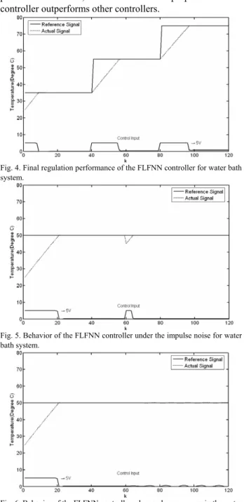
The first task is to control the simulated system to follow three set-points. ⎪ ⎩ ⎪ ⎨ ⎧ ≤ < ≤ < ≤ ° ° ° = . k k k for for for , c , c , c k yref 120 80 80 40 40 75 55 35 ) ( . (22)
Figure 4 presents the regulation performance of the FLFNN controller. We also test the regulation performance by using the FLNN controller and the TSK-type FNN controller. To test their regulation performance, a performance index, the sum of absolute error (SAE), is defined by
∑
− = k ref k yk y SAE ( ) ( ) (23) where yref(k) and y(k) are the reference output and theactual output of the simulated system, respectively. The SAE values of the FLFNN controller, the PID controller, the fuzzy controller, the FLNN controller and the TKS-type NFN controller are 352.8, 418.5, 401.5, 379.2 and 361.9, which are given in the second row of Table 1. The proposed FLFNN controller yields a much better SAE value of regulation performance than the other controllers.
The second set of simulations is performed to elucidate the noise-rejection ability of the five controllers when some unknown impulse noise is imposed on the process. One impulse noise value −5°C is added to the plant output at the sixtieth sampling instant. A set-point of 50°C is adopted in this set of simulations. For the FLFNN controller, the same training scheme, training data and learning parameters as were used in the first set of simulations. Figure 5 presents the behaviors of the FLFNN controller under the influence of impulse noise. The SAE values of the FLFNN controller, the PID controller, the fuzzy controller, the FLNN controller and the TSK-type FNN controller are 270.4, 311.5, 275.8, 324.51 and 274.75, which are shown in the third row of Table 1. The FLFNN controller performs quite well. It recovers very quickly and steadily after the presentation of the impulse noise.
One common characteristic of many industrial-control processes is that their parameters tend to change in an unpredictable way. The value of 0.7∗ ku( −2) is added to the plant input after the sixtieth sample in the third set of simulations to test the robustness of the five controllers. A set-point of 50°C is adopted in this set of simulations. Figure 6 presents the behaviors of the FLFNN controller when in the plant dynamics change. The SAE values of the FLFNN controller, the PID controller, the fuzzy controller, the FLNN controller and the TSK-type FNN controller are 263.3, 322.2, 273.5, 311.5 and 265.4, which values are shown in the fourth row of Table 1. The results present the favorable control and disturbance rejection capabilities of the trained FLFNN controller in the water bath system.
The results present the favorable control and disturbance rejection capabilities of the trained FLFNN controller in the
water bath system. The aforementioned simulation results, presented in Table 1, demonstrate that the proposed FLFNN controller outperforms other controllers.
Fig. 4. Final regulation performance of the FLFNN controller for water bath system.
Fig. 5. Behavior of the FLFNN controller under the impulse noise for water bath system.
Fig. 6. Behavior of the FLFNN controller when a change occurs in the water bath system.
V. Conclusion
This study proposes a functional-link-based neuro-fuzzy network (FLFNN) structure for temperature control. The FLFNN model uses the functional link neural network (FLNN) as the consequent part of the fuzzy rules. Therefore, the FLFNN model can generate the consequent part of a nonlinear combination of the input variables to be approximated more effectively. The FLFNN model can automatically construct and adjust free parameters by
performing online structure/parameter learning schemes concurrently. Finally, computer simulation results have shown that the proposed FLFNN controller has better performance than that of other models.
Table 1: Comparison of performance of various controllers.
FLFNN PID [11] FC [3] FLNN TSK-type FNN Regulation Performance 352.84 418.5 401.5 379.22 361.96 Influence of Impulse Noise 270.41 311.5 275.8 324.51 274.75 Effect of Change in Plant Dynamics 263.35 322.2 273.5 311.54 265.48 ACKNOWLEDGMENT
This research was sponsored by Department of Industrial Technology, Ministry of Economic Affairs, R.O.C. under the grant 95-EC-17-A-02-S1-029.
REFERENCES
[1] T. Takagi and M. Sugeno, “Fuzzy identification of systems and its applications to modeling and control,” IEEE Trans. on Syst., Man, Cybern., vol. 15, pp. 116-132, 1985.
[2] J.-S. R. Jang, “ANFIS: Adaptive-network-based fuzzy inference system,” IEEE Trans. on Syst., Man, and Cybern., vol. 23, pp. 665-685, 1993.
[3] C. T. Lin and C. S. G. Lee, Neural Fuzzy Systems: A Neuro-Fuzzy Synergism to Intelligent System, NJ: Prentice-Hall, 1996.
[4] C. F. Juang and C. T. Lin, “An on-line self-constructing neural fuzzy inference network and its applications,” IEEE Trans. Fuzzy Systems, vol. 6, no.1, pp. 12-31, Feb. 1998.
[5] K. J. Astrom and B. Wittenmark, Adaptive Control, MA: Addison-Wesley, 1989.
[6] J. C. Patra and R. N. Pal, “A functional link artificial neural network for adaptive channel equalization,” Signal Process, vol. 43, pp. 181-195, May 1995.
[7] J. C. Patra, R. N. Pal, B. N. Chatterji, and G. Panda, “Identification of nonlinear dynamic systems using functional link artificial neural networks,” IEEE Trans. on Syst., Man, and Cybern., vol. 29, Apr. 1999. [8] Y. H. Pao, Adaptive Pattern Recognition and Neural Networks, MA:
Addison-Wesley, 1989.
[9] J. Tanomaru and S. Omatu, “Process control by on-line trained neural controllers,” IEEE Trans. on Ind. Electron, vol. 39, pp. 511-521, 1992. [10] D. Psaltis, A. Sideris, and A. Yamamura, “A multilayered neural
network controller,” IEEE Contr. Syst., vol. 8, pp. 17–21, 1988. [11] C. L. Phillips and H. T. Nagle, Digital Control System Analysis and