Dynamic optimal groundwater management with inclusion of fixed costs

Dynamic Optimal Groundwater Management with Inclusion

of Fixed Costs

Chin-Tsai Hsiao

and Liang-Cheng Chang

Abstract: Obtaining optimal solutions for groundwater resources planning problems, while simultaneously considering both fixed costs and time-varying pumping rates, is a challenging task. Application of conventional optimization algorithms such as linear and nonlinear programming is difficult due to the discontinuity of the fixed cost function in the objective function and the combinatorial nature of assigning discrete well locations. Use of conventional discrete algorithms such as integer programming or discrete dynamic programming is hampered by the large computational burden caused by varying pumping rates over time. A novel procedure that integrates a genetic algorithm 共GA兲 with constrained differential dynamic programming 共CDDP兲 calculates optimal solutions for a groundwater resources planning problem while simultaneously considering fixed costs and time-varying pumping rates. The GA determines the number and locations of pumping wells with operating costs then evaluated using CDDP. This study demonstrates that fixed costs associated with installing wells significantly impact the optimal number and locations of wells.

DOI: 10.1061/共ASCE兲0733-9496共2002兲128:1共57兲

CE Database keywords: Genetic algorithm; Constrained differential dynamic programming; Groundwater management; Fixed cost.

Introduction

Groundwater, as an underground reservoir, is a valuable water resource with many diverse domestic, agricultural, and industrial uses. Owing to its importance, ensuring the sustainable use of groundwater has been extensively studied 共Gorelick 1983; Lin and Yang 1991; Yeh 1992; Pezeshk et al. 1994; Takahashi and Peralta 1995兲. Many optimization techniques have been employed in the planning stages of groundwater management, including lin-ear programming 共Aquado and Remson 1974; Molz and Bell 1977兲, nonlinear programming 共Murtagh and Saunders 1982; Gorelick et al. 1984; Ahlfeld et al. 1988a; b兲, mixed-integer pro-gramming 共Rosenwald and Green 1974兲, genetic algorithms 共McKinney and Lin 1994; Wang and Zheng 1998兲, and differen-tial dynamic programming 共DDP兲 共Jones et al. 1987兲. Among these methods, DDP significantly reduces the dimensionality dif-ficulties associated with nonlinear dynamic groundwater manage-ment problems共Jones et al. 1987, Chang et al. 1992; Culver and Shoemaker 1992兲.

Genetic algorithms共GAs兲 are heuristic programming methods capable of locating near-global optimal solutions for complex problems共Goldberg 1989兲. A single GA cycle, known as a ‘‘gen-eration,’’ includes three genetic operators: reproduction,

cross-over, and mutation. GAs have found diverse applications in water resources management. Wardlaw and Sharif 共1999兲 evaluated a GA for optimal reservoir system operations. Morshed and Kalu-arachchi 共2000兲 introduced three potential methods to enhance GAs. The fitness reduction method 共FRM兲, search bound sam-pling method共SBSM兲, and optimal resource allocation guideline 共ORAG兲. According to the results, an FRM increases the effi-ciency of a GA in handling constraints; an SBSM enhances the accuracy of a GA in solving problems with fixed costs; and an ORAG enhances the reliability of a GA by providing some con-vergence guarantee for a given computational resource. Earlier, Mckinney and Lin 共1994兲 optimized groundwater management using a GA, and Cieniawski et al.共1995兲 addressed the problem of how to select a system of monitoring wells with a GA.

For groundwater management, total cost generally includes well installation 共fixed costs兲 and pumpage 共operating costs兲. Since the fixed cost function is discontinuous, fixed costs are frequently neglected in application of gradient-based optimization algorithms. The omission of fixed costs can lead to designs that rely on a large number of wells pumping at small rates over long time periods 共McKinney and Lin 1995兲. Therefore, considering fixed costs significantly affects the optimal design of groundwater withdrawal systems, particularly when planning periods are short. Although a GA can easily incorporate the fixed costs associated with a groundwater management system, it is not conducive to dynamic optimization over time-varying variables 共Culver and Shoemaker 1997兲.

The temporal nature of water-resource systems requires any simulation or optimization model to be dynamic in order to yield satisfactory results, unless the input assumptions justify a static system 共Taghavi et al. 1994兲. For groundwater supply, the de-mand for groundwater may vary over time, particularly when the aquifer is operated in conjunction with the surface water system 共Philbrick and Kitanidis 1998; Basagaoglu and Marino 1999兲. In addition, hydraulic head of the groundwater system may also vary seasonally. To accommodate these situations, time-varying pump-ing rates are required.

1_{Graduate Student, Dept. of Civil Engineering, National Chiao Tung} Univ., 1001 TA Hsueh Rd., Hsinchu, Taiwan 300, ROC. E-mail: [email protected]

2_{Associate Professor, Dept. of Civil Engineering, National Chaio} Tung Univ., 1001 TA Hsueh Rd., Hsinchu, Taiwan 300, ROC. E-mail: [email protected]

Note. Discussion open until June 1, 2002. Separate discussions must be submitted for individual papers. To extend the closing date by one month, a written request must be filed with the ASCE Managing Editor. The manuscript for this paper was submitted for review and possible publication on November 19, 1999; approved on April 24, 2001. This paper is part of the Journal of Water Resources Planning and

Manage-ment, Vol. 128, No. 1, January 1, 2002. ©ASCE, ISSN 0733-9496/

2002/1-57– 65/$8.00⫹$.50 per page.

The writers are unaware of any investigations reported in the scientific literature that simultaneously consider the fixed costs of installation wells and operating costs of time-varying pumping rates. Culver and Shoemaker共1997兲 applied quasi-Newtonian dif-ferential dynamic programming 共QNDDP兲 to optimal groundwa-ter reclamation, for which the treatment capital cost was related linearly to the extraction rate. However, their investigation did not include fixed costs for well installation. Although McKinney and

Lin 共1994, 1995兲 considered both fixed and operating costs in

their objective function and applied GAs and mixed-integer non-linear programming to solve the problem, they only assumed time-invariant pumping rates and steady-state conditions. Zheng and Wang共1999兲 integrated tabu search and linear programming for optimal design of groundwater remediation by accounting for both fixed and operating costs, but only time-invariant pumping rates were considered.

Wang and Zheng共1998兲 applied a GA and simulated anneal-ing, coupled with the MODFLOW finite-difference groundwater flow model, for optimal groundwater remediation design over multiple management periods, including both fixed and operating costs. However, this study limited the maximum number of plan-ning periods to four. This limitation was likely due to the expo-nential increase in computational expense of GAs and simulated annealing, with an increasing number of planning periods and corresponding decision variables and pumping rates. In this study, a novel management model is proposed that combines CDDP and GA to optimize groundwater basin development and manage-ment. By exploiting the advantages of both methods, the proposed model solves a groundwater supply problem that simultaneously considers both the fixed costs of well installation and the operat-ing costs of time-varyoperat-ing pumpoperat-ing.

Formulation of Proposed Management Model

The management model contains an aquifer, that is a 2D confined system. The governing equation that describes groundwater movement is ⳵ ⳵x

冉

冊

冉

冊

兺

where h denotes the hydraulic head; Txx and Ty y represent the principal components of transmissivity aligned along the x and y coordinate axes; I represents the set of pumping wells; S denotes the storage coefficient; uirepresents the pumping rate located at (xi, yi); and ␦(xi, yi) is the Dirac delta function evaluated at (xi, yi). Eq.共1兲 is subject to the appropriate initial and boundary conditions. The simulator used herein is ISOQUAD 共Pinder 1978兲, where the numerical solution is obtained by applying the Galerkin finite-element method for the space derivative and an implicit finite-difference scheme for the time derivative. The cor-responding matrix equation共1兲 can be expressed as follows:

冉

⌬t

冊

B

⌬tht⫹Put⫺R (2)

which can be further expressed as

hi⫹1⫽Fht⫹Gut⫹z (3a) F⫽

冉

冊

冉

冊

冉

冊

where A, B, are n⫻n matrices, which generally contain the hy-drogeological parameters and are produced by the numerical pro-cedure; R represents n⫻1 vectors associated with the boundary conditions; P is an n⫻m permutation matrix and is employed to map the well number onto the model global node numbering sys-tem; F denotes an n⫻n matrix; G represents an n⫻m matrix; z is an n vector; and n and m denote the total number of hydraulic heads and control variables, respectively. The matrix equation共3兲 is embedded in the management model and serves as a linear transfer function. The management model is then formulated as follows: min I傺⍀ us i ,i苸l,t⫽1,...,T J共I兲⫽

兺

再

兺

冎

兺

u_mini ⭐u_ti共I兲⭐u_maxi ; t⫽1,2,...,T,I傺⍀ (8)

where⍀ is an index set defining all the candidate well locations within the aquifer, and I is a subset of⍀ and is a possible network alternative共design兲. The upper index i denotes a well in the net-work design. The dimension of G(I), u_t(I), L

*(I), and ht⫹1(I) is adjusted according to the pattern of I. Eq. 共4兲 represents the total cost associated with network alternative I. The first term in the objective function 共4兲 represents the fixed costs of the well network in which c1represents the unit cost of well installation; L

*

i_{(I) are the distances between the ground surface and the lower} datum of the aquifer for each well; and yi_{(I) equal the depth of} each well. The second term embodies the operational costs where c2 denotes the cost coefficient of pumpage and is expressed as

c2⫽␥⫻c3⫻⌬t, with ⌬t the duration of pumping, ␥ the specific

gravity, and c3 the unit cost of electric power. The ut i_{(I) are} variable pumping rates at time t, and h_t⫹1i (I) denote hydraulic heads for each node at time t⫹1. The expression L

* i_(I) ⫺hti⫹1(I) simply represents drawndown at pumping well i. Eq. 共5兲, as derived from Eq. 共3兲, represents the system dynamics re-lation in the optimization. Eq.共6兲 defines lower limits on hydrau-lic head to avoid damage caused by overpumping. Eq.共7兲 repre-sents the requirement that total demand for groundwater supply must be satisfied. The upper limits of Eq.共8兲 denote the capacity of each well, while the lower limits can be applied to avoid well installation that has small pumping rates, which are obviously infeasible.

The groundwater management model defined by Eqs. 共4兲–共8兲 has two key elements. First, the search for optimal network alter-natives is a discrete combinatorial optimization problem, thereby prohibiting the application of general gradient-based algorithms. Second, the system is dynamic and continuous, as indicated by

Eq. 共5兲 for each network alternative, and may cause excessive

computational loads when applying a discrete-based algorithm

such as integer programming or discrete dynamic programming. Notably, combining the two elements makes the problem difficult to solve using conventional schemes.

Integration of GA and CDDP

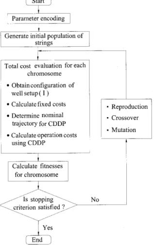
When locations of pumping wells are predetermined, the CDDP algorithm is an efficient procedure for determining optimal pump-ing rates for each well. However, the optimal pumppump-ing rates are not a complete optimization in the management model because the number of wells and locations are prespecified. In terms of the problems with fixed costs where the number of wells and loca-tions are considered as decision variables, CDDP has difficulty in solving the problem owing to the discontinuity of the fixed cost function. Therefore, this study integrates GA and CDDP to de-velop the groundwater management model defined by Eqs. 共4兲– 共8兲, as illustrated in Fig. 1. The algorithm is a simple GA with CDDP embedded in the total cost evaluation and exhibits two key features. First, the discrete nature of searching for optimal well location network alternatives is accomplished by the GA. Second, the CDDP algorithm is used to calculate optimal operating costs for time-varying pumping associated with each network

alterna-tive 共chromosome兲. These features are clarified by a sequential

explanation of the algorithm as follows: Step 0: Initialization

Encode the network alternatives as chromosomes and randomly generate an initial population. The population size in this study ranges from 50 to 100. A chromosome, I, is a binary string rep-resenting a network alternative, as indicated by Fig. 2. The length of the binary string is the total number of candidate wells. Each bit within the binary string corresponds to a candidate well. For a particular network alternative represented by a chromosome, a well is selected when the value of the corresponding bit共i兲 is one. Since the selection of wells is binary in nature, the encoding and decoding of the chromosome is straightforward. For example, the chromosome in Fig. 2 represents a network design that selects only three wells, and the well numbers are 3, 10, and 30.

Step 1: Evaluate Total Cost and Fitness Value for Each Chromosome

The chromosome described in step 0 can be represented math-ematically in the form Ik⫽x1,x2,...,xMwhere Ikdenotes a chro-mosome in the population and M is the number of total candidate wells. Since each element xl has a binary value of 1 or 0, the number of wells in this chromosome can be calculated as follows:

Nwell⫽

兺

M

xl (9)

When the number and locations of pumping wells are deter-mined, the fixed costs are readily calculated and the problem then involves evaluating the optimal operating costs for the network design. According to Eqs.共4兲–共8兲, when a network alternative is selected, the discrete and inseparable nature of the problem is eliminated and the optimization model can then be rewritten as follows: min l苸⍀ ut i ,i苸I,l⫽1,...,T J共I兲⫽

兺

再

兺

冎

repre-senting the fixed costs and does not affect the operating costs. Therefore, the CDDP can be used to evaluate the optimal operat-ing costs for the selected network design.

The CDDP algorithm exceeds conventional dynamic

program-ming共DP兲 and mathematical programming algorithms in

compu-tational efficiency共Murray and Yakowitz 1979; Jones et al. 1987兲 and does not require discretization of the state and control vector. Accordingly, CDDP overcomes the ‘‘curse of dimensionality,’’ a serious limitation for conventional DP 共Bellman and Dreyfus 1962兲. The CDDP enables a significant reduction in the ‘‘work-ing’’ dimensionality of the algorithm over that of mathematical programming algorithms by taking advantage of the dynamic na-ture of groundwater hydraulic or water quality optimization prob-lems through stagewise decomposition. On the contrary, math-ematical programming algorithms do not exploit the sequential time structure of these problems共Jones et al. 1987兲.

Fig. 1.Flowchart for groundwater management model

Fig. 2. Chromosome representation共I兲

The CDDP used herein is a procedure suggested by Murray and Yakowitz共1979兲 and is a successive approximation technique for solving optimal control problems, iteratively determining the optimal solution to the problem stated in Eq.共10兲 subject to Eqs. 共5兲–共8兲. The CDDP algorithm requires a quadratic approximation of the original problem. By substituting Eq.共5兲 into Eq. 共10兲, the objective function becomes a function of control and state vari-ables with identical time index共t兲. The second-order Taylor’s ex-pansion then approximates the objective function on the nominal policy. Since Eq.共5兲 is linear, in this study the Hessian matrix of the approximated objection function is positive definite. The ap-proximated quadratic objective function and other linear con-straints, Eqs.共6兲–共8兲, create a convex quadratic problem at every time step.

Quadratic programming in the backward and forward sweep is employed to resolve the series of quadratic problems. In the back-ward sweep, the state variables are considered as unknown pa-rameters, and the optimal control laws, which are a function of the unknown parameters, are computed. While in the forward sweep, using the initial value of state variables and the transfer function, Eq.共5兲, the value of the state variables can be specified at each time step. The quadratic programming is reapplied to solve the problem, which is moving forward, and the optimal policy is revealed. Notably, the computed optimal policy becomes the nominal policy for the next iteration. Since quadratic prob-lems are only an approximation of the original problem, iterations are required. A detailed discussion of the CDDP algorithm is pro-vided in Murray and Yakowitz共1979兲, Chang 共1986兲, Jones et al. 共1987兲, and Chang et al. 共1992兲.

After the optimal total cost J(I) for each chromosome I is calculated, the fitness for each chromosome can be evaluated as

f共I兲⫽Cmax⫺J共I兲 (11)

where Cmaxdenotes an arbitrarily large number. The procedure is

repeated for all chromosomes in each generation. Therefore, the CDDP is embedded in the GA to calculate the optimal operating costs as also indicated in Fig. 1.

Several computational issues related to the application of GA are worth mentioning. First, the capacity limitation in Eq. 共8兲 requires that the number of wells for each chromosome must be within the maximum and minimum number of wells; otherwise, no feasible solutions will be available, and the CDDP algorithm is not executed. The maximum and minimum number of wells can be determined as follows:

maximum number of wells⫽max共dt兲/umin (12) minimum number of wells⫽max共dt兲/umax (13) If the number of wells in a chromosome does not satisfy the constraints, then the fitness of this chromosome is assigned a small value.

Second, since the CDDP algorithm requires nominal policies for initialization, a systematic procedure must be developed. The nominal policies for each chromosome 共that is, network design兲 are calculated by solving a series of quadratic problems forward in time. The problems are defined as follows:

For t⫽1,...,T min ut共l兲,i傺⍀ D_tI共I兲st共I兲 (14) subject to ht⫹1⫽Fht⫹G共I兲ut共I兲⫹z, h1⫽h¯1, I艛⍀ (15) ht⫹1⭓hmin (16)

兺

u_mini ⭐u_ti共I兲⭐u_maxi ,I傺⍀ (18)

where h¯1⫽initial hydraulic heads; st(I)⫽ht⫹1(I)⫺L_*(l) ⫽vector of drawdowns. Incorporating Eq. 共15兲 into Eq. 共14兲 pro-duces a quadratic form in ui. Because Eqs.共16兲–共18兲 are linear constraints, Eqs.共14兲–共18兲 define a convex quadratic problem at each time step. Therefore, a standard quadratic programming can be used to obtain the decision variable vector. As stated previ-ously, the quadratic problems are solved independently in the for-ward direction for each time step, t. A series of decision vectors, which is a nominal policy, can then be obtained. Eq.共14兲 implies that the computed policy minimizes the drawdown and satisfies the constraints, Eqs. 共15兲–共18兲, for all stages 共time steps兲. Fur-thermore, the policy also satisfies the constraints 共5兲–共8兲 of the original problem. Therefore, if the network is designed ad-equately, the algorithm will produce a feasible solution. Other-wise, the fitness of this chromosome is assigned a small value, and the CDDP procedure is omitted. The quadratic programming technique used herein is a heuristic procedure for determining the nominal policies.

Step 2: Reproduce Best Strings

Reproduction is implemented in this study by using the roulette wheel approach. In roulette wheel reproduction, each chromo-some has the probability pj(I) of being selected.

pj共I兲⫽ fj共I兲

兺

where pop denotes the population size. This operation simulates natural selection, where a higher fitness value of a chromosome implies a higher probability that the chromosomes will survive. Therefore, the algorithm can converge to a set of chromosomes with high fitness values.

Step 3: Perform Crossover

Crossover involves random coupling of the newly reproduced strings, and each pair of strings partially exchanges information.

Fig. 3. Crossover operator

Fig. 4. Mutation operator

Crossover aims to exchange gene information so as to produce new offspring strings that preserve the best material from two parent strings. In general, the crossover occurs at a certain prob-ability ( pcross) so that it is performed on a majority of the

popu-lation. In this study, we select one point crossover as shown in Fig. 3, where pcrossranges from 0.5 to 1.0.

Step 4: Implement Mutation

Mutation restores lost or unexplored genetic material to the popu-lation to prevent the GA from prematurely converging to a local minimum. A mutation probability ( pmutat) is specified so that

ran-dom mutations can be applied to individual genes. DeJong共1975兲 originally suggested that a mutation probability inversely propor-tional to the population size would prevent the search from lock-ing onto a local optimum. This study follows DeJong’s sugges-tion. Before implementing a mutation, a random number with uniform distribution is generated. If this number is smaller than the mutation probability, then mutation is performed; otherwise, mutation is disregarded. Notably, according to the specific

prob-ability, mutation changes a specific gene共0→1 or 1→0兲 in the offspring strings produced by the crossover operation. An ex-ample of mutation is shown in Fig. 4 in the selected bit shown as the block is changed from 0 in the old string to 1 in the new string.

Step 5: Perform Termination

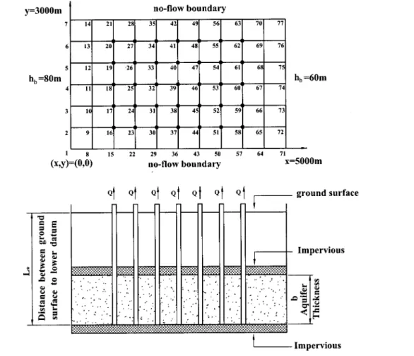
After completion of steps 1– 4, a new population is formed that requires evaluating the total cost as in step 1, which is used to assess the stopping criterion, which in turn is based on the change Fig. 5.Aquifer for water supply examples

Fig. 6. Water demand for examples and optimal pumping rates for section 4.2

Table 1. Aquifer Properties of Example Application

Parameter Value Hydraulic conductivity 4.31⫻10⫺4m/s Storage coefficient 0.001 Porosity 0.2 Aquifer thickness共b兲 50 m L * 120 m

of either the objective function value共total cost兲 or the optimized parameters. If the user-defined stopping criterion is satisfied or when the maximum allowed number of generations is achieved, the procedure terminates; otherwise, return to step 1 to perform another cycle. The success and performance of the GA depend on several parameters: the population size, number of generations, and probabilities of crossover and mutation 共McKinney and Lin 1994兲. Goldberg 共1989兲 has suggested that a good GA perfor-mance requires the choice of high-crossover and low-mutation probabilities and a moderate population size. Therefore, solutions from a GA cannot be guaranteed to be optimal. However, GAs are robust and easy to hybridize with other optimization methods or simulation models.

Numerical Results

Several example problems are presented to demonstrate the effec-tiveness of the methodology integrating a GA and CDDP. All the examples are based on the same hypothetical system as depicted in Fig. 5, adapted from Chang et al.共1992兲. Several issues related to fixed costs and constraints on individual pumping wells are considered in this demonstration. The aquifer is assumed to be homogeneous, isotropic, and confined. The 3,000⫻5,000 m site is described with 77 finite-element nodes and 35 potential well lo-cations with constant head and no-flow boundaries to circumvent the flow domain. Initial conditions on hydraulic head distribution prior to pumping are assumed to be in steady state with the aqui-fer properties listed in Table 1. In the management model, the planning horizon is divided into 36 stages over nine years. The total pumpage at each stage must satisfy the demand as shown in Fig. 6, with maximum and minimum well capacities of 0.5 and 0 or 0.01 m3/s and minimum hydraulic head of 50 m.

Three examples are examined: no fixed costs; constant unit fixed costs, and varying unit fixed costs according to geological conditions. The value of coefficient c3in these examples is set at

0.045. The performance of all examples relies on proper setting of the crossover probability ( pcross), population size, and mutation

probability ( pmutat). Numerical experiments indicate that, for pcrossin the range 0.5–1.0, population size between 50 and 100,

and pmutat⫽1/population, the computation is likely to converge to

an optimal or near-optimal solution within 22 to 43 generations. The solutions to the following examples are obtained using pcross⫽0.8 and a population size of 80 chromosomes.

Effect of Omitting Fixed Costs

The first two cases investigate the consequences of omitting fixed costs in the planning of a groundwater supply system. The value of c1is zero, and two different minimum pumping constraints on

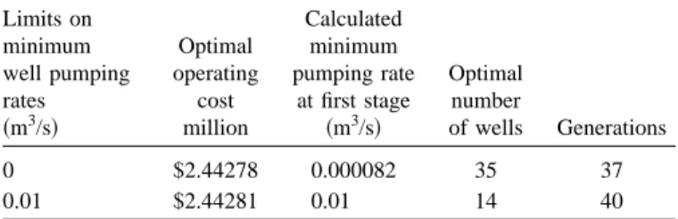
individual wells of 0 and 0.01 m3/s, respectively, are examined, with results summarized in Table 2. For the case of no fixed costs with a minimum pumping constraints of 0 m3/s, the algorithm selects all 35 candidate wells, with several wells pumping at a small rate. Since small pumping rates are infeasible for practical applications, this finding corresponds to the statement of McKin-ney and Lin共1995兲 in their study on optimal aquifer remediation. When the minimum pumping constraint is set at 0.01 m3/s, the optimal number of well installations is reduced to 14. These re-sults demonstrate that when omitting the fixed costs, the lower bound on pumpage strongly impacts the number of wells selected. However, since there are few physical or economic references, it is difficult to estimate suitable lower bounds. Fig. 7 illustrates the optimal hydraulic head distribution and pumping rates at the first time step for the case of 0.01 minimum pumping rate. Fig 8 summarizes the change of the value of the objective function and the number of wells for the optimal chromosomes in each GA generation. This simulation result indicates that solution con-verges after the 25th generation.

Fig. 7.Optimal head distribution and pumping rates at first time step for case of 0.01 minimum pumping rates共14 selected wells兲

Fig. 8. Objective function values and number of wells versus num-ber of generations

Table 2.Optimal Solutions for Different Limits on Minimum Pump-ing Rate Limits on minimum well pumping rates 共m3_/s兲 Optimal operating cost million Calculated minimum pumping rate at first stage 共m3_/s兲 Optimal number of wells Generations 0 $2.44278 0.000082 35 37 0.01 $2.44281 0.01 14 40

Table 3. Cost Comparison for Variation of Coefficient c1

Coefficient c1 $60.0 m⫺1 $120.0 m⫺1 $180.0 m⫺1 $240.0 m⫺1 Number of wells 8 7 6 5 Fixed cost共$兲 57,600 100,800 129,600 144,000 Operating cost共$兲 2,449,611 2,456,985 2,472,055 2,497,860 Total cost共$兲 2,507,211 2,557,785 2,601,655 2,641,860 CPU time共s兲 13,894 14,333 19,373 12,101

Effect of Uniform Fixed Cost on Number of Well Setup This study also considers the impact of fixed costs given a range of values of the unit fixed cost. Within each case, the unit fixed cost of each well is assumed to be the same. Constraints on the individual minimum pumping rates were relaxed 共that is, u_min

⫽0.0 m3_{/s兲 for all cases. Other constraints and the system}

con-figuration are identical to those described previously. Total fixed cost can be estimated by multiplying well depth by the unit fixed cost. The optimal value of the objective function is the optimal total cost with both the fixed and operating costs considered. Table 3 summarizes the optimal total cost, optimal number of wells, and required CPU time with respect to distinct unit fixed cost c1. These examples are calculated on a PC with an Intel

Pentium II 300 MHz CPU.

According to Table 3, increasing the unit fixed cost increases the total fixed costs, operating costs, and total cost, but decreases the total number of wells. The relationship between the optimal number of wells and the unit fixed cost resembles that between the optimal number of wells and constraints on individual mini-mum pumping rate described previously. Fig 9 plots the relation-ship between unit fixed cost, the optimal number of wells, and the minimum pumping rates at the end of the first time step

associ-ated with each optimal solution. As expected, this figure reveals that increasing the unit fixed cost increases the calculated mini-mum pumping rates and, expectedly, reduces the number of wells. The optimal head distribution at the first time step and the number and location of wells, assuming the unit fixed cost equals $180.0 m⫺1, are shown in Fig. 10. The number of wells of the optimal network is six, and the selected wells concentrate on the west side. The distribution of the location of wells is reasonable since hydraulic head is higher in the west region, thus requiring less pumping cost. Time-varying pumping rates for the six wells are shown in Fig. 6. Comparing the case of omitting fixed costs, the optimal number of wells is reduced from 14 to 6, the wells are repositioned, and the distribution of hydraulic head is altered.

Comparison of Total Cost with These Cases

The merits of considering both the fixed and operating costs are revealed by comparing the true total cost of the designed network for all cases considered. For the cases omitting fixed costs, the optimal network was determined based on only the operating costs; the operating costs are nearly the same, although the num-ber of wells differs significantly 共Table 2兲. The total cost can be estimated by adding the calculated operating costs to the fixed costs. Table 4 summarizes the total cost of the two networks given Fig. 9. Comparison of value of coefficient C1and minimum

pump-ing rate

Fig. 10. Head distribution calculated using optimal well locations, optimal number of wells, and optimal stage 1 pumping rate for each well

Table 4. Total Costs for Varying Unit Fixed Cost (c1) in Example 1

Unit fixed cost (c₁) $0 m⫺1 $60 m⫺1 $120 m⫺1 $180 m⫺1 $240 m⫺1

Lower limits共0.0 m3_/s兲 共35 wells兲 2.44 共M兲 2.69 共M兲 2.95 共M兲 3.20 共M兲 3.45 共M兲 Lower limits共0.01 m3_/s兲 共14 wells兲 2.45 共M兲 2.55 共M兲 2.65 共M兲 2.75 共M兲 2.85 共M兲

Difference of total cost ⫺0.01 共M兲 0.14 共M兲 0.30 共M兲 0.45 共M兲 0.60 共M兲

Note: M⫽million dollars.

Table 5. Comparison of Total Cost with and without Consideration of Fixed Costs in Optimization Model

Coefficient c1 $60 m⫺1 $120 m⫺1 $180 m⫺1 $240 m⫺1

Total cost and well numbers 2,507,211 2,557,785 2,601,655 2,641,860

considering fixed cost 共8 wells兲 共7 wells兲 共6 wells兲 共5 wells兲

Total cost and well numbers 2,694,780 2,946,780 3,198,780 3,450,780

considering no fixed cost 共35 wells兲 共35 wells兲 共35 wells兲 共35 wells兲

Percentage of difference共%兲 7.48 15.21 22.95 30.62

a range of unit fixed costs. Contrary to the operating costs, the two cases differ from each other significantly when the unit fixed cost is high. Table 5 compares only the total cost of the network designation.

Table 5 reveals that for the value coefficient c1as $180.0 m⫺1,

the total cost of the network for the case that does not consider fixed costs is 22.95% more than that which considers the fixed costs. This finding demonstrates the importance of considering fixed costs when the unit fixed cost is high.

Varying Unit Fixed Cost„c1…According to Geological Conditions

The last example demonstrates the capability of this procedure to solve a problem with the unit fixed cost and hydraulic conductiv-ity varying in space. Previously, the unit fixed cost and hydraulic conductivity were assumed to be the same in the study area; how-ever, this is unlikely to be true due to typical heterogeneous geo-logical conditions. Therefore, this example spatially varies the value of c1 and hydraulic conductivity to simulate the

conse-quence of geological heterogeneity. To simplify the analysis, the unit fixed costs (c1) selected are $60.0 and $180.0 m⫺1, and

hydraulic conductivity is 4.31⫻10⫺5and 4.31⫻10⫺4m/s. Figure 11 presents two geological zones and the corresponding unit fixed costs and also shows the optimal head distribution, number, and location of wells. Comparing Figs. 11共b兲 and 11共d兲 reveals that when unit fixed costs remain the same in the flow domain, the heterogeneity affects the number and location of

wells. In addition, according to Figs. 11共a and c兲 the permeability in zone II is higher than zone I, and the optimal well number increases by two. This finding indicates that a high permeability zone is desired when placing a well. More interestingly, according to Fig. 11共d兲, when unit fixed costs do not significantly differ from permeability, the latter dominates the behavior of the well setup more than the former. Table 6 lists the fixed costs, operating costs, and total costs for the four cases.

Conclusion

This study presents a novel scheme that integrates a GA with CDDP to determine the optimal solution of a groundwater man-agement problem while simultaneously considering fixed costs and time-varying operating costs. The decision variables involve the number and location of wells as well as the time-varying Fig. 11. Head distribution resulting from optimal network design and pumping scheme for first time step

Table 6.Fixed Costs, Operating Costs, and Total Costs for Examples of Varying Unit Fixed Cost (c1) According to Geological Conditions

Case

Fixed cost

共$兲 Operating cost共$兲 Total Cost共$兲

A 93,600 2,484,603 2,578,203

B 79,200 3,208,020 3,287,220

C 136,800 3,181,356 3,318,156

D 108,000 2,500,937 2,608,937

pumping rates. The number and location of wells together form a discrete optimal combinatorial problem, and the time-varying pumping rates increase the computational complexity. The pro-posed model can incorporate binary variables simply into the op-timization problem.

Simulation results demonstrate that the solution of the problem while omitting the fixed costs may be far from the true optimal network if the fixed costs are high. The fixed costs can reduce the number of wells in the network. This can also be achieved by assigning minimum pumping constraints on each well, but the appropriate pumping constraints are difficult to estimate in prac-tice without economic or physical references. Therefore, the in-clusion of fixed costs is important in the groundwater manage-ment problem, and the proposed algorithm provides a valuable reference for decision makers.

Although this study considers only groundwater supply, the proposed algorithm can be further extended to groundwater reme-diation planning. The computational loading required for the so-lution of groundwater remediation models increases with the complexity of the problem. Using the property of homogeneity of a GA can attain the speedup of convergence. That is, the chromo-some does not require further calculation when it has been calcu-lated in a previous generation of the GA. In addition, parallel implementations of the GA and the simulation model are likely to be required.

Acknowledgments

The writers would like to thank the National Science Council of the Republic of China for financially supporting this research under Contract No. NSC 88-2611-E-009-004. The writers would also like to express thanks for the useful comments of Dr. John W. Labadie, the editor, and anonymous reviewers.

References

Ahlfeld, D. P., Mulvey, J. M., and Pinder, G. F.共1988b兲. ‘‘Contaminated groundwater remediation design using simulation, optimization, and sensitivity theory, 2: Analysis of a field site.’’ Water Resour. Res., 24共5兲, 443–452.

Ahlfeld, D. P., Mulvey, J. M., Pinder, G. F., and Wood, E. F. 共1988a兲. ‘‘Contaminated groundwater remediation design using simulation, op-timization, and sensitivity theory. 1: Model development.’’ Water Re-sour. Res., 24共5兲, 431–441.

Aguado, E., and Remson, I.共1974兲. ‘‘Ground-water hydraulics in aquifer management.’’ J. Hydraul. Div., 100共1兲, 103–118.

Basagaoglu, H., and Marino, M. A.共1999兲. ‘‘Joint management of surface and ground water supplies.’’ Ground Water, 37共2兲, 214–222. Bellman, R. E., and Dreyfus, S. E.共1962兲. Applied dynamic

program-ming, Princeton University Press, Princeton, N.J.

Chang, S. C.共1986兲. ‘‘A hierarchical, temporal decomposition approach to long horizon optimal control problems,’’ PhD dissertation, Univ. of Connecticut, Storrs.

Chang, L. C., Shoemaker, C. A., and Liu, P. L. F. 共1992兲. ‘‘Optimal time-varying pumping rates for groundwater remediation: Application of a constrained optimal control algorithm.’’ Water Resour. Res., 28共12兲, 3157–3171.

Cieniawski, S. E., Eheart, J. W., and Ranjithan, S.共1995兲. ‘‘Using genetic algorithm to solve a multiobjective groundwater monitoring prob-lem.’’ Water Resour. Res., 31共2兲, 399–409.

Culver, T. B., and Shoemaker, C. A.共1992兲. ‘‘Dynamic optimal control for groundwater remediation with flexible management periods.’’

Water Resour. Res., 28共3兲, 629–641.

Culver, T. B., and Shoemaker, C. A.共1997兲. ‘‘Dynamic optimal ground-water reclamation with treatment capital costs.’’ J. Water Resour. Plan. Manage., 123共1兲, 23–29.

DeJong, K. A.共1975兲. ‘‘An analysis of the behavior of a class of genetic adaptive systems.’’ PhD dissertation, Univ. of Michigan, Ann Arbor. Goldberg, D. E.共1989兲. Genetic algorithm in search, optimization, and

machine learning, Addison-Wesley, Reading, Mass.

Gorelick, S. M.共1983兲. ‘‘A review of distributed parameter groundwater management modeling methods.’’ Water Resour. Res., 19共2兲, 305– 319.

Gorelick, S. M., Voss, C. I., Gill, P. E., Murray, W., Saunders, M. A., and Wright, M. H.共1984兲. ‘‘Aquifer reclamation design: The use of con-taminant transport simulation combined with nonlinear program-ming.’’ Water Resour. Res., 20共4兲, 415–427.

Jones, L., Willis, R., and Yeh, W. W.-G. 共1987兲. ‘‘Optimal control of nonlinear groundwater hydraulics using differential dynamic pro-gramming.’’ Water Resour. Res., 23共11兲, 2097–2106.

Lin, X., and Yang, Y.共1991兲. ‘‘The optimization of groundwater supply system in SHI JIAZ-HUANG City, China.’’ Water Sci. Technol., 24共11兲, 71–76.

McKinney, D. C., and Lin, M. D.共1994兲. ‘‘Genetic algorithm solution of groundwater management models.’’ Water Resour. Res., 30共6兲, 1897– 1906.

McKinney, D. C., and Lin, M. D. 共1995兲. ‘‘Approximate mixed-integer nonlinear programming methods for optimal aquifer remediation de-sign.’’ Water Resour. Res., 31共3兲, 731–740.

Molz, F. J., and Bell, L. C.共1977兲. ‘‘Head gradient control in aquifers used for fluid storage.’’ Water Resour. Res., 13共14兲, 795–798. Morshed, J., and Kaluarachchi, J. J. 共2000兲. ‘‘Enhancements to genetic

algorithm for optimal ground-water management.’’ J. Hydrologic Eng., 5共1兲, 67–73.

Murray, D. M., and Yakowitz, S. J. 共1979兲. ‘‘Constrained differential dynamic programming and its application to multireservoir control.’’ Water Resour. Res., 15共5兲, 1017–1027.

Murtagh, B. A., and Saunders, M. A.,共1982兲. ‘‘A projected Lagrangian algorithm and its implementation for sparse nonlinear constraints.’’ Mathematical programming study 16, North-Holland, Amsterdam, The Netherlands.

Pezeshk, S., Helweg, O. J., and Oliver, K. E.共1994兲. ‘‘Optimal operation of ground-water supply distribution systems,’’ J. Water Resour. Plng. and Mgmt., 120共5兲, 573–586.

Philbrick, C. R., and Kitanidis, P. K. 共1998兲. ‘‘Optimal conjunctive-use operations and plans,’’ Water Resour. Res., 34共5兲, 1307–1316. Pinder, G. F.共1978兲. ‘‘Galerkin finite element models for aquifer

simula-tion.’’ Rep. 78-WR-5, Dept. of Civ. Eng., Princeton Univ., Princeton, N.J.

Rosenwald, G. W., and Green, D. W.共1974兲. ‘‘A method for determining the optimum location of wells in a reservoir using mixed-integer pro-gramming.’’ Soc. Pet. Eng. J., 14共1兲, 44–54.

Taghavi, S. A., Howitt, R. E., and Marin˜o, M. A.共1994兲. ‘‘Optimal

con-trol of ground-water quality management: Nonlinear programming approach,’’ J. Water Resour. Plan. Manage., 120共6兲, 962–982. Takahashi, S., and Peralta, R. C.共1995兲. ‘‘Optimal perennial yield

plan-ning for complex nonlinear aquifers: Methods and examples,’’ Adv. Water Resour., 18共1兲, 49–62.

Wang, M., and Zheng, C.共1998兲. ‘‘Ground water management optimiza-tion using genetic algorithms and simulated annealing: Formulaoptimiza-tion and comparison.’’ J. Am. Water Resour. Ass., 34共3兲, 519–530. Wardlaw, R., and Sharif, M.共1999兲. ‘‘Evaluation of Genetic Algorithms

for Optimal Reservoir System Operation.’’ J. Water Resour. Plan. Manage., 125共1兲, 25–33.

Yeh, W. W.-G.共1992兲. ‘‘Systems analysis in ground-water planning and management.’’ J. Water Resour. Plan. Manage., 118共3兲, 224–237. Zheng, C., and Wang, P. P.共1999兲. ‘‘An integrated global and local

opti-mization approach for remediation system design.’’ Water Resour. Res., 35共1兲, 137–148.