Incomplete information analysis for the origin-destination survey table

Incomplete Information Analysis for the Origin-Destination

Survey Table

Yow-Jen Jou

; Hsun-Jung Cho

; Pei-Wei Lin

; and Chih-Yin Wang

Abstract: Sampling is one approach used to survey the origin-destination共O-D兲 trip matrix. However, when the sampling rate is not

sufficiently large compared to the population, the sampling data may have missing values in O-D pairs and that makes the O-D matrix incomplete. Two imputation methods to solve the problem mentioned previously are presented in this study. The Deming-Stephan共D-S兲 proportional fitting procedure is a statistical method first proposed to impute the missing value in this study. The improved D-S method, its convergence is proved by Cauchy criteria in this study, applies the iteration conception in the D-S method to solve the incomplete data problem. One numerical example displayed in this study shows that the improved D-S method produces an estimated O-D table with similar pattern as that of the population table.

DOI: 10.1061/共ASCE兲0733-9488共2006兲132:4共193兲

CE Database subject headings: Manufactured homes; Simulation; Models; Housing.

Introduction

To obtain the sufficient, latest, and useful trip distribution infor-mation is the fundamental and the vital task in the urban trans-portation planning study. The trip distribution data of the urban traffic can be categorized into static and dynamic categories. Dy-namic data are mainly used in short-term and middle-term traffic management and operation, whereas static data are used in long-term urban traffic planning. It is both time and budget consuming to collect the trip distribution information in traditional ways, such as lights-on survey method, license plate match method, postcard questionnaire method, and roadside interview method. In recent years, many researchers proposed estimating origin-destination共O-D兲 matrix by collecting less information to replace the traditional survey methods共Van Zuylen and Willumsen 1980; Nguyen 1984; Cascetta 1984; Spiess 1987; Bell 1991; Chang and Wu 1994; Yang et al. 1994; Hazelton 2000; Wong et al. 2005兲. The plausibility of a given O-D matrix was judged by its similar-ity to some target or prior estimate of the O-D matrix共He et al. 2002兲. Before the maturity of the estimating model developed, the survey of the trip distribution is still a vital task.

As mentioned earlier there are many traditional methods to measure the origin and destination matrix. For an open network, one of the most useful methods is the license plate match method 共Jou et al. 1996兲. When the traffic is very heavy, it is not easy to execute the population survey. The sampling survey is a proper way. However, if the sampling data are not sufficiently large, after license plate matching, the available data set becomes even smaller. In this case, some O-D pairs may have zero matching vehicles. This is called the incomplete data problem, which this study focuses to solve. In general, incomplete information can be categorized into two types: Unit nonresponse共which means that the whole information of some sampling unit is not available兲 and

Item nonresponse 共which means that some information of some

sampling unit is not available兲.

Usually, redoing the survey and replacing a reasonable value to the missing value are the two options to solve these two prob-lems. The first option is not efficient, especially when only little information is missing. The second option is a more useful and economical approach. The question is what number should be imputed to the missing cells.

To deal with this problem, one needs to understand the reason why the data are missing. Different types of missing values can be solved in different ways. Three main reasons for incomplete in-formation are listed in the following:共1兲 Missing information is caused by low demand.共2兲 The rate of sampling in every zone is small, or even zero sampling rate for some zones due to budget constraint. 共3兲 The out-of-date data may be misleading because some regions do not have travel demand in the past when unde-veloped. The first reason occurs when there is a small travel demand, and the demand might be too small to obtain when sam-pling. This paper focuses on solving incomplete information problem due to sampling.

The incomplete information problem was first noticed by Wootton共1972兲. Derbyshire 共Neffendort and Wootton 1974兲 first applied it to the practical situation. Kirby共1979兲 defined and gen-eralized the incomplete information problem. Day and Hawkins 共1979兲 applied the maximum log-likelihood approach and the trip-proportion algorithm to solve the incomplete information problem, and also calibrated the parameters and provided the

nu-1

Associate Professor, Institute of Statistics, National Chiao Tung Univ., Hsinchu, Taiwan, R.O.C. E-mail: yjjou@stat.nctu.edu.tw

2

Professor, Dept. of Transportation Technology and Management, National Chiao Tung Univ., Hsinchu, Taiwan, R.O.C. 共corresponding author兲. E-mail: hjcho@cc.nctu.edu.tw

3

Ph.D. Candidate, Dept. of Civil and Environmental Engineering, Univ. of Maryland, College Park, MD. E-mail: pwlin@wam.umd.edu

4

Student, Dept. of Transportation Technology and Management, National Chiao Tung Univ., Hsinchu, Taiwan, R.O.C. E-mail: amie.tem91@nctu.edu.tw

Note. Discussion open until May 1, 2007. Separate discussions must be submitted for individual papers. To extend the closing date by one month, a written request must be filed with the ASCE Managing Editor. The manuscript for this paper was submitted for review and possible publication on April 25, 2005; approved on December 22, 2005. This paper is part of the Journal of Urban Planning and Development, Vol. 132, No. 4, December 1, 2006. ©ASCE, ISSN 0733-9488/2006/4-193– 200/$25.00.

merical evidence. Maher共1983兲 proposed a gravity model to es-timate incomplete information problem with different perturba-tion funcperturba-tions, however, it is tough to solve this model because there were lots of uncertainties to calibrate the relevant parameters.

To classify the existing approaches, several critical issues can be summarized as follows: 共1兲 A model to produce precise esti-mate is required.共2兲 Massive computation to calibrate the model parameters is also needed. 共3兲 The information required for the model may not be easily obtained. This study, avoiding the pre-vious requirements, provides two methods to solve the incomplete information problem of the trip distribution.

The remaining sections are organized as follows. Based on the basic structure of Deming-Stephan 共D-S兲 iterative proportional fitting procedure introduced in the second section, an improved method to fit the traffic characteristics is proposed in the follow-ing section, and its convergence is theoretically proved in the section, too. To demonstrate the practical application of the two methods, two numerical examples are presented in this study. The conclusions and the future researches are proposed in the last section.

The Deming-Stephan Method

Deming-Stephan iterative proportional fitting procedure is a statistical method. To solve the incomplete information problem, requiring only the marginal values. In traffic practice, an I⫻J matrix pattern is shown in Table 1 and the notation used for model development are described as follows: Oi⫽traffic flow of the trip origin i in the network; D_j⫽traffic flow of the trip desti-nation j in the network; Tij⫽traffic flow between i and j in the network; T⫽sum of all traffic flow in the network; Tˆij⫽estimated traffic flow of the travel demand Tij in the network, such that Tˆij= Tij+ mˆij; mij⫽expected value of the travel demand Tij in the network; mˆ_ij⫽maximum likelihood estimate of m_ij in the D-S method; nˆij⫽the decimal fraction dealt with in the improved D-S method; and S⫽set of Tijs that are not zero in construction.

In Table 1, the observed value in 共i, j兲th cell is Tij, Ti+=兺jTij= Oi⫽sum of column; T+j=兺iTij= Dj⫽sum of the row, and T⫽total traffic flow. The incomplete information occurs when

some O-D pairs in cell共i, j兲 do not have value or equal to zero. This is usually caused by the sampling. This kind of incomplete information can be solved by increasing sample size, but it might not work due to the budget limit.

To accomplish a complete matrix, that is, there is no missing value in the O-D table. Let mij represent the expected value in 共i, j兲 and mijsatisfies:

The sum of column expected values

mi+=

兺

mij 共1兲

the sum of row expected values

m+j=

兺

mij 共2兲

total expected value

m++=

兺

兺

l_ij= log m_ij= u + u_1共i兲+ u_2共j兲+ u_12共ij兲 共4兲 where, u,u_1共i兲, u_2共j兲, u_12共ij兲⫽parameters; u⫽grand mean; u+u_1共i兲⫽ mean for the ith origin; u + u2共j兲⫽mean for the jth destination; and

these u items must satisfy

兺

兺

兺

兺

u =l++

IJ 共6兲

main effect of the ith origin

u_1共i兲=li+

J − l++

IJ 共7兲

main effect of the jth destination

Table 1. Example of an O-D Table

Dj Oi 1 . . . j . . . J Ti 1 T11 ¯ T1j ¯ T1J O1 ⯗ ⯗ ⯗ ⯗ ⯗ I Ti1 Tij TiJ Oi ⯗ ⯗ ⯗ ⯗ ⯗ I TI1 ¯ TIj ¯ TIJ OI Tj D1 ¯ Dj ¯ DJ T

Table 2. Degree of Freedom of u

Item u Degree of freedom

u 1

u1 I − 1

u2 J − 1

u12 IJ − I − J + 1

Sum IJ

Fig. 1. Freeway network in Example 1

u2共j兲= l+j

I + l++

IJ 共8兲

intersection between ith origin and destination

u_12共ij兲= lij−

冉

冊

The degrees of freedom of every item u is shown in Table 2. The traffic counts in a specific time interval is recorded. The vehicle arrival rate is assumed to follow the Poisson distribution. The maximum likelihood estimates of the parameters are given as follows: uˆ12共ij兲= Tij *_{− T¯} i+ * _{− T¯} +j * _{+ T¯} ++ * _共10兲 uˆ1共 兲= T¯i+ * _{− T}¯ ++ * _共11兲 uˆ2共j兲= T¯+j * _{− T¯} ++ * _共12兲 uˆ = T¯₊₊* , 共13兲 where T_ij*= log T_ij 共14兲 T ¯ i+ * ₌1 J

兺

兺

兺

兺

When N is large enough, the asymptotic distribution of uˆ12共ij兲

is a normal distribution, and the variance is共Bishop et al. 1977兲

Vˆ 共uˆ12共ij兲兲 ⬇共I − 2兲共J − 2兲_IJ

1 Tij + 1 I2 J − 2 J

兺

兺

冉

冊

兺

兺

Table 3. Freeway Origin and Destination Checklist

Origin Region Destination Region

O1 Hsinchu D1 Hsinchu O2 Hukou D2 Hukou O3 Yangmel D3 Yangmel O4 Youth D4 Youth O5 Chungli D5 Chungli O6 Neili D6 Neili O7 Airport D7 Airport O8 Taoyuan D8 Taoyuan O9 Linkou D9 Linkou

O10 Taipei D10 Taipei

O11 Yuansan D11 Yuansan

O12 Hsichih D12 Hsichih

Table 4. O-D Table of Freeway Northbound共Population兲

D O D1 D2 D3 D4 D5 D6 D7 D8 D9 D10 D11 D12 O O1 0 110 19 39 196 14 26 70 55 59 57 26 671 O2 0 20 5 8 96 7 12 41 13 13 24 7 246 O3 0 0 0 167 586 44 63 217 146 73 127 58 1,481 O4 0 0 0 0 238 20 15 116 42 31 39 21 522 O5 0 0 0 0 0 47 41 320 121 72 105 47 753 O6 0 0 0 0 0 0 4 19 10 6 4 9 52 O7 0 0 0 0 0 0 0 213 108 92 115 34 562 O8 0 0 0 0 0 0 0 0 199 133 221 60 613 O9 0 0 0 0 0 0 0 0 53 128 226 56 463 O10 0 0 0 0 0 0 0 0 0 373 2,187 476 3,036 O11 0 0 0 0 0 0 0 0 0 0 0 326 326 O12 0 0 0 0 0 0 0 0 0 0 0 0 0 D 0 130 24 214 1,116 132 161 996 747 980 3,105 1,120 8,725

Table 5. Sampling O-D Table

D O D1 D2 D3 D4 D5 D6 D7 D8 D9 D10 D11 D12 O O1 0 25 4 9 54 4 7 19 10 23 13 4 172 O2 0 5 1 0 24 0 2 11 4 4 7 3 61 O3 0 0 0 39 143 13 16 51 37 19 39 14 371 O4 0 0 0 0 54 6 2 34 10 9 12 6 133 O5 0 0 0 0 0 11 9 86 33 18 33 11 201 O6 0 0 0 0 0 0 2 4 3 2 0 3 14 O7 0 0 0 0 0 0 0 55 31 21 30 9 146 O8 0 0 0 0 0 0 0 0 48 37 61 18 164 O9 0 0 0 0 0 0 0 0 15 33 50 11 109 O10 0 0 0 0 0 0 0 0 0 93 548 120 761 O11 0 0 0 0 0 0 0 0 0 0 0 85 85 O12 0 0 0 0 0 0 0 0 0 0 0 0 0 D 0 30 5 48 275 34 38 260 191 259 793 284 2,217

Table 6. Modified O-D Matrix from Deming-Stephan Method

D O D1 D2 D3 D4 D5 D6 D7 D8 D9 D10 D11 D12 O O1 0 93 15 42 217 17 24 90 43 57 63 17 677 O2 0 25 5 9 87 3 7 40 16 12 27 9 240 O3 0 0 0 138 562 48 56 233 131 68 171 51 1,460 O4 0 0 0 0 216 21 14 119 42 30 61 21 523 O5 0 0 0 0 0 45 43 304 124 67 162 46 791 O6 0 0 0 0 0 0 6 18 10 6 7 8 55 O7 0 0 0 0 0 0 0 220 110 67 139 38 575 O8 0 0 0 0 0 0 0 0 185 121 267 72 645 O9 0 0 0 0 0 0 0 0 90 97 196 46 429 O10 0 0 0 0 0 0 0 0 0 493 2,028 474 2,995 O11 0 0 0 0 0 0 0 0 0 0 0 335 335 O12 0 0 0 0 0 0 0 0 0 0 0 0 0 D 0 118 20 189 1,082 134 150 1,023 752 1,019 3,121 1,118 8,725

兩zij兩 =

冏

冑

冏

⬎ 1.96 variables 1 and 2 are independent of each other.

The estimated values will be imputed in the incomplete cells caused by sampling. Let S⫽兵共i, j兲:Tijis not zero in construction其, then lij= log mij= u + u1共i兲+ u2共j兲+ u12共ij兲.

The model parameters, u, must satisfy the following constrains:

兺

兺

兺

兺

再

再

再

If Tijfollows a Poisson distribution, the likelihood function of mij is

兿

mˆ_ij= T¯ij 共25兲

However, it is difficult to obtain the average value of the trip distribution. To deal with this problem, the following assumptions are proposed:

Table 7. Modified O-D Matrix from Improved Deming-Stephan Method

D O D1 D2 D3 D4 D5 D6 D7 D8 D9 D10 D11 D12 O O1 0 98 16 35 212 16 28 75 39 90 51 16 676 O2 0 20 4 3 94 2 8 43 16 16 28 12 245 O3 0 0 0 153 562 51 63 201 145 75 153 55 1,459 O4 0 0 0 0 212 24 8 134 39 35 47 24 523 O5 0 0 0 0 0 43 35 338 130 71 130 43 790 O6 0 0 0 0 0 0 8 16 12 8 4 12 59 O7 0 0 0 0 0 0 0 216 122 83 118 35 574 O8 0 0 0 0 0 0 0 0 189 145 240 71 645 O9 0 0 0 0 0 0 0 0 59 130 197 43 429 O10 0 0 0 0 0 0 0 0 0 366 2,155 472 2,992 O11 0 0 0 0 0 0 0 0 0 0 0 334 334 O12 0 0 0 0 0 0 0 0 0 0 0 0 0 D 0 118 20 191 1,081 136 149 1,022 751 1,018 3,121 1,117 8,725

Fig. 2. Distribution of the estimation results

mˆ_i+= Ti+, i = 1, . . . ,I 共26兲 mˆ_+j= T_+j, j = 1, . . . ,J 共27兲

The following is the estimation algorithm, which estimates the missing value mijiteratively:

Step 0—set mˆ_ij共0兲=␦ij, ∀ i, j 共28兲 Step V—compute the following equations iteratively until the criterion:兩mˆ_ij共2V−1兲− mˆ_ij共2V兲_{兩 ⬍␧ is satisfied, where}

mˆ_ij共2V−1兲= mˆij 共2V−2兲_T i+

兺

兺

The purpose of the D-S method is to solve the incomplete information occurs in the general questionnaire. If D-S iterative

proportional fitting procedure is employed directly in O-D matri-ces, the results may not be accurate since the imputed values would be incorrectly large in structure.

The Improved Deming-Stephan Method

The idea of the improved D-S method is that when Oiand Djare large, Tijwill be relatively large. Other ideas follow the structure of the D-S iterative proportional fitting procedure.

Table 8. ERR from Both Methods

Method

ERR 共%兲

Sample amplified directly 6.596

Deming-Stephan method 11.114

Improved Deming-Stephan method 6.524

Table 9. Matrix of Trips between Each Node Pair共Thousand of Vehicles/Day兲 共Sample兲

D O D1 D2 D3 D4 D5 D6 D7 D8 D9 D10 D11 D12 D13 D14 D15 D16 D17 D18 D19 D20 D21 D22 D23 D24 D1 0 2 2 6 3 4 51 9 6 14 6 3 6 4 6 6 5 2 4 4 2 5 4 2 D2 2 0 2 3 2 5 3 5 3 7 3 2 4 2 2 5 3 0 2 2 0 2 0 0 D3 2 2 0 3 2 4 2 3 2 4 4 3 2 2 2 3 2 0 0 0 0 2 2 0 D4 6 3 3 0 6 5 5 8 8 13 15 7 7 6 6 4 6 2 3 4 3 5 6 3 D5 3 2 2 6 0 3 3 6 9 11 6 3 3 2 3 6 3 0 2 2 2 3 2 0 D6 4 5 4 5 3 0 5 9 5 9 5 3 3 2 3 10 6 2 3 4 2 3 2 2 D7 6 3 2 5 3 5 0 11 7 20 6 8 5 3 6 15 11 3 5 6 3 6 3 2 D8 9 5 3 8 6 9 11 0 9 17 9 7 7 5 7 23 15 4 8 10 5 6 4 3 D9 6 3 2 8 9 5 7 9 0 29 15 7 7 7 10 15 10 3 5 7 4 8 6 3 D10 14 7 4 13 11 9 20 17 29 0 41 21 20 22 41 45 40 8 19 26 13 27 19 9 D11 6 3 4 16 6 5 6 9 15 40 0 15 11 17 15 15 11 2 5 7 5 12 14 7 D12 3 2 3 7 3 3 8 7 7 21 15 0 14 8 8 8 7 3 4 5 4 8 8 6 D13 6 4 2 7 3 3 5 7 7 20 11 14 0 7 8 7 6 2 4 7 7 14 9 9 D14 4 2 2 6 2 2 3 5 7 22 17 8 7 0 14 8 8 2 4 6 5 13 12 5 D15 6 2 2 6 3 3 6 7 11 41 15 8 8 19 0 13 16 3 9 12 9 27 11 5 D16 6 5 3 9 6 10 15 23 15 45 15 8 7 8 13 0 29 6 14 17 7 13 6 4 D17 5 3 2 6 3 6 11 15 10 40 11 7 6 8 16 29 0 7 18 18 7 18 7 4 D18 2 0 0 2 0 2 3 4 3 8 3 3 2 2 3 6 7 0 4 5 2 4 2 0 D19 4 2 0 3 2 3 5 8 5 19 5 4 4 4 9 14 18 4 0 13 5 13 4 2 D20 4 2 0 4 2 4 6 10 7 26 7 6 7 6 12 17 18 5 13 0 13 25 8 5 D21 2 0 0 3 2 2 3 5 4 13 5 4 7 5 9 7 7 2 5 13 0 19 8 6 D22 5 2 2 5 3 3 6 6 8 27 12 8 14 13 27 13 18 4 13 25 19 0 22 12 D23 4 0 2 6 2 2 3 4 6 19 14 8 9 12 11 6 7 2 4 8 8 22 0 8 D24 2 0 0 3 0 2 2 3 3 9 7 6 8 5 5 4 4 0 2 5 6 12 8 0

Fig. 3. Network in Example 2

Table 10. Matrix of Trips between Each Node Pair共Thousand of Vehicles/Day兲 共D-S method兲 D O D1 D2 D3 D4 D5 D6 D7 D8 D9 D10 D11 D12 D13 D14 D15 D16 D17 D18 D19 D20 D21 D22 D23 D24 D1 0 2.420 1.991 9.236 4.178 5.725 56.029 14.144 10.988 31.311 13.384 7.109 10.302 8.331 12.961 14.697 12.788 2.672 7.656 9.806 4.981 13.193 8.301 3.797 D2 1.951 0 1.294 3.257 1.646 4.809 3.789 5.823 3.777 11.434 4.488 2.516 4.573 2.582 3.363 6.878 4.608 0.496 2.382 3.020 1.181 3.728 1.573 0.830 D3 1.664 1.294 0 2.877 1.451 3.564 2.248 3.272 2.240 6.792 4.736 3.058 2.098 2.104 2.649 4.008 2.820 0.346 0.964 1.409 0.824 2.904 2.098 0.579 D4 7.695 3.194 2.833 0 6.832 6.292 9.071 12.168 12.037 27.402 21.052 10.297 10.460 9.484 11.696 11.156 12.392 2.407 5.916 8.725 5.348 11.732 9.458 4.353 D5 3.458 1.646 1.451 6.928 0 3.240 4.744 7.797 10.726 18.334 8.816 4.325 4.413 3.426 5.623 9.413 6.000 0.761 3.119 4.098 2.812 6.184 3.412 1.273 D6 4.824 4.809 3.564 6.412 3.240 0 7.433 11.498 7.410 18.426 8.773 4.909 5.019 4.035 6.533 14.521 10.004 1.952 4.651 6.875 3.267 7.234 4.018 2.593 D7 7.978 3.320 1.921 7.937 4.024 6.533 0 15.711 11.566 36.021 12.793 11.749 8.928 6.955 12.400 23.013 18.169 3.554 8.328 11.327 5.700 13.545 6.927 3.600 D8 12.114 5.823 3.272 12.439 7.797 11.498 17.741 0 15.689 39.512 18.765 12.560 12.808 10.845 16.222 34.451 25.284 5.147 12.979 17.739 9.112 16.804 9.806 5.592 D9 8.986 3.767 2.233 12.270 10.710 7.390 13.501 15.644 0 50.781 24.430 12.356 12.596 12.632 18.904 26.064 19.933 4.080 9.793 14.468 7.953 18.437 11.594 5.480 D10 25.285 11.445 6.799 28.240 18.350 18.446 42.115 39.557 50.959 0 72.143 39.587 39.328 41.440 70.522 81.178 72.693 13.411 35.852 51.095 27.263 61.245 38.322 18.724 D11 10.590 4.478 4.729 22.390 8.800 8.753 15.518 18.720 24.448 70.947 0 22.913 19.250 25.301 27.889 30.917 25.332 3.917 12.123 17.875 10.945 27.038 22.247 10.880 D12 5.397 2.506 3.051 10.491 4.309 4.889 13.392 12.515 12.349 39.416 22.889 0 18.622 12.653 15.441 17.282 15.318 3.773 7.937 11.217 7.221 16.747 12.620 7.966 D13 8.574 4.584 2.105 10.724 4.429 5.039 10.724 12.853 12.679 39.423 19.351 18.698 0 11.946 15.879 16.815 14.802 2.865 8.193 13.591 10.440 23.253 13.912 11.120 D14 6.452 2.530 2.068 9.563 3.346 3.935 8.495 10.620 12.452 40.728 25.032 12.504 11.712 0 21.577 17.447 16.468 2.802 8.016 12.333 8.289 21.904 16.711 7.014 D15 10.472 3.425 2.692 12.233 5.719 6.653 15.296 16.493 20.226 71.270 28.317 15.724 16.054 27.104 0 28.559 30.007 4.856 15.951 22.623 14.798 41.699 19.052 8.777 D16 11.611 6.930 4.044 16.739 9.493 14.621 26.438 34.677 26.355 81.779 31.296 17.540 16.939 17.999 28.424 0 46.131 8.450 22.606 30.042 14.213 30.966 15.936 8.771 D17 9.885 4.608 2.820 12.779 6.000 10.004 21.072 25.284 19.998 72.629 25.397 15.383 14.737 16.791 29.620 45.808 0 9.071 25.551 29.500 13.311 33.883 15.734 8.137 D18 2.143 0.507 0.354 2.511 0.777 1.972 4.151 5.192 4.137 13.533 4.991 3.823 2.892 2.902 4.840 8.460 9.136 0 4.661 6.428 2.420 6.280 2.891 0.998 D19 6.118 2.382 0.964 6.121 3.119 4.651 9.866 12.979 9.827 35.818 12.157 7.971 8.159 8.187 15.746 22.435 25.551 4.627 0 18.623 7.874 20.945 8.158 3.722 D20 7.581 3.030 1.417 9.056 4.114 6.895 13.620 17.785 14.562 51.180 17.986 12.304 13.580 12.622 22.382 29.864 29.564 6.391 18.657 0 17.692 37.143 14.578 7.999 D21 3.666 1.181 0.824 5.524 2.812 3.267 7.016 9.112 7.982 27.234 10.975 7.250 10.411 8.435 14.623 14.067 13.311 2.391 7.874 17.662 0 25.648 11.410 7.327 D22 10.156 3.728 2.904 12.137 6.184 7.234 16.582 16.804 18.504 61.178 27.106 16.815 23.186 22.242 41.294 30.629 33.883 6.212 20.945 37.076 25.648 0 31.183 16.373 D23 6.549 1.573 2.098 9.692 3.412 4.018 8.678 9.806 11.633 38.283 22.286 12.659 13.873 16.905 18.818 15.741 15.734 2.852 8.158 14.539 11.410 31.183 0 10.098 D24 2.849 0.820 0.572 4.445 1.257 2.573 4.480 5.546 5.456 18.569 10.839 7.949 10.060 7.077 8.595 8.597 8.072 0.965 3.687 7.928 7.298 16.306 10.059 0 198 / JOURNAL OF URBAN PLANNING AND DEVELOPMENT © ASCE / DECEMBER 2006

When a zero sampled value occurred for a structural nonzero

T_ij, we impute a fraction by the following algorithm and then amplify the imputed data by the population size:

Step 0—set nˆ_ij共0兲=␦ij, ∀ i 共31兲

Step V—compute the following equations iteratively until the cri-terion:兩nˆ_ij共2V−1兲− nˆ_ij共2V兲兩 ⬍␧ is satisfied, where

nˆ_ij共2V−1兲=

冉

冊

冉

冊

where Oi and Dj⫽represented as number of trips, and,

关nˆij 共2V−2兲_/共nˆ ij 共2V−2兲_{+ O} i兲兴 and 关nˆij 共2V−1兲_/共nˆ ij 共2V−1兲_{+ D} j兲兴 are fractions, so nˆij can certainly stand for the number of trips. nˆij is positively related to Oi and Dj, so the model fits the positive proportion assumption.

If the sequence 关nˆij兴 is convergent, then the sequence exists and can imply to the practice.

• Definition: If∀␧⬎0, and there exists a natural number N let

兩nˆ_ij共2V−1兲_{− nˆ} ij

共2V兲_{兩 ⬍␧ when 2V−1,2VⱖN. Then the sequence}

关nˆij兴 is called Cauchy sequence.

• Theorem:共Cauchy convergence criterion兲 The sequence 关nˆij兴

is convergent if and only if the sequence is Cauchy sequence.

• Proof:兩nˆ_ij共2V−1兲− nˆ_ij共2V兲兩 ⬍␧ when ∀共i, j兲苸S, ␧⬎0.

Take N as a natural number and let n_ij共2N−1兲⬍共␧/2兲+

冑

冉

冊

冉

冊

冑

冑

冑

冑

Therefore, sequence关nˆij兴 is Cauchy sequence. And according to Cauchy convergence criterion, sequence关nˆ_ij兴 converges.

Empirical Example

This research has developed a model to solve the incomplete information problem caused by sampling. Two numerical ex-amples are demonstrated to show the practical application of the proposed model.

Example 1

The data of example 1 are collected from the freeway northbound as shown in Fig. 1. The survey time is from 6:30 to 10:30 in the morning on 14th December in 1994. Table 3 is the list of all of the origins and destinations.

Table 11. Matrix of Trips between Each Node Pair共Thousand of Vehicles/Day兲 共Improved D-S method兲

D O D1 D2 D3 D4 D5 D6 D7 D8 D9 D10 D11 D12 D13 D14 D15 D16 D17 D18 D19 D20 D21 D22 D23 D24 D1 0 2 2 6 3 4 51 9 6 14 6 3 6 4 6 6 5 2 4 4 2 5 4 2 D2 2 0 2 3 2 5 3 5 3 7 3 2 4 2 2 5 3 0.068 2 2 0.105 2 0.120 0.088 D3 2 2 0 3 2 4 2 3 2 4 4 3 2 2 2 3 2 0.068 0.113 0.136 0.105 2 2 0.088 D4 6 3 3 0 6 5 5 8 8 13 15 7 7 6 6 4 6 2 3 4 3 5 6 3 D5 3 2 2 6 0 3 3 6 9 11 6 3 3 2 3 6 3 0.069 2 2 2 3 2 0.088 D6 4 5 4 5 3 0 5 9 5 9 5 3 3 2 3 10 6 2 3 4 2 3 2 2 D7 6 3 2 5 3 5 0 11 7 20 6 8 5 3 6 15 11 3 5 6 3 6 3 2 D8 9 5 3 8 6 9 11 0 9 17 9 7 7 5 7 23 15 4 8 10 5 6 4 3 D9 6 3 2 8 9 5 7 9 0 29 15 7 7 7 10 15 10 3 5 7 4 8 6 3 D10 14 7 4 13 11 9 20 17 29 0 41 21 20 22 41 45 40 8 19 26 13 27 19 9 D11 6 3 4 16 6 5 6 9 15 40 0 15 11 17 15 15 11 2 5 7 5 12 14 7 D12 3 2 3 7 3 3 8 7 7 21 15 0 14 8 8 8 7 3 4 5 4 8 8 6 D13 6 4 2 7 3 3 5 7 7 20 11 14 0 7 8 7 6 2 4 7 7 14 9 9 D14 4 2 2 6 2 2 3 5 7 22 17 8 7 0 14 8 8 2 4 6 5 13 12 5 D15 6 2 2 6 3 3 6 7 11 41 15 8 8 19 0 13 16 3 9 12 9 27 11 5 D16 6 5 3 9 6 10 15 23 15 45 15 8 7 8 13 0 29 6 14 17 7 13 6 4 D17 5 3 2 6 3 6 11 15 10 40 11 7 6 8 16 29 0 7 18 18 7 18 7 4 D18 2 0.063 0.053 2 0.078 2 3 4 3 8 3 3 2 2 3 6 7 0 4 5 2 4 2 0.088 D19 4 2 0.053 3 2 3 5 8 5 19 5 4 4 4 9 14 18 4 0 13 5 13 4 2 D20 4 2 0.053 4 2 4 6 10 7 26 7 6 7 6 12 17 18 5 13 0 13 25 8 5 D21 2 0.063 0.053 3 2 2 3 5 4 13 5 4 7 5 9 7 7 2 5 13 0 19 8 6 D22 5 2 2 5 3 3 6 6 8 27 12 8 14 13 27 13 18 4 13 25 19 0 22 12 D23 4 0.063 2 6 2 2 3 4 6 19 14 8 9 12 11 6 7 2 4 8 8 22 0 8 D24 2 0.063 0.053 3 0.078 2 2 3 3 9 7 6 8 5 5 4 4 0.068 2 5 6 12 8 0

A vehicle is a matched license plate if its plate number, includ-ing two English letters and four digits, can be found from one on-ramp and off-ramp. To allow minor coding error, plate num-bers with only one different code are considered as a match. The license plates which can be found only from either one on-ramp or one off-ramp are eliminated. Table 4 shows the O-D matrix after matching. Table 5 is the example matrix sampling from Table 4. The sampling matrix is sampled every two vehicles, e.g., 1 , 3 , 5 , 7 , . . ., and so on.

Tables 6 and 7 show the O-D matrix modified and magnified by Deming-Stephan iterative proportional fitting procedure and the improved Deming-Stephan method, respectively. Fig. 2 illus-trates the distribution of population O-D and estimated O-D. Table 8 summarizes the estimation error, which is defined as follows:

ERR =

兺

兺

⫻ 100% 共34兲

where Tij⫽O-D trip of population and Tˆij⫽The sampling data

after modeling process and magnifying

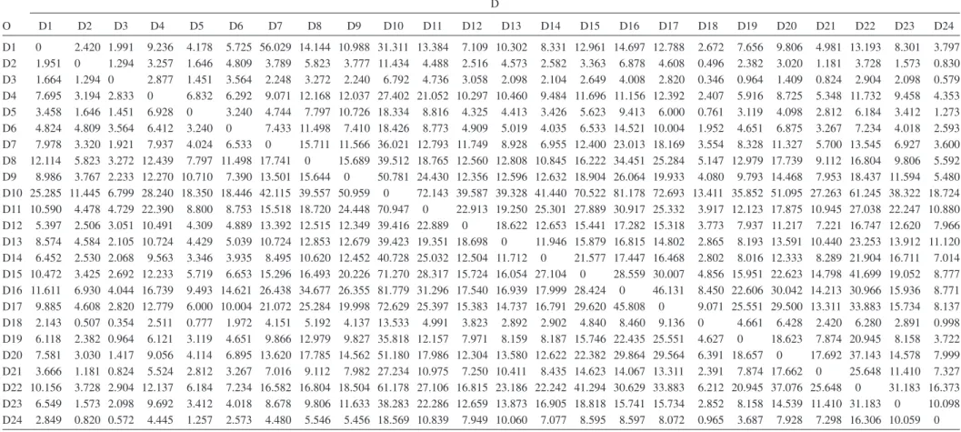
Example 2

Fig. 3 is a network used to model city of Sioux Falls, S.D. Each node was considered an origin and destination, and there are 24 nodes in the network. And the matrix of demands for trips be-tween the nodes is given in Table 9. 共LeBlanc 1985兲 There are some nonstructure zeros existing in the O-D matrix. Table 10 and Table 11 are the demands for trips between the nodes imputed by the Deming-Stephan method and improved D-S method, respectively.

Conclusions

In this paper, we presented two imputation methods, the Deming-Stephan method and the improved one, to solve incomplete O-D matrix problems. And the two methods perform well under the assumption that Tij’s obey the Poisson distribution only.

Example results show that, although the amplified-directly sample has smaller ERR than the D-S method, the missing cells are still missing. Both the D-S method and the improved one can impute the missing values. And the improved D-S method has been proven to perform much better than the D-S method.

Here is some further research. Multiple values can be imputed into the missing cells to account for the valuation in the imputed values.

Acknowledgments

This research was partially supported by the Ministry of Educa-tion, Taiwan, R.O.C., under Grant No. EX-91-E-FA06-4-4 and

partially supported by National Science Council of Taiwan, R.O.C., under Grant Nos. 2218-E-009-042 and NSC-93-2218-E-009-043.

References

Bell, M. G. H.共1991兲. “The estimation of origin–destination matrices by constrained generalized least squares.” Transp. Res., Part B: Meth-odol., 23, 257–265.

Bishop, Y. M. M., Feinberg, S. E., and Holland, P. W.共1977兲. Discrete multivariate analysis: Theory and practice, MIT Press, Cambridge, Mass.

Cascetta, E.,共1984兲. “Estimation of trip matrices from traffic counts and survey data: A generalized least squares estimator.” Transp. Res., Part B: Methodol., 18, 289–299.

Chang, G. L., and Wu, J.共1994兲. “Recursive estimation of time-varying flows from traffic counts in freeway corridors.” Transp. Res., Part B: Methodol., 28, 141–160.

Day, M. J. L., and Hawkins, A. F.共1979兲. “Partial matrices, empirical deterrence functions and ill-defined results.” Traffic Eng. Control, 429–433.

Hazelton, M. L.共2000兲. “Estimation of origin-destination matrices from link flows on uncongested networks.” Transp. Res., Part B: Meth-odol., 34, 549–566.

He, R. R., Kornhauser, A. L., and Ran, B.共2002兲. “Estimation of time-dependent O-D demand and route choice from link flows.” Proc., 81st Transportation Research Board Annual Meeting, Washington, D.C. Jou, Y.-J., Cho, H.-J., and Lee, H. 共1996兲. “The study of

origin-destination sampling survey in highway and incomplete data analy-sis.” Transportation Planning Journal, 25共4兲, 709–726.

Kirby, H. R.共1979兲. “Partial matrix techniques.” Traffic Eng. Control, 424–428.

LeBlanc, L. J. 共1985兲. “An algorithm for the discrete network design problem.” Transp. Sci., 9共3兲, 183–199.

Maher, M. J. 共1983兲. “The use of prior information on gravity model calibration.” Traffic Eng. Control, 68–72.

Neffendort, H., and Wootton, H. J.共1974兲. “A travel estimation model based on screen-line interviews.” Proc., PTRC Summer Annual Meet-ing, Univ. of Warwick Seminar N: Urban traffic models, Planning and Transport Research and Computation Co. Ltd., London.

Nguyen, S.共1984兲. “Estimation of origin–destination matrices from ob-served flows.” Transportation Planning Models, 363–380.

Spiess, H.共1987兲. “A maximum likelihood model for estimating origin-destination matrices.” Transp. Res., Part B: Methodol., 21, 395–412. Wong, S. C., et al.共2005兲. “Estimation of multiclass origin-destination matrices from traffic counts.” J. Urban Plann. Dev., 131共1兲, 19–29. Wootton, H. J.共1972兲. “Calibration a gravity model and estimating trip

ends from a partially observed trip matrix.” Memorandum of Decem-ber 21.

Yang, H., Iida, Y., and Sasaki, T.共1994兲. “The equilibrium-based origin-destination matrix estimation problem.” Transp. Res., Part B: Meth-odol., 28, 23–33.

Van Zuylen, J. H., and Willumsen, L. G.共1980兲. “The most likely trip matrix estimated from traffic counts.” Transp. Res., Part B: Meth-odol., 14, 281–293.