Copyright 0 1996 Elsevier Science Ltd Printed in Great Britain. All rights reserved
0097-8493/96 $15.00+0.00 PII: soo97-8493(~3
Technical Section
RWM-CUT
FOR COLOR
IMAGE
QUANTIZATION
CHING-YUNG YANG and JA-CHEN LINt
Institute of Computer and Information Science, National Chiao Tung University, Hsinchu, Taiwan 300, R.0.C
e-mail: jclin@,cis.nctu.edu.tw
A new simple method for constructing a color palette that uses the radius weighted mean cut (RWM-cut) is proposed. The method is a hierarchically divisive method, and each two-class partition uses the centroid and the RWM only. Experiments show that the RWM-cut algorithm is feasible and visually acceptable. The algorithm can either be used alone or be used to create a good initial palette for the LBG algorithm. Besides the 3-D version, a 1-D version of the RWM-cut algorithm is also included in the paper for real- time color quantization. The quantization error is small and the processing speed is competitive. Dithered images are also provided. Copyright 0 1996 Elsevier Science Ltd
1. INTRODUCTION
The process of reproducing a color image using a very limited number of colors suitably generated from that given image is called color quantization. In general, people quantize a full-color (typically 16 million colors) image into one with 256 (or fewer than 256) colors. A full-color image can then be displayed directly on commonly used output devices such as the monitor of a low-cost workstation or PC. The other application of color quantization is that: when a color image is to be compressed, the compression ratio can often become higher if the compression technique is combined with color quantization using, say, 64 colors only. Roughly speaking, color quantization includes two parts: the generation of an appropriate palette, and the correspondence that assigns to each input pixel one of the palette colors. Since the size of the palette is quite limited, it is critical to derive a good palette. The designer, when the palette size is fixed, should try to make the perceived quality of the reproduced image as close as possible to the original one [l].
A number of approaches [l-9] have been proposed to perform color image quantization. The LBG algorithm developed by Linde et al. [2] is a simple method that is easy to implement, but it has the following drawbacks: a poorly selected initial palette may lead to an undesirable 6nal palette, and a complete design requires a large number of computa- tions. Heckbert [3] proposed the mediancut algo- rithm for color quantization. The algorithm recursively divided the reduced (S-5-5) RGB color space (that is, the 24 bit image is 6rst reduced to a 15 bit image in a pre-processing via discarding the three least significant bits for each RGB component)
+ Author for correspondence.
into two subboxes containing approximately equal number of colors until the desired number of subboxes is reached. Finally, the color palette is formed by collecting the centroids of these subboxes. Although the algorithm is simple, a greater visible distortion exists in the quantized image. Kurz [4] presented another simple algorithm called the uni- form quantization algorithm to quantize colors. The principle of the algorithm is that the 3-D color space is divided into N rectangular subboxes of equal size. Then, the centers of these subboxes are used as the N representative colors. In spite of the simplicity of the uniform quantization technique, false contours severely exhibit in the quantized images, especially when the size of the palette is less than 256. Wu and Witten [5] suggested the mean-split algorithm. The hyperplane they used for partition passes through the mean of the longest projected data component. Since it is simpler to compute the mean than to compute the median, the processing speed of the mean-split algorithm is faster than that of the median-cut algorithm. However, a partition plane passing through the mean instead of the median does not necessarily result in lower quantization error [6]. Wan et al. therefore proposed an elegant method called the variance-based algorithm [l] to quantize colors based on the goal of minimizing the sum of squared error. The idea of that algorithm is to sweep a cutting plane along a direction parallel to one of the reduced RGB coordinate axes, and then split the current box at the position where the sum of squared “1-D” error (defined in equation (11) of [l]) of the projected distribution in the corresponding axis is minimized. Since the algorithm is specifically designed by inspecting the sum of squared error from time to time, the algorithm can often produce a quantized image whose sum of squared “3-D” error, which is the right hand side of our Eq. (1) given at the end of this section (without the denominator), is low (but 517
578 C.-Y. Yang and J.-C. Lin not minimal). Unfortunately, the computation com-
plexity is not attractive. (The computation complex- ity would have been even higher if they had tried to cut along one of the coordinate axes at the position where the sum of “3-D” error is minimized.) Orchard and Bouman [7] presented a delicate algorithm for the design of a treestructured color palette incorpor- ating a performance criterion which reflects the subjective evaluation of image quality. Although the algorithm results in images with small artifacts, the implementation of the algorithm is not very simple, because the computation for the principal axis is required each time a node is split during the construction of the color palette. Wu [8] used the dynamic programming technique to derive a nearly optimal color palette. The basic idea of the algorithm is to simultaneously optimize K-l cuts along the principal axis if K colors are desired. This partition strategy leads to small quantization error. However, the time complexity of the algorithm is a problem. For example, it may take about 3 min on a personal IRIS workstation to quantize a full-color image into one with 256 colors. This method is therefore not suitable for the applications in which the processing speed is of big concern. A method faster than Wu’s dynamic programming technique is the center-cut algorithm [9] proposed by Joy and Xiang who made three modifications to the median-cut method. The three modifications are (1) to utilize 5-6-4 instead of 5-S-5 color reduction for each RGB pixel; (2) to partition the color box whose longest-dimension is the longest among all boxes (explained in [9]) instead of partitioning the color box whose pixel count is the largest; and (3) to cut through the center of the color box instead of bisecting the box’s pixel count. Basically, the center-cut algorithm inherits the advantages of the median-cut method and improves the performance of that technique. However, the distortion of the color hue introduced by the center- cut algorithm is severe.
representative color of the palette.) A major reason for adopting the nearest neighbor rule is that the mean-squared error (MSE) of the quantized images can be minimized by mapping each pixel to the palette color that is closest to it. The MSE is defined as
From the above analysis, we can see that the existing algorithms often become computationally inconvenient or yield unsatisfactory quantization error. In this paper, we develop a new simple method for color palette generation. The method can work well if it is used alone; on the other hand, it can also be used to initialize and accelerate the LBG algorithm. In the new method, we employ the radius weighted mean (RWM), a special kind of point originally introduced to register shapes [lo, 111. We refer to our method as the RWM-cut method, which is a hierarchically divisive method [12], and will be described in detail in the next section. Once the palette is created, each color pixel can then be reproduced by finding the nearest neighbor of the color in the palette, if processing time is not of big concern. (For real-time applications, however, a faster way to do color mapping is that: at the final step of a K-color palette-generating procedure, just map all color pixels in color box j (15 j 5 K) to the centroid of these color pixels, i.e. to the jth
MSE = iii
if the image size is M x N. Here, P and P’ denote the 3-D color values of the input image and the quantized image, respectively.
The remaining part of the paper is organized as follows. The proposed RWM-cut algorithm for deriving a color palette is described in Section 2. In Section 3, the RWM-cut algorithm is first used alone. Then, the LBG algorithm with initial palette generated by different methods are discussed. In Section 4, we compare the real-time simulations obtained from various algorithms, including the RWM-cut, median-cut, mean-split, center-cut, and variance-based algorithms. Examples of applying the spatial dithering to the quantized images generated by the proposed RWM-cut algorithm are also provided there. The summary of the paper is given in Section 5.
2. THE RWM-CUT ALGORlTHM
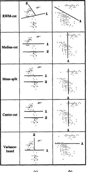
Before giving the formal definition of the RWM- cut algorithm, which can handle data of any dimension, we first show the good partition ability of the RWM-cut. The examples are 2-D becausethey are easier to illustrate. The data listed in Fig. I(a and b) are, respectively, the 2-D projection of the quite famous 87-point Chernoff Fossil data and 150-point Fisher Iris data commonly used as the test data in the field of data analysis [13]. We can see that the RWM- cut partitions the data better than the median-cut, mean-split, and center-cut do. As for the variance- based algorithm, although its partition result is competitive with that of the RWM-cut in Fig. 1, its computation speed is slower than that of the RWM- cut. The performance of the partition results are summarized in Table 1. It can be seen that the RWM- cut algorithm obtains a smaller total sum of squared error (TSSE) than the other algorithms do, and the computation speed of the RWM-cut algorithm is also not bad. Note that the TSSE (of a K-cluster partition), which is the sum of the squared Euclidean distances between each data point and its cluster mean is defined by
TSSE = 2 c 11x - m# (4 j=l xeCj
Also note that x is the data point belong&g to cluster C,, and mj is the centroid of the cluster C’: The error represents the accumulated deviations~from the
RWM-cut all . . .2 ..” : ‘i :.. . I . ‘>” . 1 ::..: . - ” .>w . :..:::.: :. .‘A. : ... . ..a. fled&cut -“’ .“. 1 . “:.” . . . . :::: ::.. . . . . . i ::’ .’ i’ 2 i :. : ..>‘* . . :‘.: . 1 ..- .:,,* ..,C. 9.v.. ..:..:::.: :. ” . ” 1 : **. Mesa-split . . . . “:.” . . .- 2 . .*::. *. . :::: ::.. .:> c . 1.. . ; .: .:. * .: :.. . : . 1 Center-cut *:;< a\<* . :..:::.: :. . ..a . * .- ... . . . . 1 * “:.” . . . . . ..I . . . *. . . :I::.::.* ‘;“.” 2 : *: : . . . . . . .:. +::. > . . ‘:‘.: . : 1 2 ,i:..:.:.: :. . . . . . ..- .:v ’ 1 . .:+I”. . . . . 1 “sriance . . . . based -“’ . . . .y::;:... 1 i :‘**” : :. . : ‘.$.. . : :.. . : . . . 2’” (4 CJ)
Fig. 1. The resulting clusters generated by different methods. Each row corresponds to a method; each column corre- sponds to a data set; each straight line i (i= 1,2) corresponds
to the ith partition boundary.
data points to the centroids. In other words, the smaller the TSSE, the better the partition result. We also point out here that, as stated in the second paragraph of the introduction section, the variance- based algorithm cannot guarantee the smallest (2-D) TSSE although its cutting point is at the position where the sum of squared “1-D” error is minimized. [In Fig. l(b), the variance-based algorithm only minimizes c(x,y)eA lY-~~l++(,,y)eBIY-~El.
Here, jj~ and j$ are the means of the y coordinate of the two resulting 2-D subclasses A and B, respectively.]
We discuss below the procedure that we will use to partition data. To make the reading easier, two examples are provided to illustrate the procedure. Although the examples shown here are 2-D, the reader can still get the idea how the algorithm proceeds, and then extend the idea to the 3-D case. Note that when the data are 2-D, say,
s = {(x. y.)}!!
I, I
I lj the centroid 0 iswhereas the RWM R (defined by Mitiche and Aggarwal [IO]) is C WiXi C WYi (2, y’) = i n-&l i i with Wi = d(Xi - 2)’ + bi - Y)*
being the distance between the centroid and the ith data point. The boundary that we proposed to partition the 2-D data set S into two subsets is then taken to be the line through R and perpendicular to oft.
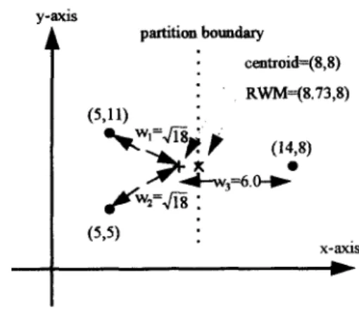
Example I (see Fig. 2). If the data are {(S,ll), (5,5), (14,8)}, then the centroid is (a, 9) = (8,B). Therefore, w1 = 11(5,11) - (S,S)] = dm = m w2 = II@, 5) - (8,S)ll = A-- 3* + 3* = diti, and w3 = ]](14,8) - (8, S)]] = 6. Since W=wt+w2+w3=2&8+6, the RWM is b’, Y’) with d = [a(S) + a(5) + 6(14)]/[2J18 + 61 = 8.73 (3) 2-D Data Fig. l(a) Fig. l(b)
Table 1. Total sum of squared error (TSSE) and CPU time (in s) for different algorithms RWM-cut Median-cut Mean-split Center-cut Variance-based TSSE/time TSSE/time TSSE/time TSSE/time TSSE/time 21047/0.0007 45333/0.0011 43756/0.0003 43756/0.0003 21678/0.0018
580 C.-Y Yang and J.-C. Lin y-axis t pa&ion boundary cenuoid=(8,8) - RWI+(8.73,8)
Euclidean distance.) After the computation, we found that Var(A) > Var(B); we therefore split class A. The RWM RR of class A is computed and the partition boundary is the line @ine 2 in Fig. 3(c)] passing thrzugh the RWM RA and perpendicular to the line OARS. Class A is therefore split into two finer subsets, namely, classes Aa and Ab. Since we already have three classes {B,Aa,Abj. and the expected number of classes is four, we have to split the data once more. After comparing Var(Aa), Var(Ab), and Var(B), we found that Var(B) is the largest; we therefore split B. The procedure is analogous to the one that we split A, and the resulting two smaller subsets are the Ba and Bb shown in Fig. 3(d). The final output of the system is the {Aa,Ab,Ba,Bb} shown in Fig. 3(e).
(5,ll) :
X-axIS *
Fig. 2. A 2-D example showing how to evaluate the RWM so that the given data can be split into two classes. The given data are {(5,11),(5,5),(14,8)}. Note that the partition boundary is through the RWM and perpendicular to the line connecting the centroid and the RWM. Also note that
each wi is a distance
y’= [J18(11) +J18(5) +6(8)]/[2J18+6] = 8. (4) If we want to partition this (2-D) data set into two classes, the partition boundary would be the (1-D) line passing through the RWM point (8.73,8) and perpendicular to the line connecting the centroid (8,8) and the RWM (8.73,8). From Fig. 2, we can see that {(5,11),(5,5)} is a class, while {(14,8)} is the other class.
The next example shows how we split a data set into more than two classes.
Example 2 (see Fig. 3). Let the data be the four- class data set shown in Fig. 3(a). First, we compute the centroid [represented by a “ + ” in Fig. 3(b)] and the RWM (represented by an “ x “) of the whole data set. Then the data set is split into classes A and B by the line [line 1 in Fig. 3(b)] passing through the RWM and perpendicular to the line connecting the centroid and the RWM. Now, we have to determine whether class A or class B should be split. Let OA and 0~ be the centroids of classes A and B, respectively. Simi- larly, let ]A] and ]B] be the number of points in classes A and B, respectively. The variances are defined as
Var(A) = c
II(Xi7
Yi) - o.4112/IAl (.%yrW--fand
“dB) =
C
IICxi, Yi) - oBl12/14,
h~r)eclarsB
respectively. (The norm symbol denotes the
Having seen how 2-D data can be partitioned using RWM, we give below the 3-D RWM-cut algorithm used to construct a color palette. Let
S={(ri, gi, &)ji= 1,2,...,/S]} be the given 3-D data set to be partitioned. The centroid (r:. jjj $) of S is evaluated by
is/ i-y& Ck i=,
The RWM (r’, g’, b’) of S is defined by extending the 2-D definition to 3-D case:
(8)
b’ = $ fJ biWi, Gl where W = 2 wi = fJ hi - F)’ + (gi - 2)’ + (bi - 6F. i=l i=l (11) Note that Wi is the distance from the centroid (P, g, 6) to the ith point (ri. gi, &). Once the RWM R=(r’, g’, P) and the centroid 0 = (F, g, 6) are known, the decision boundary proposed here to split:.. ..; .~ ; ,I ‘. .I
(4
Class Bb ” Class Aa B,, ‘;;‘,:,:.. :Fig. 3. A 2-D example showing how the RWM-cut algorithm splits a data set into four classes. The input is (a), and the final output is (e). Each “ +” represents a centroid, whereas each “ x ” represents an RWM
582 C.-Y. Yang and J.-C. Lin the given set S into two smaller subsets is then taken
to be the plane passing thrzugh the RWM R and perpendicular to the line OR The technique parti- tions a data set into two subsets, and we can repeat the technique K- 1 times to obtain K mutually disjoint subsets. The method proceeds in a hierarchi- cally divisive manner. The details of the method are described in the following algorithm.
Algorithm. The design of a color palette by the 3-D RWM-cut.
Input: a data set S = {(ri, gi, bi)li = 1,2,. . , ISI} and a predetermined value K.
Output: a K-color palette C = ((3, gj, h)I 1 <i < K}. Method:
Step 0: Initially, let cell cl be the entire data set S and go to Step 2.
Step 1: Choose the cell c/ with the largest variation for further partition.
Step 2: Compute the centroid 0 = (r, g, 5) of the cell cl.
Step 3: Compute the RWM R=(r’, g’, b’) of the cell cl.
Step 4: Partition cell cl into two smaller cells. The partition boundary is the plane passis through R and perpendicular to the line OR (When 0 = R, although this case seldom occurs, just take the partition boundary to be the plane passing through R and perpendicular to the coordinate axis with the largest variance.) Step 5: Repeat Steps l-4 until the number of cells reaches K.
Step 6: Collect the centroids of the K cells. These centroids form the K desired representative colors. Therefore, a K-color palette C has been produced.
Step 7. Stop.
3. EXPERIMENTAL RRSULTS
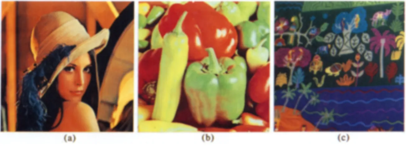
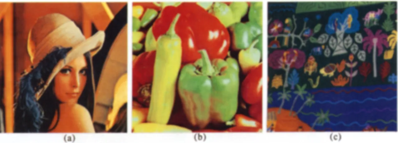
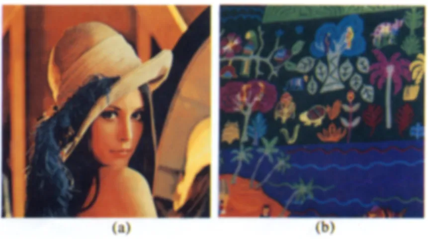
Three full-color 512 x 512 images, namely, Lena, Peppers, and Painting, are shown in Fig. 4. Each
RGB pixel of these three input images is represented by 24 bits, 8 bits per component. All tests were implemented on a Sun SPARC 10 workstation. Our simulations were performed with the following two aims: (i) to know the MSE and execution time when the RWM-cut algorithm is used alone, and (ii) to show that the RWM-cut algorithm can be used to generate a good initial palette for the LBG algorithm. In (ii), we also list the experimental results when the LBG algorithm is equipped with other kinds of initial palettes, such as the palettes generated by the median-cut, uniform quantization, and mean-split algorithms.
The RWM-cut algorithm was first applied to quantize the three input images to 256 colors. The 256-color quantized images generated by the RWM- cut algorithm are depicted in Fig. 5. The MSE and execution time produced by the RWM-cut algorithm, and by the LBG algorithm with a random initializa- tion, are shown in Table 2. Note that there is nothing to be initialized in the RWM-cut algorithm, while the LBG algorithm will need to choose the initial palette carefully. We then tried to improve the performance of the LBG algorithm by using a better initial palette. The four initial palettes used were the palettes generated by the RWM-cut, median-cut, uniform quantization, and mean-split algorithms, respect- ively. The results are given in Table 3. The LBG algorithm is stopped when no obvious improvement is made between two consecutive iterations. The threshold for stopping the LBG algorithm is the same for these four approaches. We can see that the RWM-cut is the best among these four approaches.
4. REAL-TIME APPLICATIONS
For real-time applications, many authors used a pre-processing to truncate the 24 bit input image to a 15 bit image, and then apply their color quantization methods to this partially quantized image. In the following, we will also use this pre-processing. The 24 bit image is reduced to a 15 bit image first, with 5 bits for each of the RGB components (that is to
say, we discard the three least significant bits for each 8 bit component). A (modified) 1-D RWM-cut algorithm is then hierarchically applied to the coordinate component with the largest variance. (Using 1-D RWM-cut is faster than using 3-D RWM-cut.)
Below we illustrate how to partition a 3-D data set into two subsets using a 1-D RWM-cut algorithm. First, inspect the variance in each of the three coordinate components {R,G,B}. Without the loss of generality, let H = {hi]i = 1,2, . . , Iq} be the 1-D component with the largest variance. The centroid z of H is then defined by
(14
Analogously, the RWM h’ of H is defined by
h’ = (g wih)/( f$ wi) (13)
with wi = ]hi - 61 for all i. The decision boundary used to split the 3-D data set into two subsets is then
taken to be the plane intersecting the component axis at h’, and perpendicular to the component axis. The procedure is repeated K - 1 times until the desired K subsets are obtained. The detail is omitted.
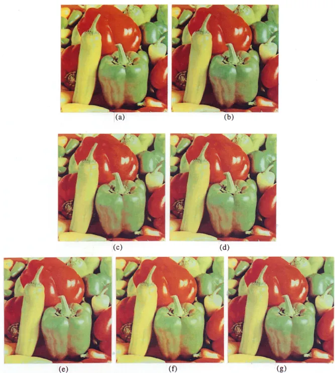
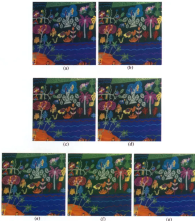
According to [9], the 5-6-4 bit-allocation [shown in Figs 6(b), 7(b), and 8(b)] was used as the 15 bit version for the center-cut algorithm. As for the remaining algorithms, the 5-5-5 bit-allocation [shown in Figs 6(a), 7(a), and 8(a)] was used. The 256-color Lena generated by different algorithms are shown in Fig. 6. Similarly, the 64-color Peppers and Painting produced by different algorithms are shown in Figs 7 and 8, respectively. Some wrong blue dirty spots appear on the hat and inside the mirror in Fig. 6(d) (the median-cut algorithm), while a long (but not too obvious) red scar appears on the right cheek of Lena in Fig. 6(g) (the variance-based algorithm). On the other hand, although the perceived quality of Fig. 6(f) (the center-cut algorithm) is better than those of Fig. 6(c) (the RWM-cut algorithm) and Fig. 6(e) (the mean-split algorithm), the color hue of the quantized image is somewhat too yellow in Fig. 6(f), as is compared with Fig. 4(a). (In fact, the color hue is still not quite right in Fig. 7(f) where the red peppers and the white reflection are too yellow [cf: Fig. 4(b)].) In the right part of Fig. 8(d) (the median-cut algorithm) and Fig. 8(e) (the mean-split algorithm), some orange-color spots appear on the two red plants,
Table 2. Performance of the RWM-cut algorithm and the LBG algorithm with random initialization
24 bit images No. of colors MSE/time (s) RWM-cut LBG algorithm MSE/time (s)
Lena 16 15.16/18.25 20.391359.32 32 11.08/21.83 18.10/708.10 64 8.81j25.75 11.70/1223.98 128 6.85/29.57 8.20/1948.64 Painting 16 15.75/18.78 19.39/368.69 32 12.12127.72 12.20/743.30 64 10.76/32.75 11.00/1192.84 128 9.28/39.90 10.79/1952.49
584 C.-Y. Yang and J.-C. Lin
Table 3. MSE and execution time (in s) for the LBG algorithm with initial palette gzoerated by ditkreat algotitbms 24 bit images Lena Painting No. of colors 16 32 64 16 32 64 RWMcut Me&au-cut MSEjtime
UnifQnn quauti~on
r&SE/time MS&kime Mean-spiit MSWtitne 13.10/156.81 13.181275.07 13.421747.15 13:20/272.49 9.83/400.15 9.861490.72 11.07/1769.66 9.91p3.55 1.74/878.56 7.80/1403.44 10.83j2916.78 7.7%/1052.77 13.35/64.18 13.36/64.68 17.64/606.99 13.37f129.16 10.29/126.39 10.49/189.98 12.591753.84 10.67/126.41 1.43t495.61 7.45/!#0.06 12.3212124.22 7.45i620.43Fig. 6. The 256color quantized images generated by using ditferent algorithms on the 15 bit versions of .&ma. (a) The (S-5-5) 15 bit version, (b) the (5-6-4) 15 bit version, (c) the RWM-cut, (d) median-cut, (e)
Cd)
Fig. 7. The 64color quantized images generated by using different algorithms on the 15 bit versions of
Peppers. (a) the (5-5-5) 15 bit version, (b) the (5-6-4) 15 bit version, (c) the RWM-cut, (d) median-cut, (e) mean-split, (f) center-cut, and (g) variance based algorithms.
while the purple color of the third wave in the sea sea, waves, etc. are all wrong). The MSE (distor- becomes wrong. (For the mean-split algorithm, the tion from the 24 bit images) and execution time third wave even becomes broken or thinner, and generated by different algorithms for different the color of the pink palm is changed.) In Fig. 8(g) numbers of representative colors are provided in (the variance-based algorithm), white dots become Table 4. It is observed that the MSE for the too obvious on the pink palm and the third RWM-cut algorithm is quite often the smallest (purple) wave. As for Fig. 8(f) (the center-cut among these five quantization algorithms, and the algorithm), many colors are wrong (the colors of execution time for the RWM-cut algorithm is the pink palm, pink tree, green land, orange island, similar to the one for the mean-split algorithm
C.-Y. Yang and J.-C. Lin
Fig. 8. The M-color quantized images generated by using different algorithms on the 1.5 bit versions of Painting. (a) The (S-S-5) 15 bit version, (b) the (5-6-4) 15 bit version, (c) the RWM-cut, (d) median-cut, (e)
mean-split, (f) center-cut, and (g) variance-based algorithms.
(but shorter than those for the remaining three It is well-known that the subjective quality of algorithms). We therefore think that the proposed the quantized images can be improved by applyiag a RWM-cut algorithm is a method with small digital halftoning (or spatial dithering) technique. quantixation error and competitive processing Existing spatial dithering techniques include err& speed. Alao note that a very simple method, the diffusion [14, 151, o&red dithering [16, 17, and dot so-called uniform quantization method, is not listed diffusion [18]. Since contouring effects can -be here because that method was observed to give considerably alleviated by error di%usion, we -used false contours in most of the experiments. it in our experiments to improve the quality of the
Table 4. MSE and execution time (in s) for different algorithms+ when the 15 bit version is used in each input image 15 bit images
Lena
Peppers Painting
No. of RWM-cut Median-cut Mean-split colors MSEjtime MSE/time MSE/time 32 16.39/1.32 20.55/1.48 17.05/1.32 64 15.00/1.43 17.68/1.61 15.58/1.43 128 13.8511.57 16.19/1.78 14.02/1.56 32 18.99/1.35 22.30/1.50 21.01/1.34 64 17.21/1.50 19.51/1.62 18.4711.46 128 15.2911.57 17.59j1.79 15.92/1.57 32 16.89/1.33 17.81/1.49 17.8411.33 64 15.21/1.45 17.4211.63 15.76/1&I 128 13.68/1.57 16.0611.82 135911.57 Center-cut* Variance-based MSE%/time MSEjtime 21.20/1.47 17.38/1.68 20.15j1.57 15.74/1.80 18.92/1.76 14.86/2.01 25.0711.48 20.85/1.70 21.4711.61 17.97jl.92 19.48/1.76 16.17/2.12 24.1311.48 18.74/l .69 23.7611.63 17.06/1.92 22.07/1.80 15.64/2.02 +The LBG was not used.
tAlthough a post-processing, which uses the “24 bit” pixel values of the original image to modify the color palette, can be used to improve the color hue for the center-cut algorithm; the total computation time will make the algorithm less competitive in real-time application. Therefore, there is no post-processing throughout the paper presented here.
%ome other control polices can be used to alleviate the high MSE, but false contours will then appear in the images, and the major advantage of using the center-cut will then disappear.
quantized images. The main steps of the dithering technique are listed below:
for i: = 1 to M do for j: = 1 to N do begin e: = P [i, f -P ‘[i, j]; P]i,j+l]:=P[i,j+l]+ex7/16; P[i+l,j-l]:=P[i+l,j-l]+ex3/16; P[i+l,j]:=P[i+l,j+ex5/16; P[i+l,j+l]:=P[i+l,j+l]+ex1/16; end for end for.
In the above, both M and N are 512; P, P’, and e are the 3-D color values of the input image, the quantized image, and the difference between these two images, respectively. The 32-color dithered images of Lena and Painting are shown in Fig. 9. As expected, with dithering technique, a 32-color quantization is also not bad.
5. SUMMARY
In this paper, we have proposed a new simple method that uses the radius weighted mean (RWM) to generate color palettes. Experiments show that the RWM-cut algorithm is feasible and visually accept- able. When used alone, the method is more reliable and much faster than the LBG method if random initialization is used in the LBG algorithm. The method can also be regarded as a good initial palette generator for the LBG method. This was confirmed by our experiments, which compared the MSE produced by the LBG algorithm when the initial palette was generated by the RWM-cut algorithm and by other well-known methods. Besides the proposed 3-D RWM-cut algorithm, we had also proposed a simplified I-D RWM-cut algorithm to quantize colors for real-time applications. The quantization error is small and the processing speed is competitive. In other words, a visually acceptable result can be obtained by the proposed RWM-cut algorithm in a reasonable amount of time.
(a)
(b)
Fig. 9. The 32-color dithered images generated by using the RWM-cut algorithm on the 15 bit version of (a) Lena and (b) Painting.
588 C.-Y. Yang and J.-C. Lin Acknowledgement-This work was supported by the Na-
tional Science Council, Republic of China, under grant NSC85-221%EOO9-111.
REFERENCES
1. S. J. Wan, P. Prusinkiewicz and S. K. M. Wong, Variance-based color image quantization for frame buffer display. Color Research and Application 15, 52-
58 (1990).
2. Y. Linde, A. Buzo and R. M. Gray, An algorithm for vector quantifier design. IEEE Transactions on
Communications 28, 84-95 (1980).
3. P. Heckbert, Color image quantization for frame buffer display. Computer Graphics 16, 297-307 (1982). 4. B. Kmz, Optimal color qua&&ion for color displays.
In Proceed-bgs of IEEE-Computer Vision and P&&n Recoanition Conference. 217-224 (1983).
5. X. Wi and I. H: Wit&, A fast k-&a& type clustering algorithm. Technique Report, Department of Computer Science, University of Calgary, Calgary, Canada (1985). 6. S. J. Wan, S. K. M. Wong and P. Prusinkiewicz, An algorithm for multi-dimensional data clustering. ACM
Transactions on Mathematical Software 14, 153-163 (1988).
7. M. T. Orchard and C. A. Bouman, Color quantization of images. IEEE Transactions on Signal Processing 32, 2677-2690 (1991).
8. X. Wu, Color quantization by dynamic programming and principai analysis. ACM Transactions on Graphics
11, 348-372 (1992). 9. 10. 11. 12. 13. 14. 15. 16. 17. 18.
G. Joy and Z. Xiang, Center-cut for color-image quantization. The Visual Comuuter 10. 62-66 f19931.
A. Mitiche, and J. K. Agga&l, Contour re&ra& by shape-specific point for shape matching Computer
Vision, Graphics and Image Processing 22, 396-408 (1983).
J. C. Lin, S. L. Chou and W. H. Tsai, Detection of rotationally symmetric shape orientations by foid- invariant shape-specific points. Pattern Recognition 25. 473-482 (1992).
J. C. Lin and W. H. Tsai, Feature-preserving clustering of 2D data for two-class problems using analytical formulas: an automatic and fast approach. IEEE Transactions on Pattern Analysis and Machine Intelligence 16, 554-560 (1994).
Y. T. Cb.ien, Interactive Pattern Recognition, Marcel Dekker, New York (1978).
R. W. Floyd and L. Steinberg,An adaptive algc&hm for spatial gray scale. Proceedings of SZD 17, 75-71
(1976).
J. F. Jarvis, C. N. Judicc and W. H. Ninke, A survey of techniques for the display of continuous tone pictures on bilevel displays. Computer Vision, Graphics and Image Processing 5, 13-40 (1976).
R. A. Ulichney, Digital Halftoning, MIT Press, Cam- bridge, MA (1987).
A. K. Jain, Fundamentals of Digital Image Processing,
Prentice-Hall, New Jersey (1988).
D. E. Knuth, Digital halftones by dot diffusion. ACM