Three-dimensional PAC video codec for wireless data transmission

(1)

IEEE TRANSACTIONS ON CIRCUITS AND SYSTEMS FOR VIDEO TECHNOLOGY, VOL. 10, NO. 8, DECEMBER 2000 1455

Three-Dimensional PAC Video Codec for Wireless

Data Transmission

Kuei-Ann Wen, An-Yi Chen, Yin-Jin Lan, Jun-Lin Lin, and Chia-Huang Lin

Abstract—A newly derived algorithm called three-dimensional polynomial approximation coding (3DPAC) is being utilized in the applications of wireless video transmission. After combining the spatial and temporal domain, the video data is organized in a cube form, which has the features of processing parallelism and great compression ratio. Such a very low bit-rate video codec is able to support the wireless data transmission with a bit rate lower than 9.6 kbits/s. The system architecture will be presented and an ex-perimental demonstration is also shown. For a video sequence of 176 144 frame size, PSNR up to 35 dB maybe obtained under 6.5 kbits/s transmission rate.

Index Terms—Combined source coding and channel modula-tion, entropy coding, multimedia communicamodula-tion, variable bit rate coding, videocoding.

I. INTRODUCTION

N

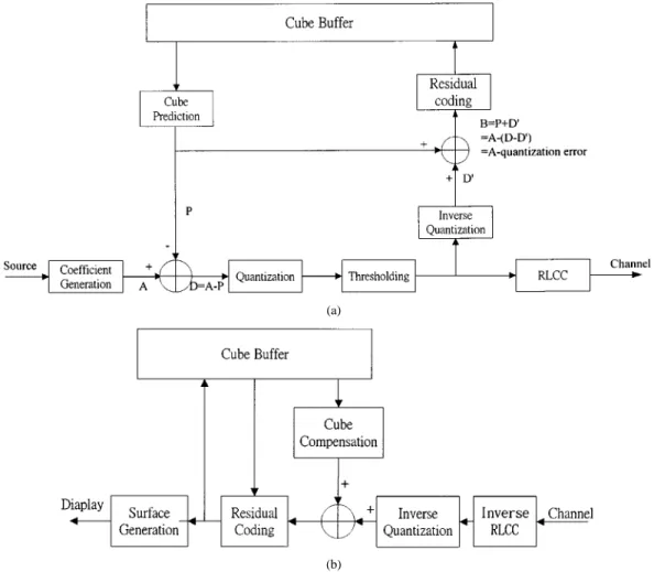
OWADAYS, multimedia communication has become one of those most actively developed topics in both academic and industry. Under the fast development of mobile communi-cation, home RF, and wireless LAN, most of the applications of multimedia and personal communication are going wireless. Limited spectral provided by various wireless systems can be from 11 Mbits/s down to 9.6 kbits/s. High compression ratio and low architectural complexity will be the key factors for video to be transmitted wirelessly. Being extended from the 2-D polyno-mial approximation coding in Lu’s [1] and other related works, the 3-D polynomial approximation coding video codec (3DPAC VCodec), which is a DPCM system, has been designed and de-veloped. For featuring a very high compression ratio and a very low structure complexity, the bit rate of this 3DPAC VCodec can be 9.6 kbits/s or even lower with the satisfactory subjective quality maintained, this system is highly feasible and applicable to wireless transmission.

The 3DPAC VCodec is illustrated in Fig. 1. The major blocks include “coefficient generation,” “cube prediction,” “thresholding,” and “residual coding.” The source (video data) first enter the block-coefficient generation to go through the polynomial approximation coding to generate the coefficients (its reverse process in the decoder part is called “surface

generation”), which approximately represent the information

of the data. In order to eliminate the redundancy owing to the

Manuscript received September 10, 1998; revised February 7, 2000. This paper was recommended by Guest Editor K. N. Ngan.

K.-A. Wen and C.-H. Lin are with the Institute of Electronics Engineering, National Chiao-Tung University, Hsin-Chu, Taiwan.

A.-Y. Chen and J.-L. Lin are with Philips Research East Asia—Taipei, Taipei, Taiwan.

Y.-J. Lan is with Hsinchu Science-Based Industrial Park, Taiwan, R.O.C. Publisher Item Identifier S 1051-8215(00)08586-4.

temporal and spatial similarity and continuity of the video data, a so-called block “cube prediction” is designed (its reverse process in the decoder part is called “cube compensation”). Since the known datum is employed as the arguments in the processing of cube prediction, a “cube buffer” is required to store the previous coefficients. As depicted in Fig. 1(a), the symbol stands for the original coefficients, for the predicted ones, is the difference between the original coef-ficients and the predicted coefcoef-ficients, and is the set of the coefficients to be preserved in the prediction buffer. In order to achieve even greater performance, there are two extra blocks, “thresholding” and “residual coding,” designed before “run

length cube coding” (RLCC). As to the “residual coding,” it is

a newly derived smoothing algorithm to deal with the blocky effect due to the processes of “quantization,” “thresholding,” and “inverse quantization.” More detailed descriptions of this 3DPAC VCodec will be provided in the later sections.

Beside, without transform-based computation, a transpose buffer is not required, and thus hardware complexity can be lowered.

II. 3DPAC VCODECALGORITHM

The procedures for both encoder and decoder can be depicted below.

Encoding process:

1) generate coefficients from the gray-level input of pixels; 2) derive the predicted coefficients from the previously

known cubes;

3) subtract the exact reference coefficients from the pre-dicted ones and then send the difference to quantization; 4) perform “thresholding” to obtain higher compression

ratio;

5) Recover the quantized datum and send them to residual coding to increase PSNR and for the better subjective quality of video;

6) send the data out of thresholding to tje RLCC block to reduce the redundancy of datum;

7) send the final data to entropy coding and then to channel coding.

Decoding process:

1) get data from channel decoding and proceed entropy de-coding;

2) execute inverse RLCC to get the quantized datum; 3) push the quantized datum through inverse quantization; 4) derive the predicted coefficients from the previously

(2)

(a)

(b) Fig. 1. 3DPAC VCodec. (a) Encoder. (b) Decoder

Fig. 2. Example of edges and corners. (a) Original. (b) First-order approximation. (c) Second-order approximation

5) add the predicted coefficients with the results of inverse quantization and then get the approximated coefficient that is close to the actual coefficients;

6) perform residual coding on the coefficients and then store them in the prediction buffer;

7) compute and send out the decoded pixels with proper syn-chronization to the display equipment.

A. Coefficient Generation

In view of the polynomial approximation techniques, a 3-D chart of – -luminance is used to demonstrate a 2-D image. In Fig. 2(a), which represents the original luminance of a certain frame, there are sharp edges and corners; while after being ap-proximated with first-order and second-order polynomial

equa-tions, i.e., and

, as illustrated, it can be seen that with higher order approximation, the mathematical models will be more pre-cise at edge and corner while less difference at smooth surface.

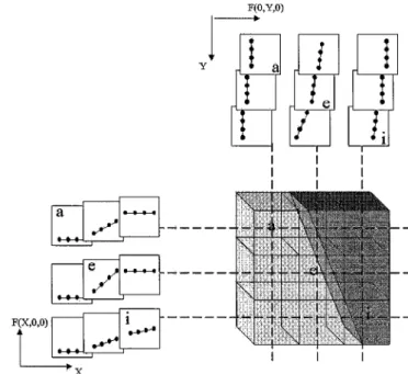
For video sequence, both spatial and time domains are mapped into the three coordinate axes, as shown in Figs. 3 and 4. The -axis points go from left to the right direction and the -axis points are from upper to the lower direction to construct the 2-D spatial domain, and the axis points to the time direction, just like the scan order of the video sequence of frames. In our model, though the center of the cube is located at the origin (0, 0, 0) and each pixel has the unit distance from neighboring pixels, somehow they are not with the normal index system to describe their position. For example, in

block size, the first pixel of the first frame has a coordinate of ( ), and the last pixel of the last frame that of

(1.5, 1.5, 1.5). That is, .

The reason for such a definition is to take the convenience and simplicity when it comes to computation, that is, we just perform shift-and-add instead of multiplication of the value of

, , coordinate.

If the gray level of the pixel ( ) of a video sequence is to be represented perfectly with a 3-D polynomial function, it would require an infinite order function. In other words, the better the approximation is, the more terms are needed for the function. This model description will be set out with a second-order polynomial approximation:

(3)

WEN et al.: 3-D PAC VIDEO CODEC FOR WIRELESS DATA TRANSMISSION 1457

Fig. 3. Graphical illustration of the pixel locations in a cube.

Fig. 4. Graphical illustration of the pixel coordinate in a cube.

where is a constant and the mean square error

(MSE) is

MSE (2)

with equally transmitted probability

MSE (3)

where is the number of pixels in a block (64 in a

block or 512 in an block). The summation is taken over all the indexes of , , and as assigned previously, then the coefficients can be obtained in consideration of minimum MSE for

(4) because of the property of symmetry, the summation of those

odd symmetric terms such as and are zero. This

simplifies (3) to be

(5) for the minimum MSE with respect to , the left side of (4) should be zero, and then

(6)

Similarly, C1 will be processed and the result would be (7) and

(8) Similarly, will be processed and the result would be

(9)

and the odd symmetry terms such as and are

also zero and the equation is simplified to

(10) For , there are more terms eliminated

(11) and

(12) To sum up, the group of equations with the coefficients men-tioned above are collected here

(13)

With (13), the simultaneous equations can be derived in ma-trix form and the mama-trix element (cube) scan order will be from left to right ( -axis), then from up to down ( -axis), and then from front to rear ( -axis), as shown in (14), at the bottom of the next page. Therefore, with the example of cube and second-order polynomial approximation, the matrix named contains the approximated luminance information that would be generated with (13) and (14) (see (15), shown at the bottom of the page). The coefficient matrix is in the form of

(16) Therefore, the mapping matrix is shown in (17), at the bottom of the page. The mapping relationship would be

(4)

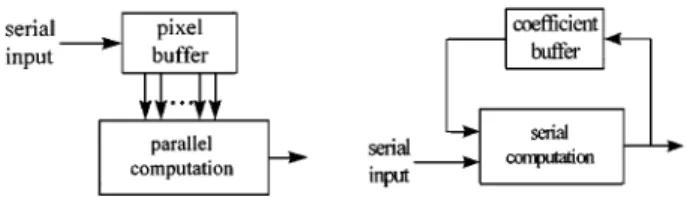
Fig. 5. Computation modes for 3DPAC VCodec. (a) Parallel mode. (b) Serial mode (PSO).

Fig. 6. Transition of the active cube.

Since is not a square matrix, it could be easier to deal with by the transpose and inverse calculation, and coefficient

matrix will be generated after several stages, which are shown below

(19) (20) where .. . (21) (22) (14) (15) .. . (17)

(5)

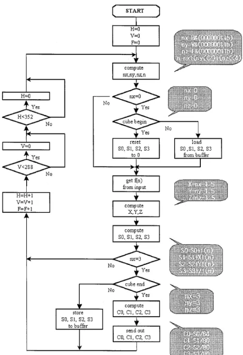
Fig. 7. Flowchart of the coefficient generation block

and

After all the computations, those elements of , that is, the coefficients of the approximated polynomial coding, will be quantized after a subtractive process and then be encoded by RLCC for video signal transmission. The decoder at the receiver would be another matrix operation processor to recover the function to work with the video-sequence playback.

1) Computational Simplification: Computation

simplifica-tion is highly and strictly demanded for wireless applicasimplifica-tions. To represent the gray level of every pixel in a cube in an efficient way, th-order polynomial approximation has been treated and, experimentally, it has already been proved that the 1st order approximation may get the best tradeoff of error per-formance and simplicity [1, Appendix]; that is

(23) To represent the gray levels of the 64 pixels in the cube, we just need to give the four polynomial coefficients , , , and , instead of the data of 64 pixels. Utilizing the cube size and first-order polynomial approximation, within this

(6)

cube-based block, the four coefficients will be generated with the matrix computation, as previously obtained in equation (19) (24) where

coefficient matrix of four elements; pixel matrix of 64 elements; constant computation matrix.

With computation simplification, the specified index of can be pre-computed and the matrix computation of can be implemented with simple calculations as

(25)

where and is the

pixel value in the corresponding position.

Further, the multiplication of 0.5 and division of 64 can be implemented by merely shifting the bit of coefficient, and the multiplication of 1.5 can be implemented by addition with mul-tiplication of 0.5. Thus, in this system, only the division of 80 requires a more complicated mathematical process.

2) Buffer Cost Reduction: Unlike the transform-based

com-putation, the previous summations do not make it necessary that all the pixels to have arrived to process. The traditional parallel mode of computation or transpose memory as demanded for the DCT-based system may not be required anymore. The PSO de-veloped and applied in the experiment of this work release the need for a large buffer. The buffer size reduction ratio is ob-tained as shown in (25a), at the bottom of the page.

With parallel computation, computation of coefficients will not be made until 64 pixels of a cube are fully collected, and it would cost the capacity of 64 pixels, or 512 bits if 8 bits for a pixel gray-level value for a single cube. However, in the PSO mode, computation starts as a pixel comes in and the uncom-pleted coefficients are then stored to the buffer for accumula-tion/summation. Hence, the computation of each cube will cost

Fig. 8. Gray-level transition along three virtual axes.

(a)

(b)

Fig. 9. Example of an edge within a frame. (a) Four cubes on the edge. (b) Coefficients of the four cubes.

the capacity of four coefficients. During the process, the max-imum of occurs when all the pixels are of gray level 255, that

is, , each coefficient maximally

needs 14 bits, and the buffer size required is

Buffer size (bits) (26)

where

(7)

Fig. 10. The available prediction directions.

Therefore, for a screen, the size of the coefficient buffer is about 354.8 kbits and that for a screen is 88.7 kbits, and the buffer-size reduction ratio is

(27)

3) Flowchart of Coefficient Generation: However, the

pixels come in the scan order, which is somewhat different from the order of the cubes. Fig. 6 illustrates the transition of the active cubes.

The flowchart of coefficient generation is shown in the Fig. 7. According to this flowchart, the following variables are com-puted in turn.

1) , , : the position of the active pixel corresponding to the whole video sequence in each direction.

2) , , : the position of the active pixel corre-sponding to the active cube in each direction.

3) : the number of pixels that the active cube has received. 4) , , : the coordinates of the active pixel in the active

cube.

5) : the temporary recursive summation for each coef-ficient.

6) : the 3DPAC coefficients which is generated after 64 pixels have arrived and the recursive summation is com-pleted.

B. Cube Prediction

After the transformation of source data to coefficients in coef-ficient generation, many of the cubes are highly correlated with each other for the continuity owing to the existence of an edge crossing the adjacent cubes. The relationship between neigh-boring cubes has been studied and observed in order to derive algorithms and schemes to increase the compression ratio.

Fig. 11. VariousW versus V .

1) Gray-Level Transition: To explain the algorithm of cube

prediction, it will be started with the gray-level transition de-scribed in Fig. 8. For each of the cube, a 2-D coordinate is formed with horizontal axis indicate the four discrete pixels ( ) in a cube and with vertical axis indicates the gray level, i.e.

(28) Similarly, we can get another set of 2-D coordinates with ver-tical denotes the four pixels ( ) and with horizontal axis indicates the corresponding gray-value -axis at (0, 1.5, 0), (0, 0.5, 0), (0, 0.5, 0), (0, 1.5, 0) with

(29) and at (0, 0, 1.5), (0, 0, 0.5), (0, 0, 0.5), (0, 0, 1.5) when the

direction is taken into account

(30) The values obtained by these three equations will be the basis to analyze gray-level transition between adjacent

(8)

(a) Fig. 12. (a) Flowchart of the direction decision.

cubes according to what direction is considered. Additionally, the coefficient left, other than , defined as the “dominant co-efficient,” is for the , for the , and for the direc-tion. It is because, as illustrated in Fig. 9(b), cubes with a higher gray level imply a larger value of and thus will dominate the gray-level change in the direction.

For example, in Fig. 9, the edge is more vertical and less horizontal, and therefore the ’s of the left two cubes are smaller and closer to zero because of less change. Abstractly, ’s are much larger. The dominant coefficient scales the degree of change of a single cube in a specified direction, simply and clearly.

1) It is almost piecewisely linear, and the contrast of edge is visualized with the slope

2) At the virtual origin point in each cube, where , , and are also zero, the recovered pixel is , which also stands for the average value of 64 pixels in the cube.

3) The transition view values of direction seem to be more similar and more highly correlated. and are more similar. Such a feature is called “reflectivity,” for the hor-izontally spatial continuity of the image is reflected at the tendency of lateral-view values at the relative direction. 4) Both in and directions, the boundaries of

neigh-boring cubes on the common face will be very close to each other. Such a feature is called “connectivity.”

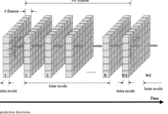
2) Cube-Prediction Algorithm: Fig. 10 provides the

predic-tion model with intra and inter cubes being defined. Coefficients of intra-mode cubes can be predicted for intra-mode cubes with the following prediction process.

a) Direction Decision: Two parameters, and , are defined for a direction decision

(31) (32)

(9)

(b) Fig. 12. (Continued.) (b) Flowchart of the cube prediction.

In the two equations above, the constant 1 is added to both di-vider and dividend in order to prevent the didi-vider from zero. The larger is, the more possibly the edge is extending in the direction. Conversely, large means the edge extends in the

direction.

The direction decision is made by comparing the conditions of and in both the previous and cubes as follows:

a) the first “wall” of cubes within a period, say cubes or frames, will be labeled as inter mode cubes, where no prediction is performed;

b) for the interframes, the prediction direction is forced to be in the direction;

c) for the intraframes, if one or both of and

is larger than the lower limit ( ), choose the direction corresponding to the larger one;

d) for the intraframes, if both are smaller than the lower limit

( ), compare and , and

choose the direction corresponding to the smaller one.

b) Prediction: After the direction is decided, the

predic-tion will be performed. The predicpredic-tion equapredic-tions are described in the following paragraphs.

The variance is defined as the absolute sum of two domi-nant coefficients at the direction previously chosen

(33) The larger is, the less connectivity there would be between two neighboring cubes. Thus,

for the direction:

(10)

for the direction

(35) and for the direction

(36) where is a weighting function of obtained with ex-perimental calculation and statistic with many benchmark se-quences, such as “Miss America” and “Miss Claire” [1]. Statis-tically, approximates to a constant 1.8, and others ap-proximate to linear functions of .

3) Flowcharts of Cube-Prediction Algorithm: Procedures

for cube prediction are illustration by flowchart in Fig. 12.

C. Thresholding

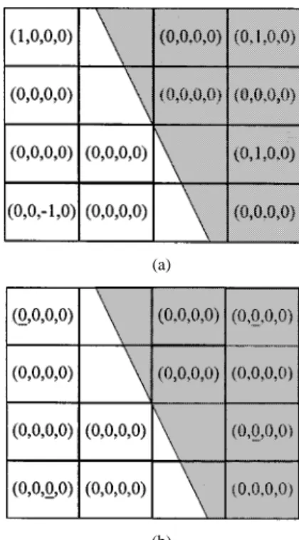
Since coefficient prediction shrinks the data size and hugely centralizes the data at the value of zero and after quantization, coefficients of most cubes become small value. The major func-tion of thresholding coding is to ignore such small values, as shown in Fig. 13. A cube with the quantization result of (0, 0, 0, 0) is called a zero cube here, while thresholding coding is to in-crease the number of zero cubes for the further channel coding.

After thresholding processing, the four quantized coefficients of a zero cube can be replaced with merely leading bits in vari-able-length cube coding. More zero cubes are produced and clustered, more redundant datum can be eliminated by VLCC, and the compression ratio can be even greatly increased.

A parameter is defined as

for intraframes

for

(37)

When gets small enough, it can be replaced by zero. There-fore, a threshold for has to be found and set with further calculation and statistics. Table I gives the simulation result, while Fig. 14 shows the performance of thresholding at different threshold values, and “missa ” means the Miss America se-quence processed with quantization step size . Thus, it is found that the reasonable threshold is set to one for further simulation and analysis.

The flowchart of thresholding process is given in Fig. 15 with the example thresholding value of 1.

D. Residual Coding

Even if the thresholding process does lose some unimportant information, such an error, in fact, does not harm the

subjec-(a)

(b)

Fig. 13. Zero cubes for thresholding. (a) Original quantization result. (b) After thresholding is applied.

TABLE I

PSNR DROP BYTHRESHOLDING

(a)

(b)

Fig. 14. The improvement of compression ratio by thresholding.

tive quality so much in the temporal domain because the human visual system is not as sensitive to thresholding noise in the tem-poral domain as the frame rate is reasonably high. However, in the spatial domain, the artifacts could corrupt the subjective quality at a certain degree. Hence, residual coding is derived and applied to smooth the blocky artifacts only in the spatial domain (see Fig. 16).

(11)

Fig. 15. Flowchart of thresholding.

Fig. 16. Illustration of spatial continuity and gray-level transition.

(a)

(b)

Fig. 17. Illustration of residual coding. (a) Virtual points (VPs). (b) Adjustment of VPs inX-axis.

Fig. 17 is an illustration of residual coding. At the two sides of the common face of two cubes, the gray-level transition graph may not be continuous or connected at all. That means that the image is not smooth at the adjacent border of these two cubes, and blocky artifacts exist. If the difference of the two ends of

(a)

(b) Fig. 18. Order of residual coding.

(12)

each cube’s gray-level transition can be approached and con-catenated, the visual performance is improved.

The main idea of residual coding is that, in Fig. 17(a), those virtual points on the faces of a cube will have to be moved closer in gray-level transition with the neighboring cube in spatial do-main, that is, and directions. First the gray level of the two

virtual points of a cube is:

(38) and the parameter diff is defined as

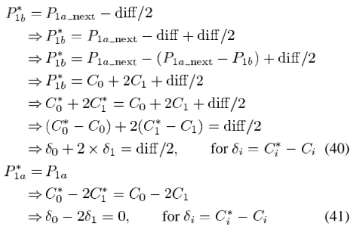
(39) is the VP at the position of P1a of the neighboring cube in the direction. Therefore, in order to shorten the difference of the two edges, as shown in Fig. 17(b), the adjustment is ap-plied to the two virtual points on the common face is diff , with the positive edge raised while the negative edge remained. Since is the coefficients after adjustment, the computation in the

X-axis is derived as follows:

for (40)

for (41)

With the results of (40) and (41), it is obtained that

and . However, the case in direction is

similar. Therefore, as both and directions are considered, the adjustment should be

(42) If diff happens to be large enough, it either indicates that an error exists, or an edge is actually nearby. In order to avoid per-forming this procedure to where there has to be a great gray-value difference, the offset adjustments will be performed only when the absolute value of diff is equal to or less than a certain threshold L, named “residual threshold”

(43) With the simulation results and analysis, the proper residual threshold is found to be 24.

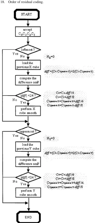
Fig. 18 shows the order of residual coding. The previously utilized cubes are stored in the buffer, which is also used in

(a)

(b)

Fig. 20. PSNR versus bit-rate curve. Dashed lines: residual coding effects. From top line down, the marks symbolize the thresholding of thresholdS at 0, 1, and 2, respectively, for (a) “Miss America” and (b) “Claire.”

TABLE II

THETRANSMISSIONRATE(KBITS/S)

cube prediction; therefore, no other buffer will be required in the system. When cube 354 comes, residual coding is performed on its upper ( direction) and left faces ( direction). In Fig. 18(b), when cube 355 comes, the right faces of cube 354 are also smoothed. Therefore, residual coding of a cube works in dif-ferent time. Fig. 19 shows the flowchart.

III. SIMULATION ANDANALYSIS

In the experimental work here for this system, the simulations are focused on the quantization, thresholding, residual coding

(13)

(a) (b) (c) (d)

(e) (f)

Fig. 21. Sample images: (a) Claire with quantization step 7 andS = 0: (b) Claire with quantization step 9 and S = 0: (c) Claire with quantization step 7 and S = 1: (d) Claire with quantization step 9 and S = 1. (e) Claire with quantization step 7 and S = 2: (f) Claire with quantization step 9 and S = 2.

(14)

TABLE III EVALUATION OF THEMODELS

individually, and the performance of a combination. In most of the simulation processes, we frequently employ the following two estimation functions:

(44)

(45)

In case the subjective observation for the system performance is necessary, the selected frames from the original coefficients and the decoded coefficients will be displayed.

The final simulation result is drawn in Fig. 20. Both thresh-olding and residual coding were applied. Dots marked in one line are applied with thresholding of threshold ( ) 0, 1, and 2, while quantization steps are equal to 7 and 9, respectively.

Thresholding makes the tradeoff between the compression ratio and video quality. It is found in Fig. 20 that the PSNR drops faster than the bit rate when the threshold increases from 0 to 2. Unless very low bit rate is demanded for a very narrow bandwidth, the thresholding at 2 is not recommended.

Residual coding not only has the ability of smoothing, but also improves the compression ratio. However, its performance is highly related to the nature of the video sequence. Its greatest contribution is the improvement of subjective quality. The sam-ples of Claire video clips may provide some demonstration.

Finally, the required transmission rate of various configura-tion is listed in Table II, in which “missa ” means the Miss America images of quantization step , and thresholding ( ) at . The configuration for a specified application should be chosen according to the provided channel bandwidth.

In Fig. 21, some example images processed with width-4 cube and first-order approximation are shown.The simulation time is 0.1 s/frame for encoding ( pixels per frame), and 0.05 for decoding, with a Pentium 233-MHz CPU and 32 MB RAM. So this scheme achieves real-time decoding for a 20 frames/s sequence.

Fig. 22. Frame 1 of video sequence “Claire” generated from various width and order.

IV. CONCLUSION

3DPAC has been derived to obtain a high compression ratio with simple circuitry for wireless video transmission. To achieve

(15)

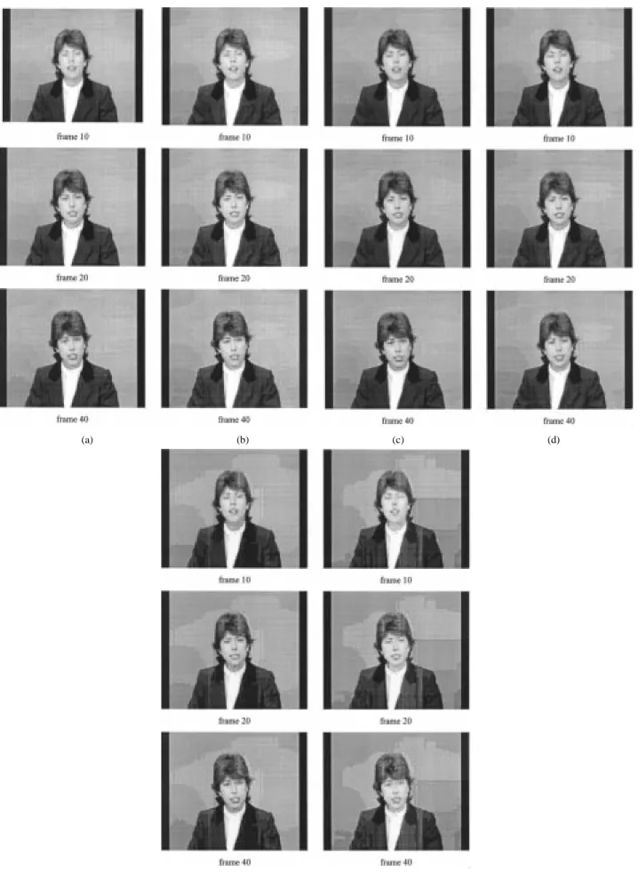
Fig. 23. Comparison with Frames 1, 3, 5, and 7 (50% of the original size, extracted from the video sequence “Claire”).

the high compression ratio, the DPCM structure combined with the characteristics of 3DPAC has been derived, and also the lossy thresholding process. It offers beneficial tradeoff between the compression ratio and the quality when the threshold is 1.

To increase the PSNR, the function block residual coding is proposed. Residual coding improves the video quality by the way somewhat like the titter-totter. It raises or lowers the edges of cubes so as to approach the neighboring edges. Besides, since the coefficients are modified, the cube prediction will performs better and the compression ratio is also improved.

Low circuit cost, little storage buffer, and fast speed are predictable because almost every function block is designed making computation only on coefficients. Besides, thresholding and residual coding require only addition and comparison, which takes little implementation area.

APPENDIX

The reason why the cube and first-order polyno-mial approximation are chosen for 3DPAC VCodec has been described in [9], and is briefly illustrated below.

In Table III, there are six types of models with two different widths and three orders. The cube-to-coefficient data ratio (CCDR), PSNR, and computation complexity (in the view of estimated multiplication) are of our concern. The simulation statistics of PSNR and CCDR are also included.

Where is defined to be judgement parameter which is a weighting function of CCDR, PSNR, and computation com-plexity, i.e.

(A.1) It is shown mathematically that the models of width-4 and order-1 and of width-8 and order-1 have much higher -values than the others, yet the comparisons of each other’s factors have clearly declared the performance of the models in several aspects of tradeoff consideration.

Furthermore, we have also made comparison of subjective performance on two of the models. Width-4-order–1 and width-8-order–1 both have outstanding -values and fairly good compression ratio; somehow we have to show the tradeoff with the visual quality. Several series of video sequence and frames are shown in Figs. 22 and 23.

REFERENCES

[1] C. Y. Lu, A. Y. Chen, and K. A. Wen, “Polynomial approximation coding for progressive image transmission,” J. Vis. Commun. Image Repres., vol. 8, no. 3, pp. 317–324, June 1997.

[2] M. Kocher and R. Leonardi, “Adaptive region growing technique using polynomial functions for image approximation,” Signal Process., vol. 11, pp. 47–60, 1986.

[3] E. Karabassis and E. Spetsakis, “An analysis of image interpolation, dif-ferentiation, and reduction using local polynomial fits,” Graph. Models Image Process., vol. 57, no. 3, pp. 183–196, May 1995.

[4] M. Eden, M. Unser, and R. Leonardi, “Polynomial representation of pic-tures,” Signal Process., vol. 10, pp. 385–393, 1986.

[5] L.-W. Chan, “The interpolation property of fuzzy polynomial approxi-mation,” in Proc. Int. Symp. Speech, Image Processing and Neural Net-works, Hong Kong, Apr. 1994, pp. 449–452.

[6] L. Corte-Real and A. P. Alves, “Vector quantization of image sequences using variable size and variable shape blocks,” Electron. Lett., vol. 26, pp. 1483–1484, 1994.

[7] M. Chan, Y. Yu, and A. Constantinides, “Variable size block matching motion compensation with applications to video coding,” Proc. Inst. Elect. Eng., pt. I, vol. 137, pp. 205–212, 1990.

[8] H.-M. Hang and B. Haskell, “Interpolative vector quantization of color images,” IEEE Trans. Pattern. Anal. Machine Intell., vol. PAMI-2, pp. 165–168, 1980.

[9] P. Cherriman, “Packet video communications,” Ph.D. dissertation, Dept. of Electron., Univ. of Southampton, Southampton, U.K., 1996. [10] L. Hanzo, “Bandwidth-efficient wireless multimedia communications,”

Proc. IEEE, vol. 86, July 1998.

Kuei-Ann Wen was born in Keelung, Taiwan, R.O.C., in 1961. She received the B.E.E., M.E.E., and Ph.D. degrees from the Department of Electrical and Computer Engineering, National Cheng-Kung University, Taiwan, R.O.C., in 1983, 1985 and 1988, respectively.

She is currently a Professor in the Department of Electrical Engineering, National Chiao-Tung University, Taiwan, R.O.C., and is also involved in several research projects from Wireless Communi-cation Consortium (http://wireless.eic.nctu.edu.tw) and Academic Center of Excellence (http://www.eic.nctu.edu.tw/ace/), under the supervision of the Department of Higher Education, Council of Academic Reviewal and Evaluation of R.O.C. Her research interests are in the areas of wireless communication system, RF circuit design, and video signal processing and transmission.

(16)

An-Yi Chen was born in Tainan, Taiwan, R.O.C., in 1971. He received the B.S. degree from the De-partment of Electrical Communication Engineering, National Chiao-Tung University, Taiwan, R.O.C., in 1993, the M.S. degree from the Department of Electrical and Computer Engineering, State University of New York at Buffalo, in 1995, and the Ph.D. degree from the Institute of Electronics, National Chiao-Tung University, in 2000.

He is currently a Research Engineer of the Infor-mation Appliance System Group, Philips Research East Asia–Taipei, Taipei, Taiwan. His research interests are in wireless video transmission, video signal processing, and circuit implementation.

Yin-Jan Lan was born in Tao-Yung, Taiwan, R.O.C., in 1973. He received the B.S. degree from the Department of Electrical Engineering, National Tsing-Hua University, in 1995, and the M.S. degree from the Institute of Electronics, Na-tional Chiao-Tung University, Taiwan, R.O.C., in 1997.

He is currently an Engineer in Hsinchu Science-Based Industrial Park, Taiwan, R.O.C.

Jun-Lin Lin was born in Hsinchu, Taiwan, R.O.C., in 1974. He received the B.S. degree from the Department of Electronics Engineering and the M.S. degree from the Institute of Electronics, both at National Chiao-Tung University, Taiwan, R.O.C., in 1997 and 1999, respectively.

He is currently a Research Engineer in the Infor-mation Appliance System Group, Philips Research East Asia–Taipei, Taipei, Taiwan. His research inter-ests are video compression and SoC design.

Chia-Huang Lin was born in Taipei, Taiwan, R.O.C., in 1976. He received the B.S. degree rom the Department of Electronics Engineering and the M.S. degree from the Institute of Electronics, both at National Chiao-Tung University, Taiwan, R.O.C., in 1998 and 2000, respectively.

Currently he is serving his obligatory military service. He will then join Spring Soft in Hsinchu Science-Based Industrial Park, Taiwan, R.O.C.