交通參數估測系統之攝影機參數校正與影像追蹤

全文

(1)國立交通大學電機與控制工程學系博士論文交通參數估測系統之攝影機參數校正與影像追蹤 Camera Calibration and Image Tracking for Traffic Parameter Estimation. 研究生：戴任詔指導教授：宋開泰博士. 中華民國九十五年七月.

(2) 交通參數估測系統之攝影機參數校正與影像追蹤 Camera Calibration and Image Tracking for Traffic Parameter Estimation 研究生：戴任詔. Student: Jen-Chao Tai. 指導教授：宋開泰博士. Advisor: Dr. Kai-Tai Song. 國立交通大學電機與控制工程學系博士論文 A Dissertation Submitted to Department of Electrical and Control Engineering College of Electrical and Computer Engineering National Chiao Tung University in Partial Fulfillment of the Requirements for the Degree of Doctor of Philosophy in Electrical and Control Engineering July 2006 Hsinchu, Taiwan, Republic of China. 中華民國九十五年七月 ii.

(3) 交通參數估測系統之攝影機參數校正與影像追蹤學生:戴任詔. 指導教授:宋開泰博士. 國立交通大學電機與控制工程學系. 摘要本論文主要探討運用於交通參數估測系統之先進影像處理技術，包括動態攝影機參數校正、背景影像建立、影子移除、車輛偵測追蹤與交通參數量測。進行交通參數估時，首先必須準確地校正攝影機參數，方能利用二維影像畫面來精確地求出物體於空間之三維物體位置，本論文設計一套可自動校正 Pan-Tilt-Zoom 攝影機參數之方法，發展出利用一組平行的車道標線與其在影像畫面中之幾何位置，產生焦距方程式來求焦距，再計算出其他攝影機參數值。在車輛偵測與追蹤前處理階段，一般利用背景影像移除方法將移動中車輛由影像畫面中分離出來，本論文提出基於群組直方圖 (Group-Based Histogram)方法，可快速建立良好之背景影像，此方法對於感測雜訊與慢速移動車輛具強健性。進行交通監測影像分析時，車輛的影子會造成車輛影像嚴重變形，甚至與其他車輛影像產生重疊，嚴重影響車輛偵測與追蹤的準確性。本論文利用影子色彩特性與統計方法，提出一個色彩空間比值模型，此模型可迅速偵測影像中之影子像素，配合兩種幾何分析方法再提昇影子偵測的準確性。以這個比值模型所設計的動態車輛偵測方法比現有方法更有效率。交通參數估測時，必須對多車道中大小不一之車輛進行追蹤，本論. iii.

(4) 文發展一套自動輪廓初始化方法，利用特殊設計之偵測窗來偵測進入影像畫面中多車道內任意位置且大小不同之車輛，並依據車輛大小與位置所產生車輛之初始追蹤輪廓，再利用卡曼濾波器進行追蹤，分析追蹤結果可得到車流與車速之交通參數。另外，針對 T 字路口轉彎率量測，本論文設計一套可即時判定車輛移動方向的光流偵測技術，並結合偵測窗來量測路口之車輛轉彎率。本論文所發展之方法理論，均已利用實際道路交通影像進行驗證，量測所得之交通參數，如平均車速、車流量、車流密度與轉彎率，誤差值在 5％內，顯示本論文所提出的方法確實能正確且快速完成交通參數估測。. iv.

(5) Camera Calibration and Image Tracking for Traffic Parameter Estimation Student: Jen-Chao Tai. Advisor: Dr. Kai-Tai Song. Department of Electrical and Control Engineering National Chiao Tung University. ABSTRACT The objective of this thesis is to study advanced image processing methodologies for estimating traffic parameters with functional accuracy. The developed methodologies consist of camera calibration, single Gaussian background modeling and foreground segmentation, shadow suppression, vehicle detection and tracking, and optical-flow-based turn ratio measurement. The accuracy of estimating vehicle speed depends not only on image tracking but also on the accuracy of camera calibration. A novel algorithm has been proposed for automatic calibration of a pan-tilt-zoom camera overlooking a traffic scene. A focal length equation has been derived for camera calibration based on parallel lane markings. Subsequently, the pan and tilt angles of the camera can be obtained using the estimated focal length. To locate the parallel lane markings, we develop an image processing procedure. In the preprocessing step of vehicle detection and tracking algorithm, foreground segmentation can be accomplished by using background removal. The quality of background generation affects the performance of foreground segmentation. Thus, a group-based histogram algorithm has been designed and implemented for the estimation of a single Gaussian model of a v.

(6) background pixel in real-time. The method is effective and efficient for building the Gaussian background model from traffic image sequences. It is robust against sensing noise and slow-moving objects. However, shadows of moving objects often cause serious errors in image analysis due to the misclassification of shadows as moving objects. A shadow-region-based statistical nonparametric method has been developed to construct a RGB ratio model for shadow detection of all pixels in an image frame. This method of shadow model generation is more effective than existing methods. Additionally, two types of spatial analysis have been employed to enhance the shadow suppression performance. An automatic contour initialization procedure has been developed for image tracking of multiple vehicles based on an active contour and image measurement approach. The method has the capability to detect moving vehicles of various sizes and generate their initial contours for image tracking in a multi-lane road. The proposed method is not constrained by lane boundaries. The automatic contour initialization and tracking scheme has been tested for traffic monitoring. Additionally, this paper proposes a method for automatically estimating the vehicle turn ratio at an intersection by using techniques of detection window and optical flow measurement. Practical experimental studies using actual video clips are carried out to evaluate the performance of the proposed method. Experimental results show that the proposed scheme is very successful in estimating traffic conditions such as traffic flow rate, vehicle speeds, traffic density, and turn ratio.. vi.

(7) 誌謝衷心感謝我的指導教授宋開泰博士，多年來，在專業上或處理事情上，真摯誠意且不厭其煩的給我指導及修正，使我受益良多，順利完成博士學業。感謝論文口試委員— 交通大學莊仁輝教授、中央研究院廖弘源教授、暨南國際大學王文俊院長、清華大學彭明輝教授與交通大學林進燈院長，給我的建議與指引，強化本篇論文的嚴整性與可讀性。感謝明新科技大學的支持，歷屆校長、各級長官、機械系主任、同事們的鼓勵與行政支援，讓我能盡全力進行博士班研究課業。感謝 ISCI 實驗室的學弟們多年來提供的協助，尤其是參與本論文初期研究的學弟，如舜璋、清波、辰竹，也感謝博士班學弟奇謚與孟儒對本論文的建議與討論，另外特別感謝十項全能的嘉豪，在軟體程式應用發展上各項協助。感謝教育部，由『下世代人性化智慧型運輸系統』卓越計畫提供的硬體設備與經費，讓許多實驗得以順利完成，並感謝林進燈院長的資訊媒體實驗室鶴璋學長出借 PTZ 攝影機，讓我順利完成動態攝影機參數校正實驗。也感謝謝明新科大專題學生，特別是建榮與文淇，在炎熱夏日中，進行道路交通影像拍攝，以供實驗進行。感謝父母與岳母的鼓勵與栽培，在父母重病其間，哥哥與姊姊的扶持提攜，公園教會兄姐的代禱，讓我能夠成長，完成學業。感謝內人美生體諒我就讀研究所博士班，課業繁重，協助我照料家庭，免除後顧之憂，並將全家一切需要放在禱告中，向全能的上帝祈求賜福，使我能潛心向學，最值得我感謝。也謝謝體貼人意的女兒涵妮與涵芸的加油與鼓勵，給予我無比的勇氣，但在你們成長的歲月，為人父的我，因為課業壓力沒有好好陪伴成長。希望在未來人生旅途上，全家都能在. 神保守下，和睦相愛。. 最後，感謝全能的上帝，在我人生各個階段的參與、保守與帶領，希望未來能行於主道並宣揚福音，將一切榮耀歸給上帝。. vii.

(8) Contents 摘要. ............................................................................................................................iii. ABSTRACT ......................................................................................................................v 誌謝. ...........................................................................................................................vii. Contents..........................................................................................................................viii List of Figures ..................................................................................................................xi List of Tables..................................................................................................................xiv Chapter 1. Introduction ..............................................................................................1. 1.1 Motivation .............................................................................................................1 1.2 Literature Survey...................................................................................................2 1.2.1. Dynamic Camera Calibration .........................................................................2. 1.2.2. Background Modeling and Foreground Segmentation...................................4. 1.2.3. Shadow Suppression for Image Analysis .......................................................6. 1.2.4. Vehicle Detection and Tracking.....................................................................9. 1.2.5. Turn Ratio Measurement ..............................................................................10. 1.3 Research Objectives and Organization of the Thesis..........................................12 Chapter 2. Dynamic Camera Calibration ...............................................................14. 2.1 Introduction .........................................................................................................14 2.2 Focal Length Equation ........................................................................................15 2.3 Detection of Parallel lane Markings....................................................................19 2.3.1. Edge Detection .............................................................................................19. 2.3.2. Connected-Component Labeling and Lane-Marking Determination...........20. 2.4 Experimental Results...........................................................................................22 2.4.1. Sensitivity Analysis ......................................................................................23. 2.4.2. Experiments with Actual Imagery................................................................27. 2.5 Summary .............................................................................................................31 Chapter 3. Background Generation and Foreground Segmentation ...................33. 3.1 Introduction .........................................................................................................33 3.2 Group-Based Histogram......................................................................................34 3.2.1. Single Gaussian Background Modeling and GBH .......................................34. 3.2.2. Foreground Segmentation ............................................................................39. 3.3 Experimental Results...........................................................................................39 viii.

(9) 3.3.1. Pixel Level Experiments...............................................................................40. 3.3.2. Background Estimation of Traffic Imagery..................................................42. 3.3.3. Application to Traffic Flow Estimation .......................................................45. 3.4 Summary .............................................................................................................47 Chapter 4. Cast-Shadow Detection in Traffic Image .............................................48. 4.1 Introduction .........................................................................................................48 4.2 Cast-Shadow Detection in Traffic Image............................................................49 4.2.1. Spectral Ratio Shadow Detection .................................................................49. 4.2.2. Spatial Analysis for Shadow Verification ....................................................53. 4.2.3. Size Discrimination of Moving Object Candidates......................................54. 4.2.4. Border Discrimination of Moving Cast Shadow Candidates .......................54. 4.3 Comparison Results.............................................................................................55 4.4 Summary .............................................................................................................59 Chapter 5. Vehicle Detection and Tracking for Traffic Parameter Estimation ..61. 5.1 Introduction .........................................................................................................61 5.2 System Overview of Image Tracking..................................................................62 5.2.1. Active Contour Model ..................................................................................63. 5.2.2. Shape Space Transformation........................................................................65. 5.2.3. Image Measurement .....................................................................................66. 5.3 Image Tracking and Traffic Parameter Estimation .............................................68 5.3.1. Initial Contour Generation............................................................................68. 5.3.1.1 Image Processing in Detection Region and Initialization Region ...............69 5.3.1.2 Initial Contour Generation...........................................................................69 5.3.2. Kalman Filtering for Tracking......................................................................72. 5.3.3. Traffic Parameter Estimation .......................................................................74. 5.4 Turn Ratio Measurement.....................................................................................75 5.4.1. Corner-Based Optical Flow Estimation........................................................78. 5.5 Summary .............................................................................................................82 Chapter 6. Experimental Results .............................................................................83. 6.1 Introduction .........................................................................................................83 6.2 Traffic Parameter Estimation ..............................................................................84 6.2.1. Vehicle Tracking ..........................................................................................84. 6.2.2. Vehicle Tracking and Traffic Parameter Estimation....................................86. 6.2.3. Turn Ratio Estimation ..................................................................................88 ix.

(10) 6.2.3.1 System Architecture ......................................................................................88 6.2.3.2 Turn Ratio Measurement ..............................................................................89 6.2.3.3 Turn Ratio Estimation at A Cross Intersection ............................................94 6.3 Vehicle Tracking and Traffic Parameter Estimation with Shadow Suppression 96 6.4 Turn Ratio Estimation with Shadow Suppression.............................................100 6.5 Summary ...........................................................................................................102 Chapter 7. Conclusion and Future Work..............................................................103. 7.1 Dissertation Summary .......................................................................................103 7.2 Future Directions...............................................................................................105 Appendix A Derivation of Focal Length Equation .................................................107 Appendix B Conversion between Pixel Coordinates and World Coordinates .....112 Appendix C RGB Color Ratio Model of Shadow Pixels.........................................114 Bibliography..................................................................................................................116 Vita. .........................................................................................................................122. Publication List.............................................................................................................123. x.

(11) List of Figures Fig. 1-1. Structure of the thesis. ...............................................................................................13 Fig. 2-1. Coordinate systems used in the PTZ camera calibration. (a) Top view of road map on world coordinate system. (b) Side view of camera setup and its coordinate systems used in calibration. (c) Road schematics used in the pixel-based coordinate system. ......................................................................................................................15 Fig. 2-2. System architecture of image-based lane-marking determination.............................19 Fig. 2-3. Edge maps of background image. (a) Edge map. (b) Background image and its associated edge map. (c) Right-side edge map. (d) Denoised edge map. ................20 Fig. 2-4. Linear approximation of lane markings. (a) Labeled feature map. (b) Labeled segment with larger count are kept. (c) Linear approximations map. (d) The lines which intersect the sidelines and locate within a vanishing-point region are reserved. ..................................................................................................................................21 Fig. 2-5. Parallel-lane markings and their vanishing point. (a) Parallel-line map. (b) Location map of parallel lines. (c) Parallel-lane markings map. (d) Background image and its associated parallel-lane markings.............................................................................22 Fig. 2-6. Synthetic traffic scene for simulation. (a) Top view of a road scene. (b) The road view in image plane..................................................................................................25 Fig. 2-7. Sensitivity analysis of translation and height errors. .................................................26 Fig. 2-8. Sample features selected for image measurement in road imagery...........................28 Fig. 2-9. Traffic images captured under different zoom settings. (a) Image of zoom setting A. (b) Image of zoom setting B. (c) Image of zoom setting C. (d) Image of zoom setting D....................................................................................................................28 Fig. 2-10. Traffic images captured under different illumination conditions. (a) Image with weak shadow. (b) Image with strong shadow. (c) Image under bright illumination. (d) Image under soft illumination. (e) Image captured at sunset. (f) Image under darker illumination. ..................................................................................................30 Fig. 2-11. Traffic images captured under different camera pose settings. (a) Image of pose setting A. (b) Image of pose setting B. (c) Image of pose setting C. (d) Image of pose setting D. ..........................................................................................................31 xi.

(12) Fig. 3-1. Statistical analysis of pixel intensity. (a) Histogram. (b) Group-based histogram of Fig. 3-1(a). ................................................................................................................38 Fig. 3-2. (a) Traffic scene with a cross at the middle left showing the position of the sample pixel. (b) Background estimation of Fig. 3-2(a) using GMM-based approach and the GBH-based approach................................................................................................41 Fig. 3-3. Image sequence for background image generation....................................................43 Fig. 3-4. Background images constructed by GMM method. ..................................................44 Fig. 3-5. Background images constructed by the proposed method.........................................44 Fig. 3-6. Block diagram of the image-based traffic parameter extraction system....................45 Fig. 3-7. The display of traffic flow estimation........................................................................46 Fig. 4-1. The block diagram of the proposed shadow detection method. ................................50 Fig. 4-2. The Gaussian models of RGB ratio of recorded samples and shadow-region data...51 Fig. 4-3. Explanation of shadow suppression steps. (a) Original image. (b) Moving object segmentation result of background removal. (c) Shadow segmentation result of spectral ratio shadow detection. Detected shadow is indicated by white area. (d) Segmentation result of shadow suppression after spatial analysis. ..........................53 Fig. 4-4. Comparison results of shadow suppression method (red pixels represent the moving vehicle; the blue pixels represent the attached shadow). (a) Original image. (b) The proposed method. (c) The SNP method. (d) The DNM method. .............................57 Fig. 4-5. Comparison result of shadow detection rate between the proposed method, DNM, and SNP. ...................................................................................................................58 Fig. 4-6. Comparison result of object detection rate between the proposed method, DNM, and SNP...........................................................................................................................59 Fig. 5-1. Vehicle tracking system architecture. ........................................................................64 Fig. 5-2. Active contour of a vehicle. .......................................................................................65 Fig. 5-3. A detection window consists of initialization regions and detection regions............69 Fig. 5-4. The detection of a car and a motorcycle. ...................................................................70 Fig. 5-5. Generation of an initial contour. ................................................................................71 Fig. 5-6. The projection profile of an estimated contour..........................................................72 Fig. 5-7. Block diagram of the vehicle tracking system...........................................................75 Fig. 5-8. Three types of vehicle driving directions: (a) Moving right. (b) Moving straight ahead. (c) Moving left. .............................................................................................77 xii.

(13) Fig. 5-9. Detection windows.....................................................................................................79 Fig. 5-10. Motion vector detection. ..........................................................................................80 Fig. 5-11. Result of optical flow estimation. ............................................................................81 Fig. 6-1. Experimental results of image tracking of cars and motorcycles. .............................85 Fig. 6-2. Image tracking results of cars. ...................................................................................87 Fig. 6-3. System architecture of turn ratio measurement. ........................................................90 Fig. 6-4. The display of traffic monitoring...............................................................................90 Fig. 6-5. Motion estimation results of ongoing vehicles vehicles moving straight ahead. ......91 Fig. 6-6. Motion estimation results of oncoming vehicles turning left. ...................................91 Fig. 6-7. Motion estimation results of vehicles of the cross-lane moving straight ahead. .......92 Fig. 6-8. Experimental results of traffic flow measurement.....................................................93 Fig. 6-9. Experimental results of turn ratio measurement. .......................................................93 Fig. 6-10. Experimental results of turn ratio estimation at a cross intersection. ......................95 Fig. 6-11. Block diagram of the traffic parameter estimation system. .....................................97 Fig. 6-12. Experimental results of vehicle tracking with shadow suppression in an expressway. (Detected shadows are indicated in white area and detected vehicles are indicated in darker area.)..............................................................................................................98 Fig. 6-13. Block diagram of the vehicle turn ratio estimation system....................................100 Fig. 6-14. Experimental results of turn ratio estimation with shadow suppression at an intersection. Three types of driving direction of vehicles are distinguished: (a) Moving right. (b) Moving left. (c) Moving straight ahead.....................................101. xiii.

(14) List of Tables Table 2-1 List of Variables for Focal Length Equation .........................................................18 Table 2-2 Maximum Error Rates of Focal Length, Tilt Angle and Vertical Position under Different Simulated Error ........................................................................................24 Table 2-3 Calibration Results under Different Zoom Settings.................................................29 Table 2-4 Calibration Results under Different Camera Pose Settings .....................................32 Table 3-1 Estimation Error Rate of Gaussian Mean using Histogram and GBH.....................36 Table 3-2 CPU Time of the Tested Background Estimation Algorithms. ...............................44 Table 4-1 The Gaussian Models Of RGB Ratio of Recorded Data and Shadow-Region Data 52 Table 4-2 Computation Time for Shadow Spectral Analysis...................................................57 Table 4-3 The Accuracy of Detection Results. ........................................................................59 Table 6-1 Experimental Results of Traffic Parameter Estimation ...........................................88 Table 6-2 Experimental Results of Vehicle Speed Estimation.................................................99. xiv.

(15) Chapter 1 Introduction 1.1 Motivation Image-based traffic monitoring has become an active research area in recent years for the development of intelligent transportation systems (ITS). Under the framework of advanced transportation management and information systems (ATMIS), services such as traveler information, route guidance, traffic control, congestion monitoring, incident detection, and system evaluation across complex transportation networks have been extensively studied to enhance traveling safety and efficiency [1]-[3]. For these advanced applications, various types of traffic information need to be collected online and distributed in real time. Hence, automatic traffic monitoring and surveillance have become increasingly important for road usage and management. Various sensor systems have been applied to estimate traffic parameters. Currently, magnetic loop detectors are the most widely-used sensors, but they are difficult to install and maintain. It is widely recognized that image-based systems are flexible and versatile for advanced traffic monitoring and surveillance applications. Compared with loop detectors, image-based traffic monitoring systems (ITMS) provide more flexible solutions for estimating traffic parameters [4]-[8]. In ITMS, it is important to segment and track various moving vehicles from image sequences. Thanks to image tracking techniques, the pixel coordinates of each moving vehicle can be recorded in each time frame. Using calibrated camera parameters, 1.

(16) one can transform the pixel coordinates of moving vehicles into their world coordinates [9]. Accordingly, useful traffic parameters—including vehicle speeds, vehicle travel directions, traffic flow, etc.—can be obtained from image measurement. These quantitative traffic parameters are useful for traffic control and management [6]. However, it is still a challenge to obtain traffic parameters in real-time for ITMS. Great uncertainties exist in traffic imagery for extracting useful information. Robust tracking of moving vehicle requires advanced image processing techniques to handle external uncertainties coming from shadows, background generation, and dynamic camera calibration. Further, urgent attention is needed to simultaneously detect motorcycles and cars in urban area of Taiwan and many Asia cities. This study aims to investigate methodologies for tangible real-time on-line traffic monitoring systems.. 1.2 Literature Survey 1.2.1 Dynamic Camera Calibration For an ITMS, the basic function is to automatically extract real-time traffic parameters using image processing techniques [10]-[13]. Traffic parameters, such as vehicle speed, are often obtained using image tracking techniques. The accuracy of traffic parameter estimation is affected by camera parameters, moving vehicle segmentation, and the tracking algorithms. An ITMS works only if the cameras are calibrated properly, and its accuracy is very sensitive to the calibration results. Moreover, in order to obtain flexibility of views and range of observation, an increasing number of ITMS systems rely on moveable cameras with adjustable pan/tilt and zoom settings. Proper calibration of camera parameters for pan-tilt-zoom (PTZ) cameras plays an important role in image-based traffic applications. Most calibration methods in traffic monitoring and surveillance [14]-[17] utilize known information in a scene to estimate camera parameters, including tilt angle, pan angle, and 2.

(17) focal length of the camera. In [18] and [19], sets of parallel lines of a hexagon are employed to estimate the camera parameters. Results from these presentations demonstrate that parallel lines can be employed to adequately determine camera parameters. Effective algorithms have been developed for estimating camera parameters using parallel lanes in a traffic scene [20]-[22]. Bas and Crisman [20] used the height and the tilt of the camera along with a pair of parallel lines in a traffic scene to calibrate the camera. However, their approach requires special manual operations to measure the tilt of the camera. In [21] and [22], multiple parallel lanes and a special perpendicular line were used to calibrate the camera parameters. The drawback of their design is that a perpendicular line seldom appears in a traffic scene. Moreover, the lane markings need to be manually assigned in all the methods mentioned above, which is impractical for a traffic monitoring system using PTZ cameras, where manual operation should be avoided. Therefore, it will be necessary for the ITMS to possess the capacity of PTZ cameras to be dynamically calibrated. In their recent presentation on dynamic calibration [23], Schoepflin and Dailey employed the trajectories as well as the bottom edges of vehicles to obtain two sets of parallel lines for PTZ camera calibration. The calibration procedure can be automated using the presented approach. However, the accuracy is considerably sensitive to the trajectories of the vehicles in traffic imagery. Furthermore, to obtain reliable tracks with high quality, the system takes a longer time to capture a larger number of image frames for recording the recognizable tracks of vehicles. It becomes very time-consuming and cannot meet the real-time requirement of ITMS. For practical applications, a method to speed up the process and obtain stable results is urgently required. In this thesis, a novel focal length equation will be derived to estimate the PTZ camera parameters. The derivation requires only a single set of parallel lane markings, the lane width, and the camera height. Compared with existing approaches, the proposed method has the 3.

(18) advantage of requiring neither the camera tilt information nor multiple sets of parallel lines. Furthermore, an image processing algorithm is also proposed to automatically locate the edges of lane markings. Using the lane-marking edges and the derived focal length equation, one can estimate the focal length, the tilt and pan angles of a PTZ camera.. 1.2.2 Background Modeling and Foreground Segmentation Many approaches to moving vehicle segmentation have been studied for image-based traffic monitoring [6]-[8]. Background removal is a powerful tool for extracting foreground objects from image frames. The performance of background removal is affected by the quality of background estimation. A fixed camera for monitoring a scene is a common practice of surveillance applications. One of the key steps in analyzing the scene is to detect moving objects. In general, a common assumption is that the imagery of a background scene without any moving objects can be described well by a statistical model. If one obtains the statistical model of the background imagery, moving objects can be detected by checking the captured pixel intensity with its corresponding background model. Thus background estimation is an important step in image-based surveillance applications and traffic monitoring and enforcement applications that involve motion segmentation utilizing a near-stationary background [24]-[26]. A simple method for obtaining a background image is averaging sampled images over a span of time. The main drawback of this approach is that the foreground detection in the next step is sensitive to the noise induced by ghosts or trails of the averaged image. Zheng et al. [27] employed all incoming intensities of a pixel (including background and foreground object) to construct the Gaussian background model. However, in their method the foreground-object intensity degrades the quality of background estimation. To obtain a better Gaussian background model, Kumar et al. [28] utilized a method to monitor the intensities. 4.

(19) from several frames without any foreground object for a few seconds. The drawback of their approach is that it can be difficult to find enough foreground-free frames to build a reliable intensity distribution of the background image. In recent years, Gaussian mixture model (GMM)-based approaches to obtaining reliable background images have gained increasing attention for image-based motion detection [29]-[30]. GMM–based methods feature effective background estimation under environmental variations through a mixture of Gaussians for each pixel in an image frame. However, this approach has an important shortcoming when applied to ITMS. In urban traffic, vehicles stop occasionally at intersections because of traffic lights or control signals. Such kinds of transient stops increase the weight of non-background Gaussians and seriously degrade the background estimation quality of a traffic image sequence. For an image sequence captured by a static camera, pixel values may have complex distributions, and the intensity of a background pixel will dominate the largest Gaussian. The intensity of a background pixel can be found if it is most frequently recorded at this pixel position. Thus, several histogram approaches have been studied to estimate the single Gaussian background model [31]-[32]. In histogram approaches, the intensity with the maximum frequency in the histogram is treated as background intensity, because each intensity frequency in the histogram is proportional to its appearance probability. The mean of the Gaussian background model can be determined by searching for the maximum frequency in the intensity histogram. Accordingly, the standard deviation can be computed using the background-intensity region (centered at the mean). Intensities of the transient stop foreground will not be recognized as the background intensity because its frequency is smaller than the background pixel. However, often more than one intensity level will have the same maximum frequencies in the histogram. Thus, it is difficult to determine the mean intensity of a Gaussian background model from the histogram. To increase the robustness against 5.

(20) intensity variation, the system needs to process many more image frames to establish a reliable intensity distribution. However, this will cost much more computation time and degrade the real-time performance. Although the conventional histogram approach is robust to the transient stops of moving foreground objects, the estimation is still less accurate than GMM. In this thesis, we propose a novel group-based histogram (GBH) approach for estimating the Gaussian background model. The GBH effectively exploits an average filter to smooth the frequency curve of a conventional histogram for a more accurate estimation of the Gaussian mean. Accordingly, the standard deviation can be estimated by using the estimated mean and the histogram. One can easily and efficiently estimate the single Gaussian model constructed by background intensities from image sequences during a fixed span of time.. 1.2.3 Shadow Suppression for Image Analysis Shadows of moving objects often cause serious errors in image analysis due to the misclassification of shadows or moving objects. Shadows occur when a light source is partially or totally occluded by an object in the scene. In traffic imagery, shadows attached to their respective moving vehicles introduce distortions and cause problems in image segmentation. Therefore, cast-shadow suppression is an essential prerequisite for image-based traffic monitoring. In order to increase the accuracy of image analysis, it is desirable to develop a method to separate moving vehicles from their shadows. Many algorithms have been proposed to detect and remove moving cast-shadows in traffic imagery [33]-[40]. Shadow suppression can be classified into two main categories: shape-based approaches and spectrum-based approaches. Shape-based methodologies employ a priori geometric information of the scenes, the objects, and the light-source location to solve the shadow detection problem. Hsieh et al. employed the lane features and line-based 6.

(21) algorithm to separate all unwanted shadows from the moving vehicles [33]. Yoneyama et al. designed 2D joint-vehicle/shadow models to represent the objects and their attached shadows in order to separate the shadows from the objects [34]. Under specific conditions, such as when vehicle shapes and illumination directions are known, these models can accurately detect shadows. However, they are difficult to implement, since the knowledge of scene conditions, object classes, and illumination conditions are not readily available in practical applications. On the other hand, spectrum-based techniques identify shadows by exploiting spectral information of lit regions and shadow regions to detect shadows [35]-[36]. Compared with the shape-based approaches, color information inference is more explicit, because the spectral relationship between lit regions and object-shadow regions is only affected by illumination, not by object shapes and light source directions. Horprasert et al. proposed a computational RGB color model to detect shadows [37]. Brightness distortions and chromaticity distortions are defined and normalized to classify each pixel. The detection accuracy of the algorithm is sensitive to the background model; however, it is often difficult to obtain enough foreground-free frames to build a reliable background model in traffic scenes. Cucchiara et al. used the Hue-Saturation-Value (HSV) color information to extract the shadow pixels from previously extracted moving foreground pixels [38]. The threshold operation is performed to find the shadow pixels. The empirically-determined thresholds dominate the detection accuracy. The shortcoming of their method is that it is not an analytical method. Salvador et al. employed invariant color features to detect shadows [39]. Invariant color features describe the color configuration of each pixel discounting shading, shadows, and highlights. These features are invariant to a change in the illumination conditions, and therefore, are powerful indexes for detecting shadows. However, the computational load is rather high. Bevilacqua proposed a gray-ratio-based algorithm to effectively detect shadows with an empirical ratio 7.

(22) threshold [40]. The gray-ratio-based analysis considerably shortens the computation time, but often misclassifies objects as shadows because pixels of different colors sometimes have the same gray value. We propose in this work a new, analytically-solved shadow model for effectively detecting shadows. Current color-constancy-based shadow suppression methods examine each pixel of the image to build the shadow models. Analyzing the spectrum properties of each pixel covered by shadows in an image sequence is strenuous work. Furthermore, it is difficult to obtain enough shadow properties of some pixels for probability analysis from image sequences. In traffic imagery, the region of interest is the roadway in the background image and light sources like the sun and the sky are practically fixed. The road can be treated as a Lambertian surface, since the sun direction does not change over a few frames and the light source from the sky is pretty uniform. Thus, it is unnecessary to model each pixel respectively for shadow detection because the shadow property of each road pixel is similar under the same Lambertian condition [41]. Nevertheless, the color values of each pixel are different from each other in color space, so it is impossible to construct a unique model for each pixel merely by using color space. Investigating of other shadow properties to resolve the unique model is crucial for cast-shadow detection. In this thesis, a shadow-region-based statistical nonparametric approach is developed to construct a unique model for shadow detection of all pixels in an image frame. To effectively and analytically build a model for shadow detection, the model is established not by examining each pixel in image sequences but through using a shadow region in a single image frame. In our design, a color ratio between lit pixels and shadow pixels is utilized as an index to establish the unique model for different shadow pixels. We will show later that the ratio can be considered constant, under the Lambertian condition, in all image sequences. The model generation procedure requires much less effort and hence computational load compared with 8.

(23) current available methods. For further improving the performance of shadow suppression, a post-processing stage of spatial analysis is added to verify the actual shadow pixels. The shapes and boundary information of the detected shadow region are used to verify the actual shadow pixels.. 1.2.4 Vehicle Detection and Tracking The information obtained from image measurement allows precise vehicle tracking and classification. Thanks to image processing techniques, useful traffic parameters including vehicle speeds, vehicle travel direction, traffic flow, etc. can be obtained. The study of image tracking for traffic monitoring has gained increasing attention in recent years [42]-[43]. However, in practical applications, multiple vehicles on a multi-lane road need to be segmented and tracked simultaneously. A timely tracking initialization procedure plays an important role in traffic image tracking. Many powerful tools for real-time image tracking have been proposed for traffic parameter estimation. Pece and Worrall [44] proposed an expectation-maximization (EM) contour algorithm to track vehicles. Their method used cluster analysis of image difference to accomplish the initialization. Lim et al. [45] employed a feature-based algorithm to obtain the state of the vehicle. Loop detectors were used to initialize image tracking for vehicle speed estimation in their design. Masoud et al. [11] employed sets of blobs and rectangular patches to track vehicles. Their method established the correspondence among blobs and tracked vehicles for tracking initialization. Kamijo et al. [46] employed a spatio-temporal Markov random field model to obtain the state of each pixel for tracking purposes. They employed a slit at each entrance to examine entering vehicles and initiate a tracking process. Hsu et al. [47] employed a detection zone and entropy concept to monitor similar-sized cars. Lai et al. [48] employed the idea of virtual loop and direction-based motion estimation to classify and track. 9.

(24) vehicles, assigning virtual loops to each lane for tracking. In the previous work of our group [49], an initialization method exploiting a detection line was proposed based on the concept of contour growing. When a vehicle hits the detection line, a grabbing mode is activated to generate a contour to cover the part of the vehicle that has entered the detection region. The algorithms mentioned above all achieve reliable vehicle tracking in a road scene. However, one drawback of these methods is that they simply use fixed-size models for all vehicles. Their methods do not have the capacity to detect and track vehicles of various sizes simultaneously. Thus, it is desirable to develop a tracking algorithm for general traffic imagery that can handle multi-sized vehicles, including cars and motorcycles. Moreover, the previous methods cannot handle vehicles that travel across lane boundaries in the initialization stage of image tracking. Therefore, urgent attention is needed both to develop initialization and tracking algorithms for detecting vehicles of various sizes and to generate initial tracking for all moving vehicles in any position of a multi-lane road. In this thesis, we address both problems by proposing an image-based traffic monitoring system that automatically detects and tracks multiple different-sized vehicles that travel in any portion of a multi-lane road.. 1.2.5 Turn Ratio Measurement The information regarding traffic flow from an individual origin to a destination is required for traffic planning and control [50]-[51]. Traffic flow data are usually organized in a matrix termed origin/destination matrix (OD matrix) in the study of traffic management systems [52]. Each element of the matrix represents the traffic flow from a specific origin to a specific destination referred to a time unit. In traffic networks, the dynamic OD matrix characterizes the time-variant traffic demand mode between each pair of origin and destination. It is an essential input for dynamic traffic assignment models and is also useful for online identification and control of traffic systems. Thus, many researchers have studied 10.

(25) dynamic OD matrix estimation and prediction [53]-[54]. In traffic modeling, vehicle turn ratios as well as traffic flow data at intersections are employed to estimate OD matrices. A traffic monitoring system must detect all passing vehicles and provide vehicle counts to the ATMIS for further analysis. Therefore, at an intersection with signals, the traffic surveillance system needs to classify the motion of vehicles, such as moving straight ahead, or turning left or right [51], [54]-[55]. The turn ratio of passing vehicles, computed from the count of vehicles traveling straight and turning, is an important component in dynamic OD estimation. However, current techniques are not suitable for providing useful information to dynamic OD estimation [56]-[57]. Most researchers still employ manual counting to estimate the turn ratio for their studies of traffic control and prediction. To our best knowledge, there is not yet a solution for image-based turn ratio measurement. It is desirable to automate the measurement of this important parameter, not only because the execution difficulties can be reduced, but also because reliability and real-time performance can be increased. This thesis proposes an image processing procedure for segmenting and counting passing vehicles that travel in prescribed driving directions from an image sequence. From the detected vehicle count of each driving direction at a road intersection, the corresponding turn ratio can be automatically measured. Specially designed detection windows are provided to count the passing vehicles at an intersection. Furthermore, vehicles with different driving directions are separated by exploiting an optical flow measurement. Many researchers have devoted their efforts to algorithms of optical flow estimation [58]-[59]. However, most current algorithms require many iterations to estimate the optical flow field before a stable solution can be found. In traffic monitoring applications, computation time needs to be minimized for real-time performance [60]-[62]. This thesis proposed a novel algorithm for motion vector estimation based on a real-time optical flow computation to assist the detection window in vehicle counting. As opposed to the conventional approaches to estimating optical 11.

(26) flow, this work will focus on the real-time determination of vehicle motion detection.. 1.3 Research Objectives and Organization of the Thesis The objective of this thesis is to develop advanced image processing methodologies for estimating traffic parameters with satisfactory accuracy. The developed methodologies consist of camera calibration, single Gaussian background modeling and foreground segmentation, shadow suppression, vehicle detection and tracking, and optical-flow-based turn ratio measurement. For traffic monitoring, the background image of a traffic scene is first generated in real-time from image sequences. Accordingly, the moving vehicle will be segmented by background removal. Next, shadow suppression method will be studied to improve the accuracy of foreground segmentation. Vehicle detection algorithm will be developed to detect each moving vehicle and initiates a tracking process. Analyzing the detection and tracking result allow us to estimate the useful traffic parameters, such as traffic flow, vehicle speed and traffic density. The accuracy of estimating vehicle speed depends on not only the vehicle tracking results and but also on camera calibration. Camera calibration is an important step in traffic image analysis. Moreover, a new procedure will be designed to measure vehicle turn ratio at an intersection. Optical flow method is used to check where the vehicle comes from and to enable the detection process for the moving vehicle that moving in a specific direction. The material in the thesis is organized according to the methodologies used in the traffic parameter estimation. A simplified overview is shown in Fig. 1-1. In Chapter 2, we present a novel calibration method for a PTZ camera overlooking a traffic scene. A background estimation method for an image-based traffic monitoring system using a single Gaussian scheme is presented in Chapter 3. In Chapter 4, a shadow-region-based statistical nonparametric method has been developed to detect the shadow pixels in traffic image frames. 12.

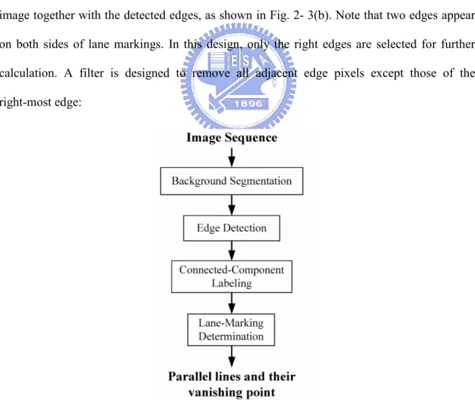
(27) In Chapter 5, we present a design of automatic contour initialization and image tracking of multiple vehicles. Furthermore, a method is proposed to automatically estimate the turn ratio at an intersection by using techniques of detection window as well as optical flow calculation. Chapter 6 shows the experiment of traffic parameter estimation. Finally, conclusions and recommendations for further research are provided in Chapter 7.. Fig. 1-1. Structure of the thesis.. 13.

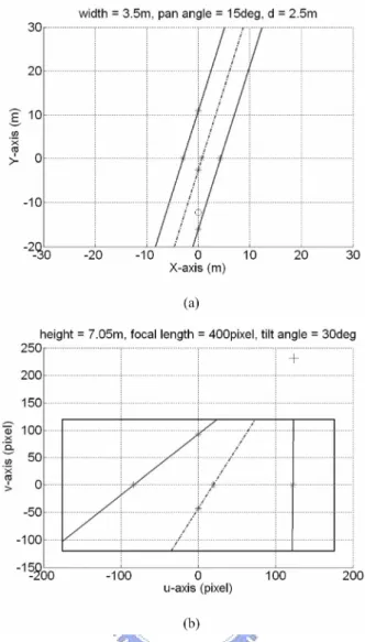
(28) Chapter 2 Dynamic Camera Calibration 2.1 Introduction Current camera calibration techniques for traffic monitoring use more than one set of parallel lines and other known information, such as the tilt and height of the camera, to obtain the camera parameters [20]-[22]. It is easy to select or prepare enough sets of parallel lines for camera calibration in general applications. However, there is frequently only one set of parallel lines on a road. To obtain the camera parameters with reduced known information, it is necessary to generate a second line perpendicular to the existing lines for extracting the camera parameters in a traffic scene. Wang used a set of parallel lanes and a special line perpendicular to the lanes to calibrate the camera [15]. The drawback is that it is impractical to establish an unnecessary line on a road. Schoepflin and Dailey employed the bottom edges of vehicles to obtain the other sets of parallel lines for camera calibration [23]. However, the trajectories of moving vehicles degrade the extracted parallel lines. In this chapter, we present a method that uses a set of parallel lines in combination with the known height of the installed camera to calibrate the camera. The rest of this chapter is organized as follows. Section 2.2 presents the derivation of camera calibration equations for the focal length, the pan angle, as well as the tilt angle. Section 2.3 describes image processing algorithms for lane-marking detection. Synthetic sensitivity analysis and experimental results of camera parameter estimation are presented in Section 2.4. Section 2.5 summarizes the contribution of this design. The detailed derivation of 14.

(29) focal length equation is presented in Appendix A. Appendix B describes the conversion between pixel coordinates and world coordinates.. 2.2 Focal Length Equation The objective of camera calibration is to determine all the required parameters for estimating the world coordinates from the pixel coordinates (u, v) of a given point in an image frame. In the following presentation, it is assumed that the change of camera height and intrinsic parameters, except for the focal length, are negligible as the camera view changes. These parameters can be considered as fixed in image-based traffic applications and calibrated only once during PTZ camera installation. A method for computing the changeable camera parameters, including the focal length, the pan and tilt angles, will be presented below. Fig. 2-1 illustrates three coordinate systems utilized in the derivation: the world coordinate system (X, Y, Z), the camera coordinate system (Xc, Yc, Zc), and the camera-shift coordinate system (U, V, W). Fig. 2-1(a) depicts the top view of the ground plane in the world coordinate system, lines L1, L2 and L3 represent parallel lane markings, and point O is the. Fig. 2-1. Coordinate systems used in the PTZ camera calibration. (a) Top view of road map on world coordinate system. (b) Side view of camera setup and its coordinate systems used in calibration. (c) Road schematics used in the pixel-based coordinate system.. 15.

(30) origin of the world coordinate system on the road plane. The pan angle θ is defined by the angle between Y-axis and lane markings, f is the focal length, and w is the width between parallel lanes. The symbol d denotes a shift distance, which is a perpendicular distance between the projection of the principle point of camera and L3. Fig. 2-1(b) depicts the side view of the road scene, which is used to describe the geometric relationship between the ground plane and the camera; the direction of vector CO is perpendicular to the image plane. In Fig. 2-1(b), φ is the tilt angle of the camera, h is the installed camera height, and F is the length of vector CO . In this chapter, the counterclockwise rotation is positive in expressing the sign of angles. The camera-shift coordinate system can be obtained by rotating the world coordinate system at an angle φ around the X-axis. The relationship between the camera-shift coordinate frame and the world coordinate frame is given by: 0 U  1  V  = 0 cos φ    W  0 sin φ. 0  X  − sin φ   Y  . cos φ   Z . (2.1). By shifting the camera-shift coordinate frame from point O to point C along the vector OC and inversing the V-axis of the camera shift coordinate frame, one can obtain the camera coordinate system. The camera coordinates of any point on the road plane (where Z equals to 0) can be expressed as a function of world coordinates via a coordinate transformation between the camera-shift coordinate frame and the world coordinate frame: 0   X c   U  1 0  Y  =  W  = 0 sin φ   X  −  0  .  c    Y     Z c  − V − F  0 − cos φ     F . (2.2). As given by the pin-hole camera model [22], any point in camera coordinates has a perspective projection on the image plane. The relationship between pixel coordinates and camera coordinates can be written as: 16.

(31) u =−f. Xc X , =−f Zc − Y cos φ − F. v=−f. Yc Y sin φ . =−f Zc − Y cos φ − F. (2.3). (2.4). The pixel coordinate system is shown in Fig. 2-1(c); the rectangular region represents the sensing area of the image sensor. Solid lines represent the lane markings that can be observed by the camera. Dashed lines denote the lane markings that are out of the field of view of the camera and cannot be observed. The parallel lines in Fig. 2-1(a) are projected onto a set of lines in Fig. 2-1(c) that intersect at a point known as vanishing point (VP). The vanishing point lies at a position where Y coordinate of (X, Y, Z) approaches infinite. The coordinate (u 0 , v0 ) of VP is given by u0 = lim u = lim (− f Y − >∞. Y − >∞. X Y tan θ ) = f tan θ sec φ , ) = lim (− f Y − >∞ − Y cos φ − F − Y cos φ − F. v0 = lim v = lim (− f Y − >∞. Y − >∞. Y sin φ ) = f tan φ . − Y cos φ − F. (2.5). (2.6). In this study, we propose to use parallel lane markings to establish a geometric relationship between a road plane and its camera view. As shown in Fig. 2-1(a), L1, L2 and L3 intersect X-axis and Y-axis at six points; these points are denoted by P1–P6, respectively. From the perspective model, the corresponding coordinates of these points in image plane can be obtained. Through geometric analysis, deriving the focal length equation expressed below is a straightforward process: am 2 + bm + c = 0 ,. where m is f. 2. (2.7). and Table 2-1 summarizes the variables used in (2.7). The detailed. derivation is presented in Appendix A.. 17.

(32) Table 2-1 List of Variables for Focal Length Equation. The solution f 2 of (2.7) must be positive. Accordingly, the focal length f is f = m.. (2.8). Using (2.6), the tilt angle is given by. φ = tan −1. v0 . f. (2.9). From (2.5), the pan angle is expressed as. θ = tan −1. u0 f sec φ .. (2.10). If (2.7) has two positive roots, then the meaningful solution will be the one that satisfies (A.24). Using the camera parameters, one can transform the pixel coordinates into their corresponding world coordinates (X,Y,0) [63], the detailed procedure is described in Appendix B. 18.

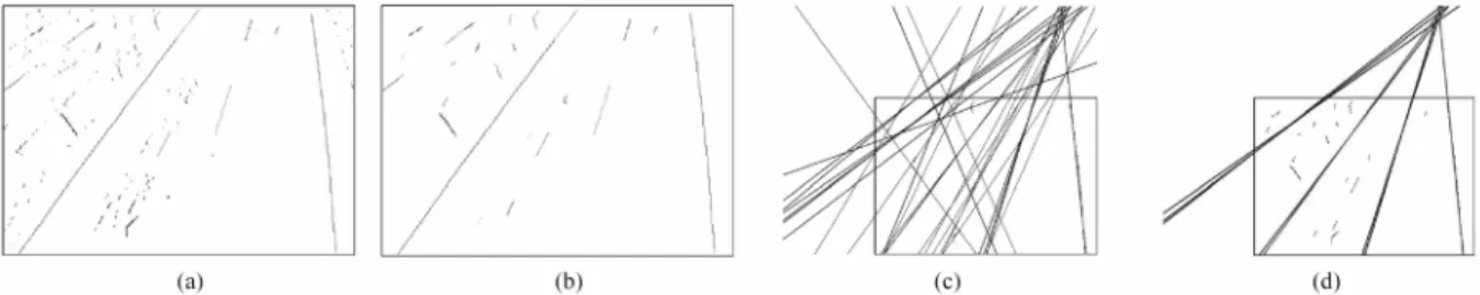
(33) 2.3 Detection of Parallel lane Markings In this section, an image processing procedure is proposed to automatically detect parallel lane markings in road imagery. The complete procedure consists of background segmentation, edge extraction, erosion, dilation, labeling, and lane marking analysis. Fig. 2-2 shows the functional block diagram of the image processing procedure.. 2.3.1 Edge Detection From the extracted background image, the edges of lane markings can be obtained adopting an intensity gradient method [64]. The detected edges of traffic lane markings are depicted in Fig. 2- 3(a). To verify the detection performance, we examine the background image together with the detected edges, as shown in Fig. 2- 3(b). Note that two edges appear on both sides of lane markings. In this design, only the right edges are selected for further calculation. A filter is designed to remove all adjacent edge pixels except those of the right-most edge:. Fig. 2-2. System architecture of image-based lane-marking determination.. 19.

(34) P (u , v) = 0 if. u +5. ∑ P ( j , v) ≥ 1 ,. (2.11). j = u +1. where P(u , v) is the binary value at (u, v) in the edge map. Fig. 2-3(c) depicts the filtered result. The left edges of lane markings are removed as expected. An erosion operation is then employed to remove salt-and-pepper noise and shrink the detected edge [64]. Next, a dilation operation is applied to reconnect discontinuous features, which belong to a same object [65]. Fig. 2-3(d) shows the final result of edge detection. It is clear that the salt-and- pepper noise is removed and the extracted edges are ready for lane-marking analysis.. 2.3.2 Connected-Component Labeling and Lane-Marking Determination As depicted in Fig. 2-3(d), lane-marking segments are longer than the features generated by other object such as trees, bushes, guideposts, etc. Using a connected-component labeling operation [66], one can classify and label the pixels that are linked together. Fig. 2-4(a) shows the labeling result of the binary image of Fig. 2-3(d). The count (length) of connected pixels can be used to determine whether the connected pixels are features of a lane marking or not. Only those with larger count are preserved; the rest will be removed. The result of this operation is illustrated in Fig. 2-4(b). On a multi-lane road, the lane markings of the road edges are normally indicated by solid lines, while the lane divider lines are marked by broken lines. Based on this premise, labeled segments that have the first and the second largest number are considered as the sides of a multi-lane road. They are termed as sidelines. Each. Fig. 2-3. Edge maps of background image. (a) Edge map. (b) Background image and its associated edge map. (c) Right-side edge map. (d) Denoised edge map.. 20.

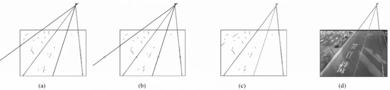
(35) sideline will then be represented by a linear polynomial equation: y = λx + ρ ,. (2.12). where λ and ρ are real numbers. One can use a least-square approximation to obtain λ and ρ . Accordingly, the intersection of sidelines can be computed. It gives us the vanishing point of parallel lane markings. Other segments are similarly processed to obtain their first-degree polynomial equations, as plotted in Fig. 2-4(c). Next, these lines are checked whether they parallel the sidelines in the real world. If a straight line is parallel with the sidelines, then the intersection of the line with the sidelines needs to be located within a vanishing-point region ( Vr ): Vr = {(u , v) : (u − u 0 ) 2 + (v − v0 ) 2 ≤ 13} ,. (2.13). where (u 0 , v 0 ) is the vanishing point. Most lines, which are not parallel with the sidelines, will be removed by this intersection discrimination. As shown in Fig. 2-4(d), only those lines satisfying (2.13) are reserved. In order to correctly locate all the lane markings on the road, the disconnected segments, which belong to a broken lane-divider line, must be merged into a line for obtaining a correct least-square linear representation. A criterion has been developed to find those lines which are near to each other. Fig. 2-5(a) shows the result after merging such lines in of Fig. 2-4(d). As. Fig. 2-4. Linear approximation of lane markings. (a) Labeled feature map. (b) Labeled segment with larger count are kept. (c) Linear approximations map. (d) The lines which intersect the sidelines and locate within a vanishing-point region are reserved.. 21.

(36) shown in Fig. 2-5(a), although with reduced line numbers, extra lines still might exist in the image. Only the lane-divider lines that lie inside the sidelines need to be kept; others must be removed as well. Exploiting the assumption that each traffic lane is of the same width on the road, one can apply a virtual horizontal line to intersect each candidate line to obtain its position information in the image plane. As shown in Fig. 2-5(b), circles are used to represent the positions of the candidate lines and star symbols are used to represent the position of sidelines that have already been found. As shown in Fig. 2-5(b), the line with a circle lies in the center of two stars will be the lane-divider line. Fig. 2-5(c) shows the detected lane markings and their vanishing point. Fig. 2-5(d) illustrates the background image together with the detected lane markings. This lane-marking detection algorithm is computationally efficient compared with popular Hough transform approaches. A video clip of the image processing. steps. for. finding. parallel. lane. markings. can. be. found. at. http://isci.cn.nctu.edu.tw/video/JCTai/Lane_detection.mpg.. 2.4 Experimental Results To demonstrate the performance of the proposed calibration algorithm, we first use synthetic traffic data to carry out a sensitivity analysis and then validate the calibration results using actual traffic images.. Fig. 2-5. Parallel-lane markings and their vanishing point. (a) Parallel-line map. (b) Location map of parallel lines. (c) Parallel-lane markings map. (d) Background image and its associated parallel-lane markings. 22.

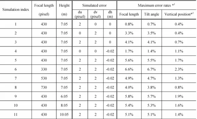
(37) 2.4.1 Sensitivity Analysis In actual applications, there might be intrinsic or extrinsic errors of camera calibration that cause measurement error. For example, the principle point might vary with zooming [10], making pixel coordinates incorrect. Radial distortion also affects the accuracy of parallel lane detection. Tilt or pan operations will change the height of the image sensor and cause errors in the focal length estimation. In order to assure the robustness of the proposed calibration method, we present a sensitivity analysis on the focal length estimation using synthetic data containing intrinsic and extrinsic errors. Fig. 2-6(a) illustrates the synthetic traffic scene with two parallel lanes.. The circle in. the figure represents the camera. The camera view of Fig. 2-6(a) is constructed according to (2.3) and (2.4); the result is shown in the rectangle region of Fig. 2-6(b). Three lines of image view intersect one another at the vanishing point, which is denoted by a cross in Fig. 2-6(b). The camera parameters–such as tilt angle, pan angle, and focal length–are calculated from the synthetic data using the calibration method described in Section 2.2. In the simulation, the tilt angle is changed from 30 to 60 degrees and the pan angle is changed from -20 to 20 degrees. These angles reflect most situations in actual ITMS applications. To emulate the effect caused by radial distortion or incorrect principle-point position, the vanishing point is shifted two pixels upward, to the right, and diagonally. New parallel lines are established in accordance with the new vanishing point and the intersections of the original lines and the u-axis. Using (2.7), focal length is calculated in accordance with these new parallel lines. In the simulation, the height of the camera is set to 7.05m and the focal length is set to 430 pixels. The maximum error rates calculated for the condition of translational error in, respectively, horizontal, vertical, and diagonal directions are presented in simulations 1, 2, and 3 of Table 2-2. The absolute error rates of focal length estimation are within 4.1%. Furthermore, the result reveals that the focal length estimation is more sensitive to vertical than horizontal 23.

(38) translational error. It is observed from the sensitivity analysis that the tilt angle estimation is also more sensitive to vertical translational error. The absolute error rates of the tilt angle are within 4.1%. Because the estimated parameters will be employed to estimate the position of vehicle in ITMS, the error rates of the position in the image frame are calculated accordingly. The absolute error rates of vertical position are within 0.7% at pixel coordinate (150, 120). To investigate the effect of inaccurate camera height, we introduced a height error of -0.02m into the simulation. Traffic view is generated according to the true height (7.05m); the focal length is then estimated using the inaccurate height data. Simulation 4 of Table 2-2 shows Table 2-2 Maximum Error Rates of Focal Length, Tilt Angle and Vertical Position under Different Simulated Error. 24.

(39) Fig. 2-6. Synthetic traffic scene for simulation. (a) Top view of a road scene. (b) The road view in image plane.. that three kinds of error rates are all within 1.7%. Detailed error-rate results are presented in Fig. 2-7 to examine estimation of focal length, tilt angle, and position, respectively. It is observed that for a tilt angle less than 30 degrees or an absolute pan angle greater than 20 degrees, the error rates will become unacceptable. This phenomenon is mainly caused by the fact that in the image plane the parallel lanes and their vanishing point will deviate more seriously due to radial distortion and incorrect principle-point position. In addition, diagonal error and height error are also simulated. The error rates are all within 5.6%, as shown in simulation 5 of Table 2-2.. 25.

(40) Fig. 2-7. Sensitivity analysis of translation and height errors.. greater than 20 degrees, the error rates will become unacceptable. This phenomenon is mainly caused by the fact that in the image plane the parallel lanes and their vanishing point will deviate more seriously due to radial distortion and incorrect principle-point position. In. 26.

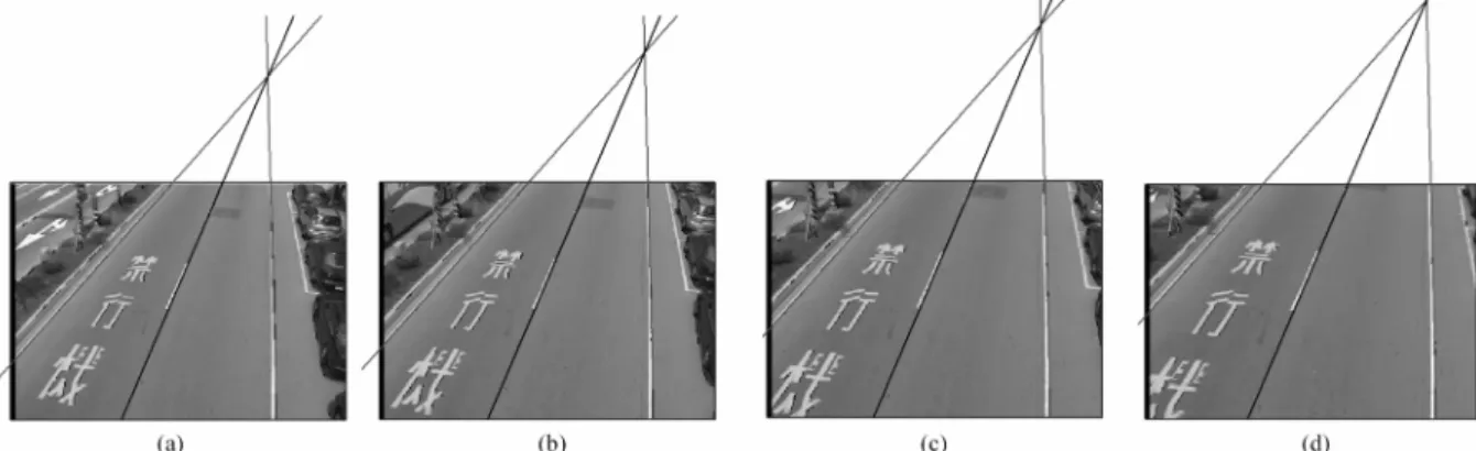
(41) addition, diagonal error and height error are also simulated. The error rates are all within 5.6%, as shown in simulation 5 of Table 2-2. As for the case of translational error and height error, simulations 6, 7, and 8 of Table 2-2 show the simulation results with a focal length of 330, 530, and 730 pixels, respectively. The absolute error rates of focal length and tilt angle are within 6.7% and the absolute error rates of vertical translational position are within 2.3%. The results reveal that the larger the focal length, the less the error rate. Finally, for cases with translational error and height error, simulations 9, 10, and 11 of Table 2-2 show the simulation results of a height of 6.05m, 8.05m, and 10.05m, respectively. The absolute error rates of the focal length and the tilt angle are within 5.8%. The absolute error rates of the vertical position are within 2%. The results reveal that the higher the camera, the less the error rates. Furthermore, the effect of height change is not obvious in the test. From the synthetic analysis, the errors introduced by extrinsic and intrinsic errors are within 6.7% (focal length = 330 pixels). These error rates of position measurement are acceptable for traffic monitoring.. 2.4.2 Experiments with Actual Imagery The proposed algorithm has been tested with image sequences recorded from a main road near National Chiao Tung University. The camera used in the experiments is a SONY EVI-D31 digital camera. The image sequences were captured with a resolution of 352*240 pixels. For traffic monitoring, the camera was installed at a height of 7.03m and the width between parallel lane markings is 3.52m. In the experiments, the background image was first segmented and then used for the lane-marking detection. The vanishing point and the camera parameters–such as the focal length, tile angle, and pan angle–were calculated using (2.7), (2.9), and (2.10), respectively. To validate the estimated parameters, twelve sample features were assigned in a traffic scene for distance measurement, as shown in Fig. 2-8. To 27.

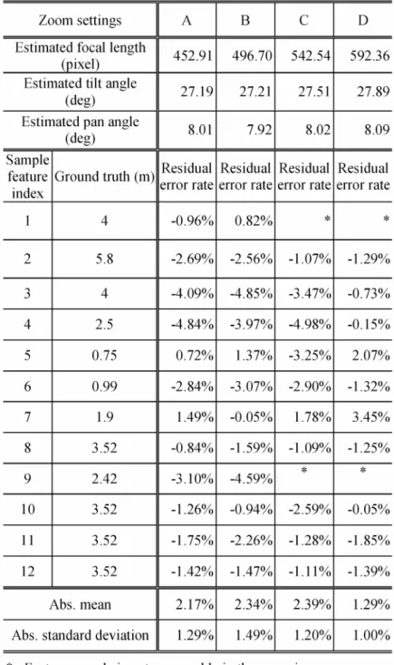
(42) Fig. 2-8. Sample features selected for image measurement in road imagery.. Fig. 2-9. Traffic images captured under different zoom settings. (a) Image of zoom setting A. (b) Image of zoom setting B. (c) Image of zoom setting C. (d) Image of zoom setting D.. validate the estimated parameters, twelve sample features were measured manually and compared with the estimated distances for evaluation. The estimated distances were computed based on the calibrated camera parameters. In the first experiment, traffic images with different zoom settings (A, B, C and D) were captured to demonstrate the robustness to the radial distortion, as shown in Fig. 2-9. The principle point of the camera is practically fixed for these zoom settings. The experiment results are listed in Table 2-3. The focal lengths are estimated to be 452.91, 496.70, 542.54, and 592.36 pixels, respectively, for the four different zoom settings. Using the focal length, angle are 27.45 and 0.33 degree, respectively. The estimated mean and standard deviation of 28.

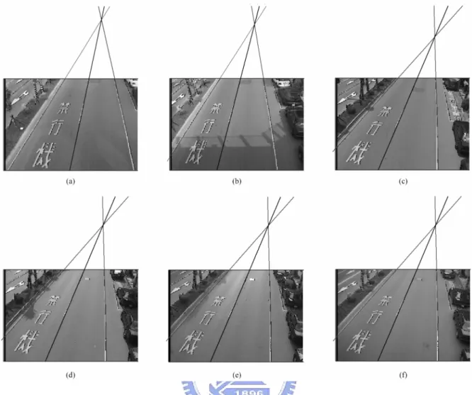
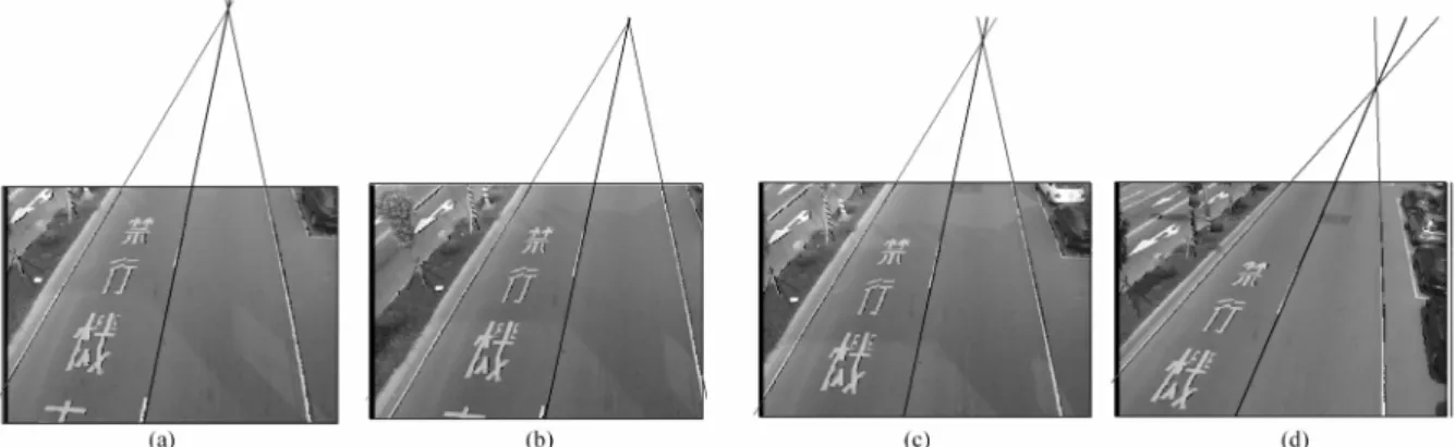
(43) Table 2-3 Calibration Results under Different Zoom Settings. the pan angle are 8.01 and 0.07 degree. These experimental results show that error rates of absolute mean and standard deviation are within 2.39% and 1.49%. The proposed calibration algorithm gives satisfactory accuracy and is robust against zoom changes. To evaluate the robustness of lane detection with respect to variation in environmental illumination, we took images at various hours of a sunny day. Six sets of image sequences are presented to show different illumination conditions, as shown in Fig. 2-10. The intensity 29.

(44) Fig. 2-10. Traffic images captured under different illumination conditions. (a) Image with weak shadow. (b) Image with strong shadow. (c) Image under bright illumination. (d) Image under soft illumination. (e) Image captured at sunset. (f) Image under darker illumination.. values of lane markings vary in these image frames, but the lane markings always have higher intensities than their adjacent region. The gradient can be successfully used to detect the edge of lane markings, as discussed in Section 2.3. The results reveal that the lane detection method performs satisfactorily under different lighting conditions. This robustness partly results from the fact that the SONY PTZ camera has auto exposure and backlight compensation functions to ensure that the subject remains bright even in harsh backlight conditions. Finally, the algorithm is evaluated with a fixed zoom under different pose settings (A, B, C and D) of the PTZ camera, as shown in Fig. 2-11. Table 2-4 shows the experimental results of the estimation of feature sizes as depicted in Fig. 2-8. The mean and standard deviation of 30.

(45) Fig. 2-11. Traffic images captured under different camera pose settings. (a) Image of pose setting A. (b) Image of pose setting B. (c) Image of pose setting C. (d) Image of pose setting D.. estimated focal lengths are 417.08 and 9.56 pixels, respectively. The mean and the standard deviation of absolute error rates among these measurements are within 2.32% and 1.58%. The experimental results of different zoom and view settings show that the maximum calibration error of distance measurement is within 5%, which is comparable to the results achieved by [20] and [21]. However, our method offers improved autonomy and efficiency. A video clip of image processing sequence for traffic parameter estimation can be found at http://isci.cn.nctu.edu.tw/video/JCTai/Speed_detection.mpg.. 2.5 Summary `A novel algorithm has been proposed for automatic calibration of a PTZ camera overlooking a traffic scene. The proposed approach requires no manual operation to select positions of special features. It automatically uses a set of parallel lane markings and the lane width to compute the camera parameters, namely, focal length, tilt angle, and pan angle. Image processing procedures have been developed for automatically finding parallel lane markings. Subsequently, the pan and tilt angles of the camera can be obtained by using the estimated focal length. To locate the parallel lane markings, an image processing procedure has been developed. Synthetic data and actual traffic imagery have been employed to validate accuracy and robustness of the propose method.. 31.

(46) Table 2-4 Calibration Results under Different Camera Pose Settings. 32.