Controlling chaos by GA-based reinforcement learning neural network

Controlling Chaos by GA-Based Reinforcement

Learning Neural Network

Chin-Teng Lin,

Member, IEEE,

and Chong-Ping Jou

Abstract—This paper proposes a TD (temporal difference) and

GA (genetic algorithm) based reinforcement (TDGAR) neural learning scheme for controlling chaotic dynamical systems based on the technique of small perturbations. The TDGAR learning scheme is a new hybrid GA, which integrates the TD prediction method and the GA to fulfill the reinforcement learning task. Structurely, the TDGAR learning system is composed of two integrated feedforward networks. One neural network acts as a critic network for helping the learning of the other network, the action network, which determines the outputs (actions) of the TDGAR learning system. Using the TD prediction method, the critic network can predict the external reinforcement signal and provide a more informative internal reinforcement signal to the action network. The action network uses the GA to adapt itself according to the internal reinforcement signal. This can usually accelerate the GA learning since an external reinforcement signal may only be available at a time long after a sequence of actions have occurred in the reinforcement learning problems. By defin-ing a simple external reinforcement signal, the TDGAR learndefin-ing system can learn to produce a series of small perturbations to convert chaotic oscillations of a chaotic system into desired regular ones with a periodic behavior. The proposed method is an adaptive search for the optimum control technique. Computer simulations on controlling two chaotic systems, i.e., the H´enon map and the logistic map, have been conducted to illustrate the performance of the proposed method.

Index Terms—Chaos, genetic algorithm, periodic control,

rein-forcement learning, temporal difference prediction.

I. INTRODUCTION

C

HAOS is apparently an irregular motion, which is non-linear but deterministic. It tracks a trajectory that is quite complex but not entirely random. Chaos has been observed in many physical systems, such as chemical reactors, fluid flow systems, forced oscillators, feedback control devices, and laser systems [1]. In designing such a system, it is often desired that chaos can be avoided, i.e., certain portion of the parameter space where the system behaves chaotically can be ignored. However, some portion of the parameter space can be significant; neglecting it may be highly undesirable when chaos is useful in some situations. For example, increased drag in flow system, erratic fibrillations of heart beating and complicated circuit oscillations are some situations where

Manuscript received March 12, 1998; revised August 31, 1998 and February 16, 1999. This work was supported by the R.O.C. National Science Council under Grant NSC87-2213-E-009-146.

The authors are with the Department of Electrical and Control Engineering, National Chiao-Tung University, Hsinchu, Taiwan, R.O.C.

Publisher Item Identifier S 1045-9227(99)05485-5.

chaos is harmful. On the contrary, in secure communications chaotic signal can be added to an information signal then transmitted in a secure way. That is, information signal to be transmitted is masked by the noise like chaotic signal by adding it at the transmitter then at the receiver the masking is removed, the information signal cannot be deciphered in general at the receiving end unless full information about the chaotic system is available. One may wish then to design a physical, biological, chemical experiment, or to project an industrial plant to behave in a chaotic manner to achieve a desired performance. Thus, the problem of controlling chaos has been lately begun receiving attention. Researches on the control of chaos in a host of physical systems ranging from lasers and electronic circuits to chemical and biological systems can be reviewed from [8] and references therein.

Controlling chaos is to convert chaotic oscillations into desired regular ones with a periodic behavior. The possibility of purposeful selection and stabilization of particular orbits in a normal chaotic system using minimal predetermined efforts provides a unique opportunity to maximize the output of a dynamical system. It is thus of great importance to develop suitable control methods and to analyze their efficacy. Re-cently, much interest has been focused on this type of problems [2]–[8]. Different control algorithms are essentially based on the fact that one would like to effect changes as minimal as possible to the original system so that it is not grossly deformed. From this point of view, controlling methods or algorithms can be broadly classified into two categories: feedback and nonfeedback methods [9]. Feedback control methods essentially make use of the intrinsic properties of chaotic systems, including their sensitivity to initial conditions, to stabilize orbits already existing in the systems. In contrast to feedback control techniques, nonfeedback methods make use of a small perturbing external force such as a small driving force, a small noise term, a small constant bias, or a weak modulation to some system parameter. All these methods modify the underlying chaotic dynamical system weakly so that stable solutions appear.

In 1990, Ott et al. [2] first proposed a new method (col-loquially called the OGY method) of controlling a chaotic dynamical system by stablizing one of the many unstable periodic orbits embedded in a chaotic attractor, through only small time dependent perturbations in some accessible system parameter. OGY’s method is one kind of feedback control algorithms and has attracted the attention of many physicists interested in applications of nonlinear dynamics. Experimental control of chaos was achieved by Ditto et al. [3] soon after. 1045–9227/99$10.00  1999 IEEE

They applied OGY’s method to control the chaotic vibrations of a magnetoelastic ribbon to achieve stable period-1 and period-2 orbits in the chaotic regime. However, OGY’s method requires monitoring the system long enough to determine a linearization of its behavior in the neighborhood of the desired unstable periodic orbit before it can be applied. Besides, the determination of small nudges of the perturbation requires a knowledge of the eigenvalues and eigenvectors of the unstable orbits. More recently, Alsing et al. [10] used a feedforward backpropagation neural network to stabilize the unstable periodic orbits embedded in a chaotic system. Their controlling algorithm used for training the network is based on OGY’s method, and thus inherits the deficiencies of the OGY’s method mentioned above. Another approach to controlling chaos with a neural network was proposed by Otawara and Fan [11], where the same network structure as Alsing’s was used. Their method approximates the system’s governing equations through judicious perturbation of an accessible parameter of the system. Specifically, it feeds back automatically the deviation of the predicted value at the succeeding iteration from the unstable fixed point on a return map to the parameter. The above two neural-network approaches are both super-vised learning methods, in which a feedforward multilayer neural network is trained by data pairs generated from a chaotic system to produce a time series of small perturbations necessary for control. The disadvantage is that the fixed points of the chaotic system need to be determined and/or the system’s nonlinear dynamics need to be analyzed in advance. However, since the application of neural controllers to chaotic systems has gained great benefits, we therefore expect to give a systematic approach to designing a neural controller for controlling chaos by reinforcement learning method. In this paper, we shall propose a genetic algorithm (GA)-based reinforcement learning scheme to the problems of controlling chaos. This scheme need not know the fixed points of a chaotic system, and can effectively control the system on a high periodic orbit without supervised training data.

In the neural learning methods, supervised learning is effi-cient when the input–output training pairs are available [12]. However, many control problems require selecting control actions whose consequences emerge over uncertain periods for which input–output training data are not readily available. In such a case, the reinforcement learning method can be used to learn the unknown desired outputs by providing the system with a suitable evaluation of its performance. Two general approaches are for reinforcement learning; the

actor-critic architecture and the GA. The former approach uses the

temporal difference (TD) method to train a critic network that learns to predict failure. The prediction is then used to heuristically generate plausible target outputs at each time step, thereby allowing the learning of the action network that maps state variables to output actions [12]–[15]. The action and critic networks can be neuron-like adaptive elements [13], multilayer neural networks [17], or neural fuzzy networks [18], [19]. The main drawback of these actor critic architectures is that they usually suffer the local minima problem in network learning due to the use of gradient descent (ascent) learning method.

GA’s are general purpose optimization algorithms with a probabilistic component that provides a means to search poorly understood irregular spaces [21]. From the network learning point of view, since GA’s only need the suitable evaluation of the network performance to yield the fitness values for evolution, they are suitable for the reinforcement learning problems [22]–[25]. As compared to the aforementioned ac-tor critic architecture, all the above GA-based reinforcement learning schemes use only the action networks. Without the predictions (internal critics) of the critic network, the GA cannot proceed to the new generation until the arrival of the external reinforcement signals. This causes the main drawback of these pure GA approaches, i.e., very slow convergence, since an external reinforcement signal may only be available at a time long after a sequence of actions has occurred in the reinforcement learning problems.

In this paper, we integrate the actor critic architecture and GA into a new reinforcement learning scheme. This scheme can solve the local minima problem in the actor-critic architecture by making use of the global optimization capability of GA’s. Also, it can efficiently speed up the convergence of GA’s with the prediction capability of the actor critic architecture. The proposed scheme is called the TD and GA-based reinforcement (TDGAR) learning method. Structurely, the TDGAR learning system is constructed by integrating two feedforward multilayer networks. One neural network acts as the critic network for helping the learning of the action network, and the other neural network acts as the action network for determining the outputs (actions) of the TDGAR learning system. Using the TD prediction method, the critic network can predict the external reinforcement signal and provide a more informative internal reinforcement signal to the action network. The action network uses the GA to adapt itself according to the internal reinforcement signal. The key concept of the proposed TDGAR learning scheme is to formulate the internal reinforcement signal as the fitness function of the GA such that the GA can evaluate the candidate solutions (chromosomes) regularly even during the period without external reinforcement feedback from the environ-ment. Hence, the GA can proceed to new generations regularly without waiting for the arrival of the external reinforcement signal. The proposed TDGAR learning method is applied to the controlling chaos problems in this paper based on the technique of small perturbations. By defining a simple external reinforcement signal, the TDGAR learning system can learn to produce a series of small perturbations to convert chaotic oscillations of a chaotic system into desired regular ones with a periodic behavior. Computer simulations on controlling two chaotic systems, i.e., the H´enon map and the logistic map, will be conducted to illustrate the performance of the proposed method.

This paper is organized as follows. Section II describes the concept of using small perturbations to control chaos. Section III describes the basic of GA’s. The structure of the proposed TDGAR learning system and the corresponding learning algorithm are presented in Section IV. In Section V, the TDGAR learning method is applied to control two chaotic systems. Finally, conclusions are summarized in Section VI.

II. USINGSMALL PERTURBATIONS TOCONTROL CHAOS The presence of chaos may be of a great advantage for control in a variety of situations. In a practical situation involving a real physical apparatus, one may expect that chaos is avoided or that the system dynamics is changed in some way so that improved performance can be obtained. Given a chaotic attractor, one might consider making some large, possibly costly, change in the system to achieve the desired objective. In a nonchaotic system, small control signals typically can only change the system dynamics slightly. Short of applying large control signals or greatly modifying the system, it is stuck with whatever system performance already exists. However, in a chaotic system it is free to choose among a rich variety of dynamical behaviors. Thus, it may be advantageous to design chaos into systems, allowing such variety without requiring large control signals or the design of separate systems for each desired behavior.

Ott et al. [2] prescribed a method to transform a system initially in a chaotic state into a controlled periodic one. There exits an infinite number of unstable periodic orbits embedded in the attractor, and only small, carefully chosen perturbations are necessary to stabilize one of these. That is, one can select a desired behavior from the infinite variety of behaviors naturally present in chaotic systems, and then stabilize this behavior by applying only tiny changes to an accessible system parameter [8]. Lima and Pettini [26] have suggested that it is possible to bring a chaotic system into a regular regime by means of a small parametric perturbation of suitable frequency. In addition, the effect of an additional weak constant bias term to quench chaos has also been reported in [27]. All these methods are based on the idea of using small changes to perturb a chaotic system. Let us consider a return or iterated map

(1) where is the accessible parameter of the system that can be externally perturbed, is the state value at the th iteration, and is the state value at the ( )th iteration. Inspired by the above mentioned methods, giving a small change to the system parameter, we can express the perturbed map as the following form:

(2) where is the time-varying small change to alter system parameter. Another form of small perturbations is

(3) where the function of is just like an external force acting on the chaotic system to quench chaos. Our goal is to design a neural controller to find this small perturbation signal such that chaos can be controlled.

Chaotic systems exhibit extremely sensitive dependence on initial conditions, i.e., two identical chaotic systems starting at nearly the same point follow orbits that divert rapidly from each other and become quickly uncorrelated. For example, if we run a chaotic system two times starting at the same initial conditions; one is computed with single precision and

the other with double precision, then one chaotic orbit will closely approach the other chaotic orbit in the first few iterations, but will then rapidly move far apart. Those orbits in chaotic systems are unstable in the sense that small deviation from the periodic orbit grows exponentially rapidly in time, and the system orbit quickly moves away from the periodic orbit. Occasionally, the chaotic orbit may closely approach a particular unstable periodic orbit, in which case the chaotic orbit would approximately follow the periodic cycle for a few periods, but it would then rapidly move away because of the instability of the periodic orbit. Therefore, adding a small perturbation on a chaotic system will cause a large variation on the orbit except that the orbit is closely around the fixed points. Hence, when the chaotic state is in the neighborhood of the fixed point, only a small perturbation applied to a system parameter will let it fall into the vicinity of the fixed point in the next iteration; otherwise, even when the state is exactly on a fixed point with no small perturbation to stabilize it, it will move apart from the fixed point eventually.

Neural networks are attractive for use as controllers of complex systems, because they do not require the models of the dynamical systems to be controlled. A neural network with inputs being fed by a time series of values of the phase space variables of a chaotic system can be trained to produce a time series of proper small perturbations for controlling chaos. In this paper, we shall use reinforcement learning scheme to learn the unknown desired outputs (perturbations) by providing the learning system with a suitable function (reinforcement signal) for evaluating its performance. Usually, it is difficult to define a reinforcement signal for controlling a chaotic system, because no apparent information is revealed to indicate whether a control action is good or bad. However, inspired by the idea mentioned in the above paragraph, (i.e., when a chaotic state is closely around the fixed point, a small perturbation will stabilize it on the fixed point), we can define the reinforcement signal by a limitation on the magnitudes of perturbations, i.e., a predefined maximum perturbation is used as a constraint. When the perturbation is within the predefined maximum perturbation range, the reinforcement signal will indicate the control action being a successful trial; otherwise, it is a failure trial. One big advantage of this learning control scheme is that we need not know the fixed point of the controlled chaotic system in advance because a series of successful trials (meaning that a series of proper small perturbations are allowed to apply to the system) has indicated that the system states are around a fixed point. Thus, the magnitude of the small perturbation provides a good indicator of the target point.

For the control of higher period orbits, we further propose a scheme called periodic control. In this scheme, unlike the control of a period-1 orbit, where the chaotic system is perturbed by a small perturbation in each iteration, we perturb the chaotic system every N iterations for the control of a period- orbit. The periodic control learns to find any one of the points on the period- orbit depending on the position of the initial states, and view it as a fixed point for control. In other words, the periodic control reduces the period-control problem to a period-1 period-control problem. In this way,

the controller is switched on to keep the system stay in one of the period- points every iterations, and then switched off to let the system run freely to reach other period- points by making use of the periodic feature of the period- chaotic orbit. Hence, in our proposed TDGAR learning system, it is free to select the target for the control of a period- orbit. However, in the learning process of periodic control, it is possible that the control of a period- orbit falls into any one of the period- , period- , or period-1 points. Hence, we have to check the learned stabilized point to see if it is the same as any one of the following -1 points in the next -1 free running iterations. If so, the stabilized point is not a period- point and we have to restart the learning with new initial states. In the next section, we give a brief description of the genetic algorithm and in Section IV we shall describe the proposed learning system deliberately.

III. GENETIC ALGORITHMS

GA’s are invented to mimic some of the processes observed in natural evolution. The underlying principles of GA’s were first published by Holland [20]. The mathematical framework was developed in the 1960’s and was presented in Holland’s pioneering book [21]. GA’s have been used primarily in two major areas: optimization and machine learning. In optimiza-tion applicaoptimiza-tions, GA’s have been used in many diverse fields such as function optimization, image processing, the traveling salesman problem, system identification, and control. In ma-chine learning, GA’s have been used to learn syntactically simple string IF–THEN rules in an arbitrary environment. Excellent references on GA’s and their implementations and applications can be found in [28] and [30].

The GA is a general purpose stochastic optimization method for search problems. GA’s differ from normal optimization and search procedures in several ways. First, the algorithm works with a population of strings, searching many peaks in parallel. By employing genetic operators, it exchanges information between the peaks, hence lowering the possibility of ending at a local minimum and missing the global minimum. Second, it works with a coding of the parameters, not the parameters themselves. Third, the algorithm only needs to evaluate the objective function to guide its search, and there is no require-ment for derivatives or other auxiliary knowledge. The only available feedback from the system is the value of the per-formance measure (fitness) of the current population. Finally, the transition rules are probabilistic rather than deterministic. The randomized search is guided by the fitness value of each string and how it compares to others. Using the operators on the chromosomes which are taken from the population, the algorithm efficiently explores parts of the search space where the probability of finding improved performance is high.

The basic element processed by a GA is the string formed by concatenating substrings, each of which is a binary coding of a parameter of the search space. Thus, each string represents a point in the search space and hence a possible solution to the problem. Each string is decoded by an evaluator to obtain its objective function value. This function value, which should be maximized or minimized by the GA, is then converted to a

fitness value which determines the probability of the individual undergoing genetic operators. The population then evolves from generation to generation through the application of the genetic operators. The total number of strings included in a population is kept unchanged through generations. A GA in its simplest form uses three operators: reproduction, crossover, and mutation [28]. Through reproduction, strings with high fitnesses receive multiple copies in the next generation while strings with low fitnesses receive fewer copies or even none at all. The crossover operator produces two offspring (new candidate solutions) by recombining the information from two parents in two steps. First, a given number of crossing sites are selected along the parent strings uniformly at random. Second, two new strings are formed by exchanging alternate pairs of selection between the selected sites. In the simplest form, crossover with single crossing site refers to taking a string, splitting it into two parts at a randomly generated crossover point and recombining it with another string which has also been split at the same crossover point. This procedure serves to promote change in the best strings which could give them even higher fitnesses. Mutation is the random alteration of a bit in the string which assists in keeping diversity in the population. Roughly speaking, GA’s manipulate strings of binary digits, “1’s” and “0’s,” called chromosomes which represent multiple points in the search space through proper encoding mechanism. Each bit in a string is called an allele. GA’s carry out simulated evolution on populations of such chromosomes. Like nature, GA’s solve the problem of finding good chromosomes by manipulating the material in the chromosomes blindly without any knowledge about the type of problem they are solving. The only information they are given is an evaluation of each chromosome they produce. The evaluation is used to bias the selection of chromosomes so that those with the best evaluations tend to reproduce more often than those with bad evaluations. GA’s, using simple manipulations of chromo-some, such as simple encodings and reproduction mechanisms, can display complicated behavior and solve some extremely difficult problems without knowledge of the decoded world.

The encoding mechanisms and the fitness function form the links between the GA and the specific problem to be solved. The technique for encoding solutions may vary from problem to problem and from GA to GA. Generally, encoding is carried out using bit strings. The coding that has been shown to be the optimal one is binary coding [21]. Intuitively, it is better to have few possible options for many bits than to have many options for few bits. A fitness function takes a chromosome as input and return a number or a list of numbers that is a measure of the chromosome’s performance on the problem to be solved. Fitness functions play the same role in GA’s as the environment plays in natural evolution. The interaction of an individual with its environment provides a measure of fitness. Similarly, the interaction of a chromosome with a fitness function provides a measure of fitness that the GA uses when carrying out reproduction.

In this paper, we develop a novel hybrid GA called the TD and GA-based reinforcement learning method, which integrates the TD prediction method and the GA into the actor critic architecture to fulfill the reinforcement learning task.

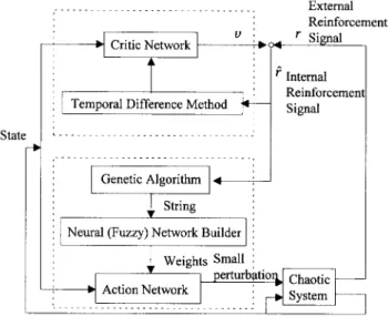
Fig. 1. The proposed TDGAR learning system for controlling chaos.

IV. TD- AND GA-BASED REINFORCEMENT LEARNING SYSTEM

The proposed TDGAR learning method is a kind of hybrid GA algorithms [28]. Traditional simple GA’s, though robust, are generally not the most successful optimization algorithm on any particular domain. Hybridizing a GA with algorithms currently in use can produce an algorithm better than the GA and the current algorithms [30]–[33] GA’s may be crossed with various problem specific search techniques to form a hybrid that exploits the global perspective of the GA (global

search and the convergence of the problem-specific technique

(local search). In some situations, hybridization entails using the representation as well as optimization techniques already in use in the domain, while tailoring the GA operators to the new representation. In this connection, the proposed TDGAR learning method is a hybrid of GA and the actor critic archi-tecture which is a quite mature technique in the reinforcement learning domain. The TDGAR method is an adaptive search for the optimum control technique. We shall next introduce the structure and learning algorithm of the TDGAR learning system in the following sections.

A. Structure of the TDGAR Learning System

The proposed TDGAR learning system is constructed by integrating two feedforward multilayer networks. One neural network acts as a critic network for helping the learning of the other network, the action network, which determines the outputs (actions) of the TDGAR learning system as shown in Fig. 1. Both the critic network and the action network have exactly the same structure as that shown in Fig. 2. The TDGAR learning system is basically in the form of the actor critic architecture [14]. Since we want to solve the reinforcement learning problems in which the external reinforcement signal is available only after a long sequence of actions have been passed onto the environment plant, we need a multistep critic network to predict the external reinforcement signal. In the TDGAR learning system, the critic network models the environment such that it can perform

Fig. 2. The structure of the critic network and the action network in the TDGAR learning system.

a multistep prediction of the external reinforcement signal that will eventually be obtained from the environment for the current action chosen by the action network. With the multistep prediction, the critic network can provide a more informative internal reinforcement signal to the action network. The action network can then determine a better action to impose onto the environment in the next time step according to the current environment state and the internal reinforcement signal. The internal reinforcement signal from the critic network enables both the action network and the critic network to learn at each time step without waiting for the arrival of an external reinforcement signal, greatly accelerating the learning of both networks. The structures and functions of the critic network and the action network are described in the following sections.

1) The Critic Network: The critic network constantly

pre-dicts the reinforcement associated with different input states, and thus equivalently, evaluates the goodness of the control actions determined by the action network. The only infor-mation received by the critic network is the state of the environment in terms of state variables and whether or not a failure has occurred. The critic network is a standard two layer feedforward network with sigmoids in the hidden layer and output layer. The input to the critic network is the state of the plant, and the output is an evaluation of the state, denoted by . This value is suitably discounted and combined with the external failure signal to produce the internal reinforcement signal, .

Fig. 2 shows the structure of the critic network. It includes hidden nodes and input nodes including a bias node (i.e., ). In this network, each hidden node receives inputs and has weights, while each output node receives inputs and has weights. The output of each hidden node is given by

(4)

where

and are successive time steps, and is the weight from the th input node to the th hidden node. The output node of the critic network receives inputs from the hidden nodes (i.e.,

) and directly from the input nodes (i.e., )

(6)

where is the prediction of the external reinforcement value, is the weight from the th input node to the output node, and is the weight from the th hidden node to the output node. Unlike the supervised learning problem in which the correct “target” output values are given for each input pattern to instruct the network learning, the reinforcement learning prob-lem has only very simple “evaluative” or “critic” information available for learning rather than “instructive” information. In the extreme case, there is only a single bit of information to indicate whether the output is right or wrong. The environment supplies a time-varying input vector to the network, receives its time varying output/action vector and then provides a time varying scalar reinforcement signal. In this paper, the external

reinforcement signal is two-valued, ,

such that means “a success” and

means “a failure.” We also assume that is the external reinforcement signal available at time step and is caused by the inputs and actions chosen at earlier time steps, (i.e., at time steps ). To achieve the control goal by the proposed TDGAR learning system, we have to define a proper external reinforcement signal. According to the key concept of controlling chaos by using small perturbations discussed in Section II, we define the external reinforcement signal as

if

otherwise (7)

where is a predefined maximum perturbation value. From the analysis in Section II, we understand that the action network will produce large perturbations to repress chaotic oscillations when the state of the chaotic system falls out-side the controlling region, (i.e., the period-1 orbit). On the other side, when the state of the chaotic system falls in the controlling region, the action network only needs to produce small perturbations to maintain the regular state trajectory of the chaotic system. Hence, the magnitude of the perturbation produced by the action network is a good indicator to see the performance of the TDGAR learning system. According to (7), the learning system will get an external reinforcement signal with value zero indicating “success” when the produced perturbation is small enough; otherwise, it will get a signal with value one indicating “failure.”

The critic network evaluates the action recommended by the action network and represents the evaluated result as the internal reinforcement signal. The internal reinforcement signal is a function of the external failure signal and the change

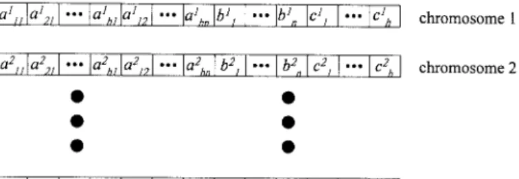
Fig. 3. The encoding of the neural network in Fig. 2 on chromosomes.

in state evaluation based on the state of the system at time start state failure state otherwise

(8) where is the discount rate. In other words, the change in the value of plus the value of the exter-nal reinforcement sigexter-nal constitutes the heuristic or interexter-nal reinforcement signal, , where the future values of are discounted more the further they are from the current state of the system.

2) The Action Network: The action network is to determine

a proper action acting on the environment (plant) according to the current environment state. In our TDGAR learning system, the structure of the action network is exactly the same as that of the critic network shown in Fig. 2. The only information received by the action network is the state of the environment in terms of state variables and the internal reinforcement signal from the critic network. In applying GA’s for neural-network learning, the connection weights of the action network are encoded as genes (or chromosomes), and GA’s are then used to search for better solutions (optimal structures and parameters) for the action network. Fig. 3 shows the encoding of the action network on chromosomes with population size . Bit string encoding is the most common encoding technique used by GA researchers because of its ease of creating and manipulating. However, binary string encoding usually causes longer search time than the real-valued string encoding. Hence, connection weights of the action network are encoded here as a real-valued string. Initially, the GA generates a population of real-valued strings randomly. An action network corresponding to each string then runs in a feedforward fashion to produce control actions acting on the environment according to (4) and (6). At the same time, the critic network constantly predicts the reinforcement associated with changing environment states under the control of the current action network. After a fixed time period, the internal reinforcement signal from the critic network will indicate the “fitness” of the current action network. This evaluation process continues for each string (action network) in the population. When each string in the population has been evaluated and given a fitness value, the GA can look for a better set of strings and apply genetic operators on them to form a new population as the next generation. Better actions can thus be chosen by the action network in the next generation.

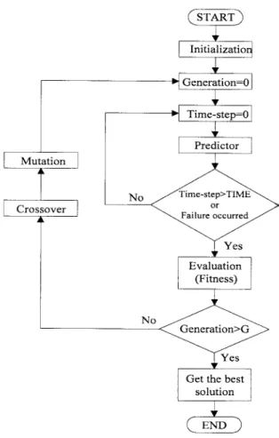
Fig. 4. The flowchart of the proposed TDGAR learning method.

After a fixed number of generations, or when the desired control performance is achieved, the whole evolution process is stop, and the string with the largest fitness value in the last generation is selected and decoded into the final action network. The detailed learning scheme for the action network will be discussed in the next section.

B. Learning Algorithm of the TDGAR Learning System

The flowchart of the TDGAR learning algorithm is shown in Fig. 4. In the following sections, we first consider the reinforcement learning scheme for the critic network of the TDGAR system, and then introduce the GA-based reinforce-ment learning scheme for the action network of the TDGAR system.

1) Learning Algorithm for the Critic Network: When both

the reinforcement signal and input patterns from the envi-ronment depend arbitrarily on the past history of the action network outputs and the action network only receives a rein-forcement signal after a long sequence of outputs, the credit assignment problem becomes severe. This temporal credit

assignment problem results because we need to assign credit or

blame to each step individually in long sequences leading up to eventual successes or failures. Thus, to handle this class of reinforcement learning problems, we need to solve the temporal credit assignment problem along with solving the original structural credit assignment problem concerning attri-bution of network errors to different connections or weights.

The solution to the temporal credit assignment problem in the TDGAR system is to use a multistep critic network that predicts the reinforcement signal at each time step in the period without any external reinforcement signal from the environment. This can ensure that both the critic network and the action network can update their parameters during the period without any evaluative feedback from the environment. To train the multistep critic network, we use a technique based on the temporal difference method, which is often closely related with the dynamic programming techniques [13], [34], [35]. Unlike the single step prediction and the supervised learning methods which assign credit according to the difference between the predicted and actual outputs, the temporal difference methods assign credit according to the difference between temporally successive predictions. Note that the term “multistep prediction” used here means the critic network can predict a value that will be available several time steps later, although it does such prediction at each time step to improve its prediction accuracy.

The goal of training the multistep critic network is to minimize the prediction error, i.e., to minimize the internal reinforcement signal, . It is similar to a reward/punishment scheme for the weights updating in the critic network. If pos-itive (negative) internal reinforcement is observed, the values of the weights are rewarded (punished) by being changed in the direction which increases (decreases) its contribution to the total sum. The weights on the links connecting the nodes in the input layer directly to the nodes in the output layer are updated according to the following rule:

(9) where is the learning rate and is the internal reinforcement signal at time .

Similarly, for the weights on the links between the hidden layer and the output layer, we have the following weight update rule:

(10) The weight update rule for the hidden layer is based on a modified version of the error backpropagation algorithm [36]. Since no direct error measurement is possible (i.e., knowledge of correct action is not available), plays the role of an error measure in the update of the output node weights; if is positive, the weights are altered so as to increase the output for positive input, and vice versa. Therefore, the equation for updating the hidden weights is

(11) Note that the sign of a hidden node’s output weight is used, rather than its value. The variation is based on Anderson’s empirical study [17] that the algorithm is more robust if the sign of the weight is used rather than its value.

2) Learning Algorithm for the Action Network: The GA is

used to train the action network by using the internal reinforce-ment signal from the critic network as the fitness function.

Initially, the GA randomly generates a population of real-valued strings, each of which represents one set of parameters for the action network. The real value encoding scheme instead of the normal binary encoding scheme in GA’s is used here, so recombination can only occur between weights. A population of small size is used in our learning scheme. This reduces the exploration of the multiple (representationally dissimilar) solutions for the same network.

After a new real-valued string is created, an interpreter takes this real-valued string and uses it to set the parameters in the action network. The action network then runs in a feedforward fashion to control the environment (plant) for a fixed time period (determined by the constant “ ” in Fig. 4) or until a failure occurs. At the same time, the critic network predicts the external reinforcement signal from the controlled environment and provides an internal reinforcement signal to indicate the “fitness” of the action network. In this way, according to a defined fitness function, a fitness value is assigned to each string in the population, where high fitness values mean good fit. The fitness function, , can be any nonlinear, nondifferentiable, discontinuous, positive function, because the GA only needs a fitness value assigned to each string. In this paper, we use the internal reinforcement signal from the critic network to define the fitness function

(12) which reflects the fact that small internal reinforcement values, (i.e., small prediction errors of the critic network) mean higher fitness of the action network, where is the current time step, , and the constant “ ” is a fixed time period during which the performance of the action network is evaluated by the critic network. If an action network receives a failure signal from the environment before the time limit, (i.e., ), then the action network that can keep the desired control goal longer before failure occurs will obtain higher fitness value. The above fitness function is different from that defined normally in the pure GA approach [24], where the relative measure of fitness takes the form of an accumulator that determines how long the experiment is still “success.” Hence, a string (action network) cannot be assigned a fitness value until an external reinforcement signal arrives to indicate the final success or failure of the current action network.

When each string in the population has been evaluated and given a fitness value, the GA then looks for a better set of strings to form a new population as the next generation by using genetic operators, (i.e., the reproduction, crossover, and mutation operators). In basic GA operators, the crossover operation can be generalized to multipoint crossover in which the number of crossover points is defined. With set to one, generalized crossover reduces to simple crossover. The multipoint crossover can solve one major problem of the simple crossover; one point crossover cannot combine certain combinations of features encoded on chromosomes. In the proposed GA-based reinforcement learning algorithm, we choose . The crossover operation for real value encoding is demonstrated in Fig. 5. For the mutation operator,

(a)

(b)

Fig. 5. Illustration of crossover operation for real-value strings. (a) before crosssover. (b) After crosssover.

(a)

(b)

Fig. 6. Illustration of mutation operation for real-value string. (a) Before mutation. (b) After mutation.

since we use the real value encoding scheme, we use a higher mutation probability in our algorithm. This is different from the traditional GA’s that use the binary encoding scheme. The latter are largely driven by recombination, not mutation. The operation of mutation is done by adding a randomly selected value within the range 10 to a randomly selected site of the chromosome. Fig. 6 shows an example illustrating the mutation operation. The above learning process continues to new generations until the number of generations meets a predetermined stop criterion. After the whole evolution process is stop, the string with the largest fitness value in the last generation is selected and decoded into the final action network.

The major feature of the proposed hybrid GA learning scheme is that we formulate the internal reinforcement signal as the fitness function for the GA based on the actor-critic architecture. In this way, the GA can evaluate the candidate solutions (the weights of the action network) regularly during the period without external reinforcement feedback from the environment. The GA can thus proceed to new generations in fixed time steps (specified by the constant “ ”) without waiting for the arrival of the external reinforcement signal. In other words, we can keep the time steps ( ) for evalu-ating each string (action network) and the generation size ( )

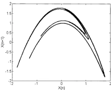
Fig. 7. The H´enon attractor.

fixed in our learning algorithm (see the flowchart in Fig. 3), since the critic network can give predicted reward/penalty information to a string without waiting for the final success or failure. This can usually accelerate the GA learning since an external reinforcement signal may only be available at a time long after a sequence of actions has occurred in the reinforcement learning problems. This is similar to the fact that we usually evaluate a person according to his/her potential or performance during a period, not after he/she has done something really good or bad.

V. SIMULATIONS AND RESULTS

In this section, we apply the proposed TDGAR learning method to control two chaotic systems, H´enon map and logistic map. These maps have been extensively studied for decades as examples of producing chaos from a simple algebraic expression. We shall demonstrate the power of the TDGAR learning method by controlling these two chaotic systems on period-1, period-2, or period-4 orbits without analysis of the system’s nonlinear dynamics.

A. Controlling of H´enon Map

H´enon map is a two dimensional mapping with the corre-lation dimension approximately equal to 1.25 given by

(13) This mapping becomes chaotic oscillations when the param-eters in (13) are set as and [10]. In this case, the chaotic state trajectory of this system is shown in Fig. 7, which is obtained by iterating (13) for 10 times. To control the H´enon map by the small perturbation technique discussed in Section II [see (2) or (3)], a small perturbation,

, is added to (13)

(14) The perturbation, , is generated by the action network of the TDGAR learning system (see Fig. 1), and acts on the

H´enon map at each iteration. The control goal is to stabilize the H´enon map on its unstable period-1 orbit, (i.e., fixed point).

There are two input state variables to the TDGAR learning system: , the state variable of the H´enon map at the th iteration; , the state variable at the th iteration. The used critic network and action network in the TDGAR learning system are three-layer neural networks shown in Fig. 2, both with three input nodes, five hidden nodes, and one output node. Hence, there are 23 weights in each network. A bias node fixed at 0.5 is used as the third input to the network, a weight from the bias node to a hidden node (or to the output node) in effect changes the threshold behavior of that node. We use the fitness function defined in (12),

i.e., , in the TDGAR learning system,

where is the internal reinforcement signal from the critic network, which is to predict the external reinforcement signal in (7). The learning parameters used in the TDGAR system are the maximum perturbation , the population sizes , the learning rate , the discount rate , the time limit , and the generation sizes is not limited here. Initially, we set all the weights in the critic network and action network as random values between 2.5 and 2.5.

The TDGAR learning process proceeds as follows. We first randomly generate 200 (population size) chromosomes corresponding to 200 initial action networks. For each action network, there is a critic network with random initial weights associated with it to form a TDGAR learning system as shown in Fig. 1. These 200 TDGAR learning systems are trained and evaluated one by one as follows. In the beginning, the initial state values of the controlled chaotic system are fed into the critic network and the action network. The action network then work in a feedforward fashion to produce perturbation for controlling the chaotic system, and the critic network produces a output value, , to predict the exter-nal reinforcement sigexter-nal. The produced perturbation is then evaluated and an external reinforcement signal is generated according to (7). With this external reinforcement signal, the critic network will tune itself to get better prediction in the future. The new state values of the chaotic system are then sent back to the inputs of the action and critic networks, and starts the next iteration. After 100 (time limit) iterations, the critic network will produce an internal reinforcement signal according to (8) to give the action network a final and detailed evaluation. However, it should be noted that at the beginning of learning (30 time steps used here), larger perturbations are allowed such that the action network can find more feasible solutions for the perturbations so as to force the state of the H´enon map fall into the controlling region quickly from any initial point. After 30 time steps, we begin to check if the perturbations are within a predefined maximum perturbation range. With the internal reinforcement signal available, a fitness value can be obtained by (12). In this way, when each of the 200 action networks has been evaluated and given a fitness value, the GA then looks for a better set of action networks to form a new population by using genetic operators and starts the next generation.

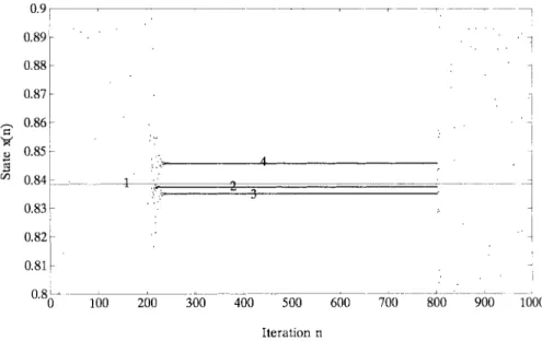
Fig. 8. Control of the H´enon map on the period-1 orbit by using different predefined maximum perturbation values as learning criteria.

Fig. 9. Control of the H´enon map on the period-1 orbit by the TDGAR learning system.

The details of the learning process has been described in Section IV-B. Repeat the above, learning process regularly from generation to generation. A control strategy (i.e., an action network) was deemed successful if it could stabilize the H´enon map on its period-1 orbit, i.e., the fixed point of the H´enon map.

In the following tests, we define different allowed maximum perturbation values, , to see the learning efficiency of the TDGAR learning system. Three maximum perturbation

values are defined as , ,

and for learning criteria [see (7)]. After learning, three corresponding action networks (controllers) are obtained to stabilize the H´enon map successfully. In the test, the controller is switched on, [i.e., the small perturbations produced by the action network are added to the H´enon map as in (14)] at iteration , and is switched off at iteration

. The results are shown in Fig. 8, where orbit “1” denotes the period-1 orbit (fixed point) of the H´enon map, orbit “2” is the stabilized orbit when the controller is trained under the criteria , orbit “3” is the stabilized orbit when the controller is trained under the criteria , and orbit “4” is the stabilized orbit when the controller is trained under the criteria . It is observed that the H´enon map stays around its fixed point, , stably during the control process. Once the control signal is removed, the system evolves chaotically. Moreover, it is observed that more strictly the maximum perturbation value is allowed, more closely the H´enon map is stabilized to its fixed point. However, higher accuracy is achieved at the cost of lower learning speed.

Fig. 9 shows the results of controlling the H´enon map by the learned TDGAR controller under the criteria

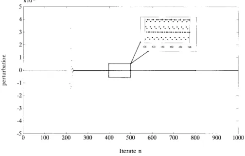
Fig. 10. Control signal from the action network of TDGAR in controlling the H´enon map on the period-1 orbit.

Fig. 11. The logistic map.

. We see that the H´enon map stays on its period-1 orbit stably during the control process. An enlargement of the square in Fig. 9 shows the precise state values of the controlled chaotic system from iteration to iteration . Corresponding to Fig. 9, Fig. 10 shows the control signals (perturbations) produced by the action network of the learned TDGAR system. It shows that only a few larger perturbations are needed to repress chaotic oscillations at the beginning of the control process, and then quite small perturbations are enough to keep the H´enon map stay on its period-1 orbit. An enlargement of the square in Fig. 10 also shows the precise control signals (perturbations) during the control process from

iteration to iteration . The enlargement

pictures in Figs. 9 and 10 show that the small perturbation, , presented in (14) [also refer to (3)] is not just a static shift of operation points (constant); it is more like a dynamical external force acting on the chaotic system to quench chaos from time to time.

B. Controlling of Logistic Map

In this simulation, we apply the TDGAR learning system to control what is considered the simplest, but one of the most interesting dynamical system, the logistic map

(15) This map is often used to model population dynamics. The parameter is the nonlinearity parameter; when the mapping is chaotic [11]. The fixed point for the period-1 orbit is . The fixed points for the period-2 orbit are

and . The logistic map is

an one dimensional map. Fig. 11 shows the state trajectory of the logistic map with obtained by iterating (15) for times. When adding small perturbations to control the logistic map, the perturbed logistic map has the form of [see (2)]

(16) or [see (3)]

(17) In the TDGAR learning system for controlling the logistic map, the fitness function and the external reinforcement signal are defined to be the same as those used before, i.e., (7) and (12). Since there is only one input state variable in this case, the used critic network and action network both have two input nodes (including the bias node), four hidden nodes and one output node. The learning parameters used are the same as those in the previous example. The initial state is randomly selected between zero and one so as to get nontrivial dynamical behavior.

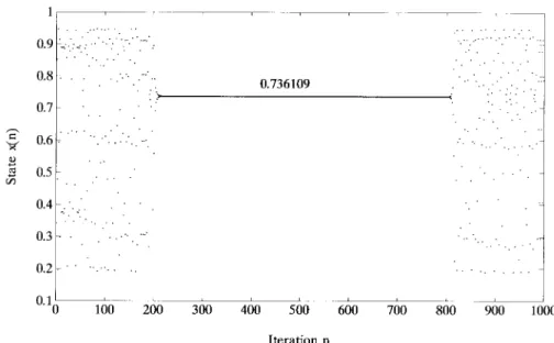
Fig. 12 shows the results of controlling the logistic map on the period-1 orbit. It shows that the orbit of the controlled logistic map remains around the fixed point

Fig. 12. Control of the logistic map on the period-1 orbit by the TDGAR learning system.

Fig. 13. Control of the logistic map on the period-2 orbit by the TDGAR learning system.

as long as the controller is switched on. As for the control of period-2 orbits, we propose a scheme called periodic control. We observe on the period-2 orbit of the logistic map that when is closely in the proximity of , it will automatically triggered to the next fixed point , and then bounds back to . This happens periodically. Hence, the periodic control scheme adds a small perturbation to the chaotic system only at every other iteration of the system. Consequently, the external reinforcement signal is also available at every other iteration in the learning process. In other words, the controller is switched on to keep the system stay in one fixed point at one iteration, and then switched off to let the system run freely to reach another fixed point at the next iteration. In this way, the controller is switched on and off periodically. Fig. 13 shows the results of controlling the logistic map on a period-2 orbit, where the orbit is highly stabilized during the control process.

Apparently, the initial state determines which period-2 point to be stabilized by the controller. For example, if the initial state is close to the period-2 point , it is more likely that the controller will learn to control this point rather than the other period-2 point . In the simulations, we did observe this situation. When we set the initial state as , the final learned controlled point was . When we set the initial state as , the final learned controlled

point was . As mentioned at the end of

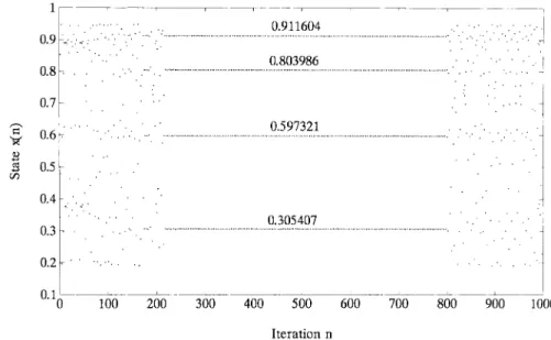
Section II, it was possible that the period-2 control failed and fell into period-1 control, when the initial state was very close to the period-1 orbit (fixed point) . When this happened, we assigned new initial state and restarted the learning process. The idea of periodic control can be easily extended to the control of higher periodic orbits. Fig. 14 shows the results of controlling the logistic map on a period-4 orbit,

Fig. 14. Control of the logistic map on the period-4 orbit by the TDGAR learning system.

where the controller is switched on every four iterations of the logistic map. Note that the orbit is highly stabilized during the control process. The TDGAR learning system also shows a good efficiency of control on a high periodic orbits. However, our simulations show that higher order orbits are more difficult, (i.e., take longer learning time) to stabilize than the lower order ones (as they are in the OGY’s method), partially because of the false learning of the period- /2, period- /4, points. In our simulations, the learning for controlling the logistic map on period-1 orbit took 2235 generations, on period-2 orbit took 29 341 generations, and on period-4 orbit took 208 363 generations.

In the above simulations, we used the deterministic maps, i.e., the H´enon map and the logistic map, as test examples. This was done purely for numerical convenience, and also because these two maps have been widely used as benchmarks for the researches of controlling chaos. Since the TDGAR learning system need not know the mathematical model or the property (such as fixed points) of the controlled chaotic system, it is immaterial to the TDGAR learning system whether the chaotic signals are generated analytically or experimentally from real world. In other words, the above simulations demonstrate the feasibility of applying the proposed TDGAR learning system for controlling chaos in a practical situation involving a real physical apparatus. We therefore expect our system to be applicable to some realistic objects as diverse as synchronized chaotic oscillators [37], magnetoelastic ribbon system [3], nonlinear electrical oscillator [9], and chaotic laser system [38]. Because of the success of controlling chaos by the proposed TDGAR learning system, we are now working on the research of synchronization of chaos, especially for secure communication.

It is noted that although the H´enon map and logistic map have generally wide nonchaotic parameter regions in which a return map will show a similar result as what being controlled in the above simulations, our purpose is to develop a systematic approach to designing a neural controller against

chaotic system by reinforcement learning method. In other words, we are interested in stablizing the chaotic parameter region of a chaotic system, instead of looking for its nonchaotic parameter region in this research.

VI. CONCLUSION

This paper integrates the TD technique, gradient descent method, and GA into the actor-critic architecture to form a new reinforcement learning system, called the TDGAR learning system. By the TDGAR learning system, we can train a neural controller for the plant according to a simple reinforcement signal. The proposed TDGAR learning method makes the design of neural controllers more feasible and practical for real world applications, since it greatly lessens the quality and quantity requirements of the teaching signals, and reduces the long training time of a pure GA approach. The TDGAR learning system has been successfully applied to control two simulated chaotic systems by incorporating the techniques of small perturbations and periodic control in this paper. The simulation results showed that the TDGAR learning system can learn to produce a series of small perturbations to convert chaotic oscillations of a chaotic system into desired regular ones with a periodic behavior including period-1, period-2, and period-4 orbits. Since the TDGAR learning system need not know the mathematical model or the property (such as fixed points) of the chaotic system for control, it can be applied to control a physical chaotic system in the real-world directly.

REFERENCES

[1] F. C. Moon, Chaotic and Fractal Dynamics. New York: Wiley, 1992, pp. 1–46.

[2] E. Ott, C. Grebogi, and J. A. Yorke, “Controlling chaos,” Phys. Rev.

Lett., vol. 64, pp. 1196–1199, 1990.

[3] W. D. Ditto, S. N. Rauseo, and M. L. Spano, “Experimental control of chaos,” Phys. Rev. Lett., vol. 65, pp. 3211–3214, 1990.

[4] J. Singer, Y. Z. Wang, and H. H. Bau, “Controlling a chaotic system,”

Phys. Rev. Lett., vol. 66, pp. 1123–1125, 1991.

[5] A. Garfinkl, M. L. Spano, W. L. Ditto, and J. N. Weiss, “Controlling cardiac chaos,” Science, vol. 257, pp. 1230–1235, 1992.

[6] U. Dressler and G. Nitsche, “Controlling chaos using time delay coordinates,” Phys. Rev. Lett., vol. 68, pp. 1–4, 1992.

[7] F. J. Romeiras, C. Grebogi, E. Ott, and W. P. Dayawansa, “Controlling chaotic dynamical system,” Phys. D, vol. 58, pp. 165–192, 1992. [8] T. Shinbrot, E. Ott, C. Grebogi, and J. A. Yorke, “Using small

pertur-bations to control chaos,” Nature, vol. 363, pp. 411–417, 1993. [9] M. Lakshmanan and K. Murali, Chaos in Nonlinear Oscillators:

Con-trolling and Synchronization. Singapore: World, 1996.

[10] P. M. Alsing, A. Gavrielides, and V. Kovanis, “Using neural networks for controlling chaos,” Phys. Rev. E., vol. 49, pp. 1225–1231, 1994. [11] K. Otawara and L. T. Fan, “Controlling chaos with an artificial neural

networks,” in Proc. IEEE Int. Joint Conf. Fuzzy Syst., 1995, vol. 4, pp. 1943–1948.

[12] A. G. Barto and M. I. Jordan, “Gradient following without backpropa-gation in layered network,” in Proc. Int. Joint Conf. Neural Networks, San Diego, CA, 1987, vol. II, pp. 629–636.

[13] A. G. Barto, R. S. Sutton, and C. W. Anderson, “Neuronlike adaptive elements that can solve difficult learning control problem,” IEEE Trans.

Syst., Man, Cybern., vol. SMC-13, pp. 834–847, 1983.

[14] R. S. Sutton, “Temporal credit assignment in reinforcement learning,” Ph.D. dissertation, Univ. Massachusetts, Amherst, 1984.

[15] A. G. Barto and P. Anandan, “Pattern recognizing stochastic learning automata,” IEEE Trans. Syst. Man Cybern., vol. SMC-15, pp. 360–375, 1985.

[16] R. J. Williams, “A class of gradient estimating algorithms for rein-forcement learning in neural networks,” in Proc. Int. Joint Conf. Neural

Networks, San Diego, CA, 1987, vol. II, pp. 601–608.

[17] C. W. Anderson, “Strategy learning with multilayer connectionist repre-sentations,” in Proc. 4th Int. Workshop Mach. Learn., Irvine, CA, June 1987, pp. 103–114.

[18] H. R. Berenji and P. Khedkar, “Learning and tuning fuzzy logic controllers through reinforcements,” IEEE Trans. Neural Networks, vol. 3, pp. 724–740, 1992.

[19] C. T. Lin and C. S. G. Lee, “Reinforcement structure/parameter learning for an integrated fuzzy neural network,” IEEE Trans. Fuzzy Syst., vol. 2, pp. 46–63, Feb. 1994.

[20] J. H. Holland, “Outline for a logical theory of adaptive systems,” J.

Assoc. Comput. Machinery, vol. 3, pp. 297–314, 1962.

[21] , Adaptation in Natural and Artificial System. Ann Arbor, MI: Univ. Michigan, 1975.

[22] S. Harp, T. Samad, and A. Guha, “Designing application specific neural networks using the genetic algorithm,” Neural Information Processing

Systems, vol. 2. San Mateo, CA: Morgan Kaufmann, 1990. [23] J. D. Schaffer, R. A. Caruana, and L. J. Eshelman, “Using genetic search

to exploit the emergent behavior of neural networks,” Phys. D, vol. 42, pp. 244–248, 1990.

[24] D. Whitley, S. Dominic, R. Das, and C. W. Anderson, “Genetic reinforcement learning for neurocontrol problems,” Machine Learning, vol. 13, pp. 259–284, 1993.

[25] D. E. Moriarty and R. Miikkulainen, “Efficient reinforcement learning through symbiotic evolution,” Machine Learning, vol. 22, pp. 11–32, 1996.

[26] R. Lima and M. Pettini, “Suppression of chaos by resonant parametric perturbations,” Phys. Rev., vol. A41, pp. 726–733, 1990.

[27] K. Murali, M. Lakshmanan, and L. O. Chua, “Controlling and synchro-nization of chaos in the simplest dissipative nonautonomous circuit,”

Int. J. Bifurcation and Chaos Appl. Sci. Eng., vol. 5, pp. 563–571, 1995.

[28] D. E. Goldberg, Genetic Algorithms in Search, Optimization and

Ma-chine Learning. Reading, MA: Addison-Wesley, 1989.

[29] E. L. Lawler, Combinatorial Optimization: Networks and Matroids. New York: Holt, Rinehart and Winston, 1976.

[30] L. Davis, Handbook of Genetic Algorithms. New York: Van Nostrand Reinhold, 1991.

[31] D. Adler, “Genetic algorithms and simulated annealing: A marriage proposal,” in Proc. IEEE Int. Conf. Neural Networks, San Francisco, CA, 1993, vol. II, pp. 1104–1109.

[32] L. Tsinas and B. Dachwald, “A combined neural and genetic learning algorithm,” in Proc. IEEE Int. Conf. Neural Networks, 1994, vol. I, pp. 770–774.

[33] V. Petridis, S. Kazarlis, A. Papaikonomou, and A. Filelis, “A hybrid genetic algorithm for training neural networks,” in Artificial Neural

Networks 2, I. Aleksander and J. Taylor, Eds. Amsterdam, The Nether-lands: North Holland, 1992, pp. 953–956.

[34] R. S. Sutton, “Learning to predict by the methods of temporal differ-ence,” Machine Learning, vol. 3, pp. 9–44, 1988.

[35] P. J. Werbos, “A menu of design for reinforcement learning over time,” in Neural Networks for Control, W. T. Miller, III, R. S. Sutton, and P. J. Werbos, Eds. Cambridge, MA: MIT Press, 1990, ch. 3.

[36] D. Rumelhart, G. Hinto, and R. J. Williams, “Learning internal repre-sentation by error propagation,” in Parallel Distributed Processing, D. Rumelhart and J. McCelland, Eds. Cambridge, MA: MIT Press, 1986, pp. 318–362.

[37] L. M. Pecora and T. L. Carroll, “Synchronization in chaotic systems,”

Phys. Rev. Lett., vol. 64, no. 8, pp. 821–824, 1990.

[38] A. Hohl, A. Gavrielides, T. Erneux, and V. Kovanis, “Localized synchronization in two coupled nonidentical semiconductor laser,” Phys.

Rev. Lett., vol. 78, no. 25, pp. 63–66, 1997.

Chin-Teng Lin (S’88–M’91) , for a photograph and biography, see this issue, p. 845.

Chong-Ping Jou was born in Taiwan, R.O.C., in 1960. He received the B.S. degree in electrical engi-neering from the Chung-Cheng Institute of Technol-ogy, Taiwan, in 1982, the M.S. degree in electrical engineering from the National Taiwan Institute of Technology, in 1988, and now is the Ph.D. candidate in Chiao-Tung University, Hsinchu, Taiwan.

He is currently the Assistant Researcher in the Chung-Shan Institute of Science and Technology, Tao-Yuan, Taiwan. His research interests include neural network, chaos, and fuzzy control.